Use of an Active Learning Strategy Based on Gaussian Process Regression for the Uncertainty Quantification of Electronic Devices ^†

Abstract

This paper presents a preliminary version of an active learning (AL) scheme for the sample selection aimed at the development of a surrogate model for the uncertainty quantification based on the Gaussian process regression. The proposed AL strategy iteratively searches for new candidate points to be included within the training set by trying to minimize the relative posterior standard deviation provided by the Gaussian process regression surrogate. The above scheme has been applied for the construction of a surrogate model for the statistical analysis of the efficiency of a switching buck converter as a function of seven uncertain parameters. The performance of the surrogate model constructed via the proposed active learning method is compared with that provided by an equivalent model built via a Latin hypercube sampling. The results of a Monte Carlo simulation with the computational model are used as reference.

1. Introduction

Uncertainty quantification represents a key resource for the design of complex electronic devices, since it allows quantifying statistically the effects of possible uncertain design parameters (e.g., the components tolerances) on the system’s performance [1].

Monte Carlo (MC) simulation can be seen as the most straightforward way to carry out the above statistical analysis. The underlying idea is to estimate the probability density function (pdf) of the outputs of interest by collecting the results of a large number of deterministic simulations calculated on a random set of configurations of the unknown parameters, drawn according to their probability distributions. Within the plain implementation of the MC method, the deterministic simulations are run with the so-called computational model. Such a deterministic model can be considered as the most accurate synthetic approximation of the system under modeling able of providing, for any configurations of the system parameters, a prediction of the system’s outputs. Despite its accuracy, a plain implementation of the MC method turns out to be computationally heavy, since, in order to guarantee the convergence of the statistical quantities of interest (e.g., means and standard deviation), it requires us to run a large number of simulations (usually in the order of thousands) with the expensive computational model.

Surrogate models, also known as metamodels, can be considered as an effective solution to reduce the computational cost of MC simulations [2,3,4,5,6]. They provide a closed-form and fast-to-evaluate approximation of the non-linear input-output behavior of the computational model, thereby providing an efficient alternative, which can be directly embedded within the MC simulation flow. Surrogate models are constructed via either regression or fitting techniques from a limited set of simulation results, called training samples, computed with the computational model. Several regressions techniques with different features have been successfully adopted in many fields and applications for the construction of surrogate models ranging from least-squares approaches [2] to the more recent kernel and machine learning regressions (e.g., support vector machine [3], least-square support vector machine [4], Gaussian process regression (GPR) [5,6]). However, the use of the most appropriate regression technique does not guarantee good model accuracy, since the latter is also influenced by the training samples used to train it. A common approach is to select the training samples based on a Latin hypercube sampling (LHS) scheme [7], in which the configurations of the input parameters used to train the model are selected in order to cover the experimental space as much as possible.

This work investigates the possible advantages and the performance of an alternative approach for the sampling selection given by the combination of an active learning (AL) scheme and the GPR [8,9,10,11,12]. The effectiveness of the proposed AL technique has been investigated by considering the uncertainty quantification of the DC efficiency of a switching converter as a function of seven uncertain parameters. The performance of the model built with the help of the proposed AL scheme is compared with that of an equivalent model in which the training samples were computed via plain LHS, by using as references the results of a MC simulation with the computational model.

2. Methods

2.1. Gaussian Process Regression (GPR)

The discussion starts introducing the GPR. Under the assumption that a generic non-linear computational model $\mathcal{M}$, which provides a non-linear input-output map $y=\mathcal{M}\left(\mathbf{x}\right)$ between the parameters $\mathbf{x}\in \mathcal{X}\subset {\mathbb{R}}^d$ and output of interest $y\in \mathbb{R}$, follows a Gaussian process (GP) prior, a noise-free GPR reads [13]:

$$\begin{array}{c}\hfill y=\mathcal{M}\left(\mathbf{x}\right)\sim \underset{{\mathcal{M}}_{GPR}\left(\mathbf{x}\right)}{\underbrace{GP(m\left(\mathbf{x}\right),k(\mathbf{x},{\mathbf{x}}^{\prime })}}\end{array}$$

(1)

where ${\mathcal{M}}_{GPR}\left(\mathbf{x}\right)\sim GP(m\left(\mathbf{x}\right),k(\mathbf{x},{\mathbf{x}}^{\prime }))$ is a GP defined by the trend function $m\left(\mathbf{x}\right)$ and covariance function $k(\mathbf{x},{\mathbf{x}}^{\prime })$. A GP extends the concept of a Gaussian distribution from numbers to functions. The trend $m\left(\mathbf{x}\right)$ provides the average function, among the ones drawn from the GP prior, while the covariance provides the correlation between the values of such functions at different point (i.e., $\mathbf{x}$ and ${\mathbf{x}}^{\prime }$) in the parameter space.

The above GP is called prior distribution, since it fixes the properties of the unknown non-linear model, before looking at the training data [13]. In fact, differently from deterministic regressions (e.g., the support vector machine regression and least-square regression), in which the candidate functions of the model are restricted to a specific class of functions (e.g., polynomial, linear, etc.), the GPR model considers as candidate functions for our model ${\mathcal{M}}_{GPR}$ all the possible non-linear functions drawn from the GP prior by letting data “speak” and assigns a probability to each of them [14].

The prior, combined with the information provided by the computational model, allows one to estimate the posterior distribution. Given a set of training samples ${\mathcal{D}}_{1:n}={\left\{({\mathbf{x}}_i,y_i)\right\}}_{i=1}^n$, computed for a given set of configurations of the input parameters ${\mathbf{x}}_i\in \mathcal{X}\subset {\mathbb{R}}^d$, with the computational model $y_i=\mathcal{M}\left({\mathbf{x}}_i\right)$, the posterior distribution approximates the output value $y_{*}=\mathcal{M}\left({\mathbf{x}}_{*}\right)$ for any input $x_{*}$ in terms of a Gaussian distribution, which reads:

$$\begin{array}{c}\hfill p\left(y_{*}\right|{\mathbf{x}}_{*},{\mathcal{D}}_{1:n})\sim N({\mu }_{{\mathbf{x}}_{*}},{\sigma }_{{\mathbf{x}}_{*}}^2),\end{array}$$

(2)

where the posterior mean ${\mu }_{{\mathbf{x}}_{*}}$ and variance ${\sigma }_{{\mathbf{x}}_{*}}^2$ are:

$${\mu }_{{\mathbf{x}}_{*}}=m\left({\mathbf{x}}_{*}\right)+{\mathbf{k}}_{*}{\mathbf{K}}^{-1}\mathbf{y}$$

(3a)

$${\sigma }_{{\mathbf{x}}_{*}}^2=k_{**}-{\mathbf{k}}_{*}{\mathbf{K}}^{-1}{\mathbf{k}}_{*}^T.$$

(3b)

where $\mathbf{y}={[y_1,\dots ,y_L]}^T$, $\mathbf{K}\in {\mathbb{R}}^{L\times L}$ is the correlation matrix in which the entries $K_{ij}=k({\mathbf{x}}_i,{\mathbf{x}}_j)$, ${\mathbf{k}}_{*}=[k({\mathbf{x}}_{*},{\mathbf{x}}_1),\dots ,k({\mathbf{x}}_{*},{\mathbf{x}}_L)]\in {\mathbb{R}}^{1\times L}$ and $k_{**}=k({\mathbf{x}}_{*},{\mathbf{x}}_{*})$.

The above equations require one to specify both the trend and the covariance functions. In this paper, we will consider a GPR built from a GP prior with a constant mean function (i.e., $m\left(\mathbf{x}\right)={\beta }_0$) and a Matern 5/2 covariance function with automatic relevance determination (ARD) hyper-parameters [13]:

$$\begin{array}{c}\hfill k(\mathbf{x},{\mathbf{x}}^{\prime })={\sigma }_f^2\left(1+\sqrt{5}r+\frac{5}{3}{r}^2\right)exp(-\sqrt{5}r),\end{array}$$

(4)

with

$$\begin{array}{c}\hfill r=\sqrt{\sum _{m=1}^d\frac{{(x_m-x_m^{\prime })}^2}{{\sigma }_m^2}},\end{array}$$

(5)

where ${\sigma }_f$ and ${\sigma }_m$ for $m=1,\dots ,d$ are the hyper-parameters of the covariance. Both the covariance hyper-parameters and the GP mean (i.e., ${\sigma }_f$, ${\sigma }_m$ for $m=1,\dots ,d$ and ${\beta }_0$) are estimated during the training of the model from the training samples [13].

The probabilistic interpretation in (2) allows computing for any configuration of the input parameters ${\mathbf{x}}_{*}$ the confidence interval (CI), such that

$$\begin{array}{cc}\hfill y_{*}& \in \left[{\mu }_{{\mathbf{x}}_{*}}-z_{1-\frac{\alpha }{2}}{\sigma }_{{\mathbf{x}}_{*}},{\mu }_{{\mathbf{x}}_{*}}+z_{1-\frac{\alpha }{2}}{\sigma }_{{\mathbf{x}}_{*}}\right]\hfill \end{array}$$

(6)

with a probability of $100(1-\alpha )\%$, where z denotes the inverse of the Gaussian cumulative distribution function evaluated at $1-\frac{\alpha }{2}$.

2.2. Active Learning (AL) Strategy

The statistical information provided by the probabilistic model constructed via the GPR can be suitably adopted to efficiently explore the parameter space $\mathcal{X}$, in order to get the optimal set of training samples [8,9,10,11]. The proposed AL approach is iterative. Given a set of training samples ${\mathcal{D}}_{1:n}={\left\{({\mathbf{x}}_i,y_i)\right\}}_{i=1}^n$, a probabilistic model ${\mathcal{M}}_{GPR,n}$ is constructed via the GPR. Then, the algorithm searches for a new candidate point ${\mathbf{x}}_{n+1}$ to be included in the training set at the next iteration, such that the posterior standard deviation ${\sigma }_{{\mathbf{x}}_{*}}/{\mu }_{{\mathbf{x}}_{*}}$ with ${\mathbf{x}}_{*}\in \mathcal{X}$ provided by the GPR model ${\mathcal{M}}_{GPR,n}$ is minimized [9,11,12]. To that end, at each iteration, a new candidate configuration of the input parameters is selected by solving the following optimization problem:

$$\begin{array}{c}\hfill {\mathbf{x}}_{n+1}=\underset{{\mathbf{x}}_{*}\in \mathcal{X}}{argmax}\left\{\begin{array}{c}{\sigma }_{{\mathbf{x}}_{*}},\mathrm{for}{\mu }_{{\mathbf{x}}_{*}}=0\hfill \\ {\sigma }_{{\mathbf{x}}_{*}}/{\mu }_{{\mathbf{x}}_{*}},\mathrm{otherwise}\hfill \end{array}\right.\end{array}$$

(7)

Unfortunately, the above optimization problem cannot be solved exactly, since it would require to evaluate the relative posterior mean ${\mu }_{{\mathbf{x}}_{*}}$ and standard deviation ${\sigma }_{{\mathbf{x}}_{*}}$ of the GPR model ${\mathcal{M}}_{GPR,n}$ for every configuration of the input parameters belonging to parameter space (i.e., for any ${\mathbf{x}}_{*}\in \mathcal{X}$). Our implementation of the above optimization scheme searches on a finite set of points ${\mathbf{x}}_{*}\in {\mathcal{X}}_{*}$, drawn according to the parameter distributions via a LHS, where the set ${\mathcal{X}}_{*}={\left\{{\mathbf{x}}_{*,i}\right\}}_{i=1}^{n*}$ with $n^{*}⋙n$. It is important to remark that a large value of $n_{*}$ can be used, since the prediction of the posterior mean and standard deviation with the considered GPR model ${\mathcal{M}}_{GPR,n}$ is extremely fast.

At the next iteration, only the new configuration of the input parameters ${\mathbf{x}}_{n+1}$ selected during the above optimization process will be used as input for the computational model to compute the corresponding output $y_{n+1}=\mathcal{M}\left({\mathbf{x}}_{n+1}\right)$, and a new model ${\mathcal{M}}_{GPR,n+1}$ is trained with the new training set ${\mathcal{D}}_{1:n+1}={\mathcal{D}}_{1:n}\cup ({\mathbf{x}}_{n+1},y_{n+1})$. The iteration process starts at the first iteration with an initial set ${\mathcal{D}}_{1:n_0}$ with $n_0$ training samples selected by a generic sampling scheme (e.g., the LHS), and it stops when either the model budget in terms of maximum number of training samples $n_{max}$ or a given tolerance is reached.

3. Results and Discussion

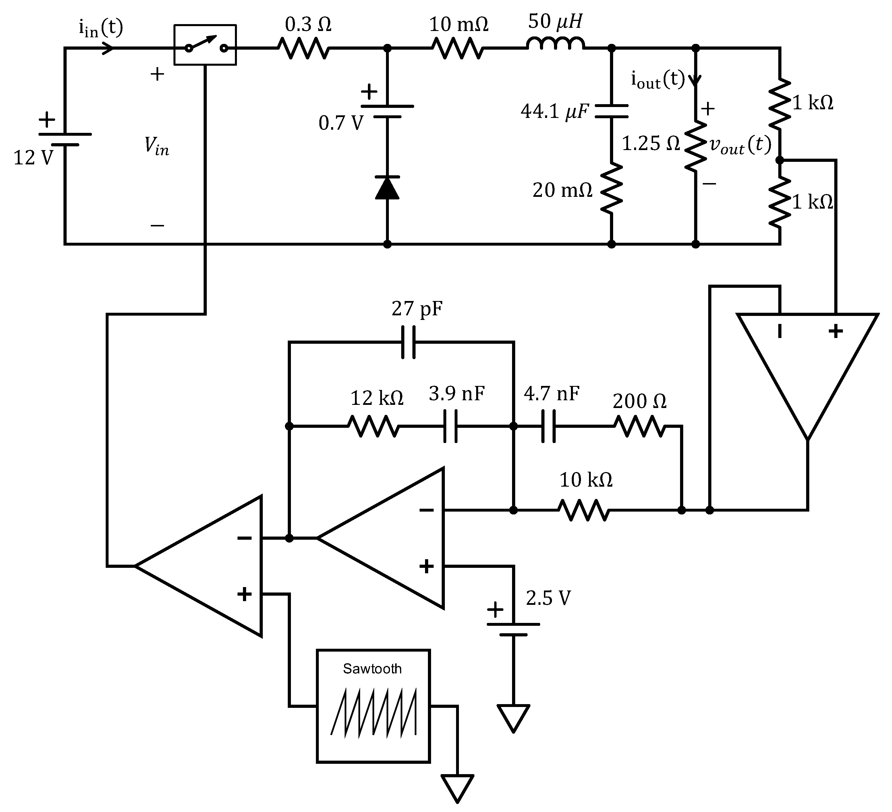
The AL technique presented in the previous section has been applied for the uncertainty quantification of the DC efficiency $\eta$, of the switching buck converter shown in Figure 1, as a function of seven parameters (i.e., $d=7$). Specifically, the values of the 12 V DC voltage source, the 50 μH inductor and its 10 mΩ equivalent series resistance (ESR), the 44.1 μF capacitance and its 20 mΩ ESR, the 1.25 Ω load resistance and the 0.3 Ω switch resistance have been modeled as seven uncorrelated Gaussian variables centered at their nominal values with standard deviations of 20% of their means. The above scenario has been implemented as a parametric netlist in LTSpice (additional details are provided in [6]). The resulting model will be used as the computational model in the following analysis.

The AL sampling technique presented in Section 2 is applied to build a surrogate model for the prediction of the converter efficiency. The algorithm starts with $n_0$ training samples provided by the computational model and selected via a standard LHS. Then, the AL method is used to select the new candidate points in the parameter space, and to compute, along with the computational model, the corresponding training responses. The iterative algorithm stops when a the maximum number of training samples $n_{max}$ is reached. For the sake of simplicity, in the following results $n_0=\lfloor 2n_{max}/3\rfloor$.

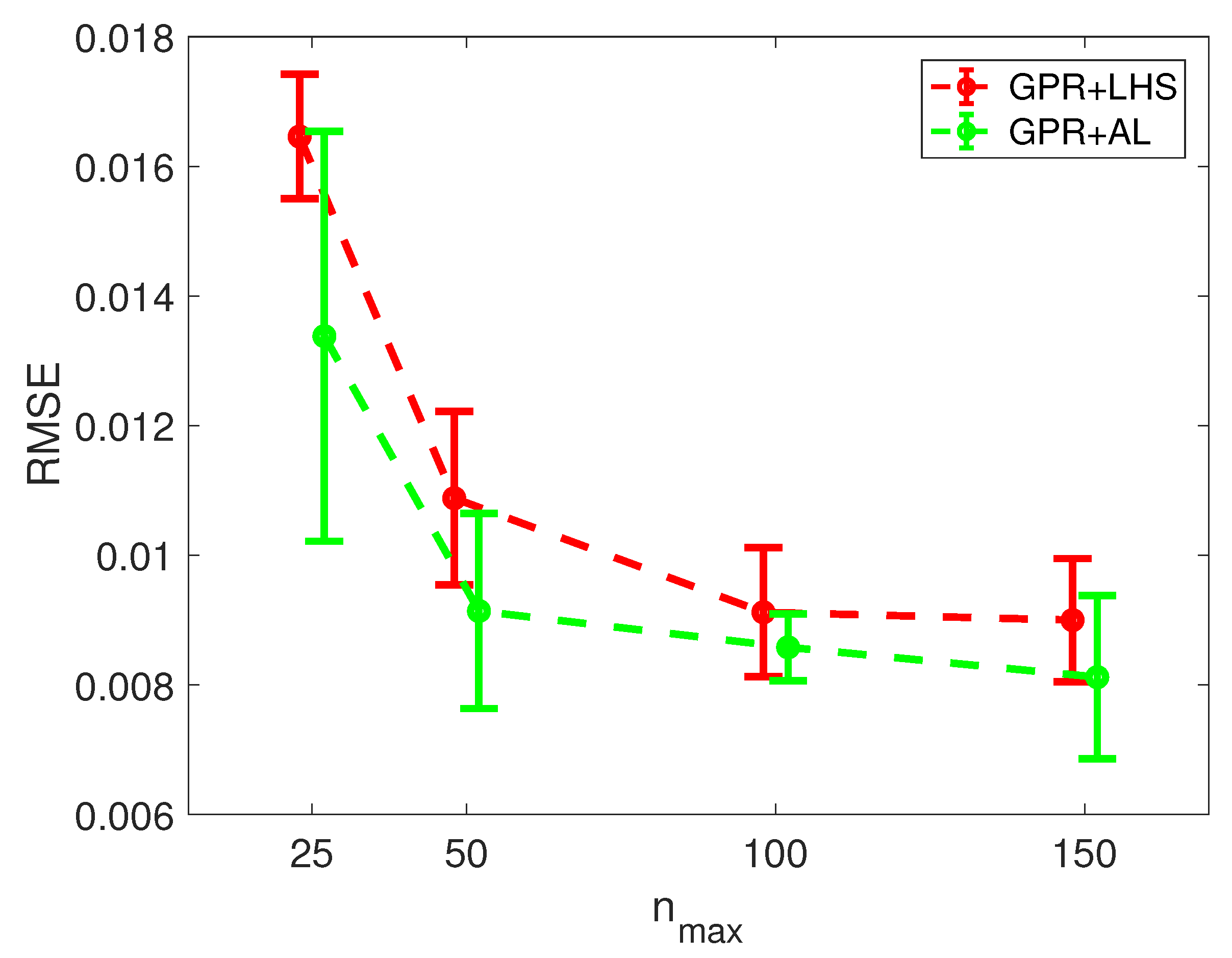
The performance of the surrogate mode GPR + AL, in which the GPR is combined with the AL, has been investigated for an increasing number of training samples, $n_{max}$ = 25, 50, 75 and 100, by considering the root-mean-square error (RMSE) computed between the model predictions and the corresponding results provided by a MC simulation with 10,000 samples. The obtained results are then compared with the ones predicted by an equivalent GPR-based model, called GPR + LHS, in which the training samples were selected via a plain LHS scheme. Since the accuracy of the resulting surrogates necessarily depends on the specific training samples used to build them, five different realizations of the training set are considered for each size $n_{max}$.

Figure 2 shows the results of the above comparison in terms of mean values (red and green dots) and standard deviations (red and green bars) of the RMSE computed by considering 5 different realizations of the training set for each size $n_{max}$. The results clearly highlight the improved accuracy of the proposed GPR + AL model with respect to the plain GPR surrogate. In fact, the mean values of the RMSE computed for the GPR + LHS surrogate are always lower than the corresponding ones obtained with the the equivalent GPR + LHS surrogate, thereby highlighting the benefits of the proposed AL strategy.

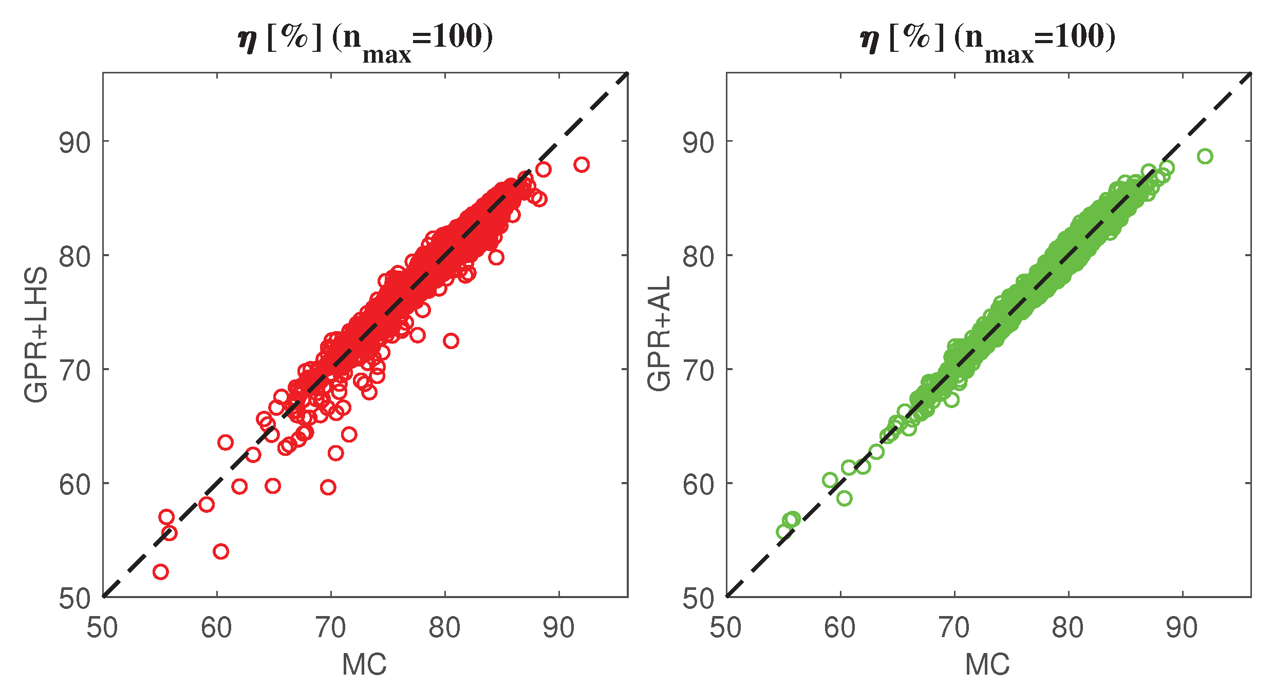
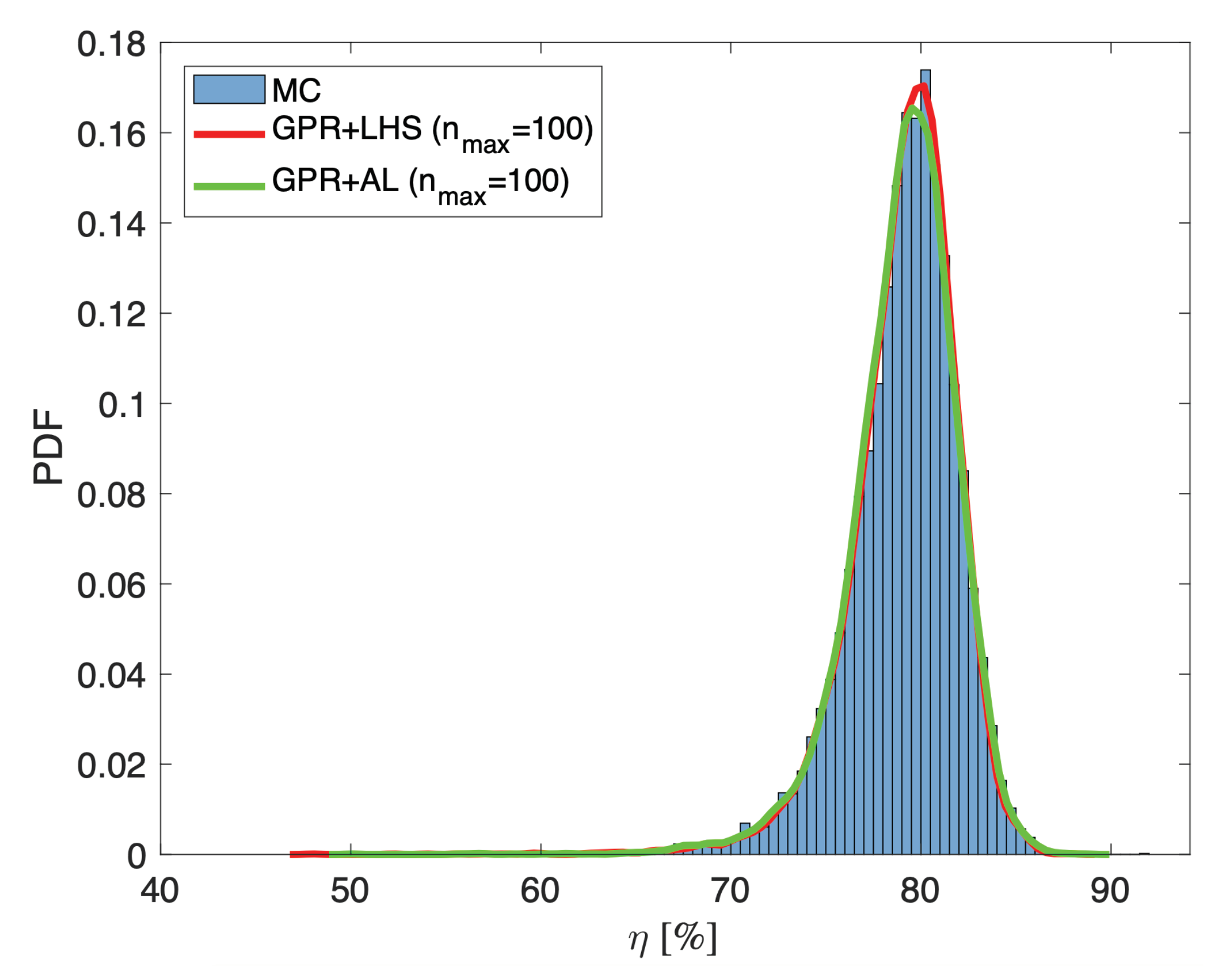
For the sake of illustration, Figure 3 and Figure 4 show the scatter plots and the pdfs calculated from the predictions of proposed AL+GPR surrogate and the ones of the GPR + LHS surrogate for a single set of $n_{max}=100$ training samples, again by using as reference the results of a 10,000 samples MC simulation with the computational mode. The plots confirm the capability of the two surrogate models of providing an accurate prediction of the actual behaviors of the converter efficiency. Additionally, Figure 5 shows an additional comparison between the $99\%$ CI predicted by the two models for 15 validation samples randomly selected among the samples used for the MC simulation. According to the results, the two surrogate models allow one to accurately account for the uncertainty of the model predictions, since most of the validation samples fall within the CIs predicted by the probabilistic models.

4. Conclusions

This paper presented a preliminary version of an AL scheme. The proposed AL algorithm, developed for the GPR, has been adopted for the optimal selection of the training samples in order to construct an accurate surrogate model of the scalar output of interest. The proposed methodology has been applied for the construction of a surrogate model for the uncertainty quantification of the efficiency of a buck converter as a function of seven uncertain parameters. The performance of the resulting surrogate has been compared with that of an equivalent GPR-based surrogate model in which the training samples were selected via a standard LHS scheme. According to the results presented in this work, the proposed AL methodology can be considered as a promising candidate approach for the training selection. Additional investigations are needed in order to better understand the performance of such methodology in different test-cases and for different dimensionality of the parameter space; possible different kinds of non-linear input–output behaviors could also be considered.