Learning Curves: A Novel Approach for Robustness Improvement of Load Forecasting ^†

Abstract

In the age of AI, companies strive to extract benefits from data. In the first steps of data analysis, an arduous dilemma scientists have to cope with is the definition of the ’right’ quantity of data needed for a certain task. In particular, when dealing with energy management, one of the most thriving application of AI is the consumption’s optimization of energy plant generators. When designing a strategy to improve the generators’ schedule, a piece of essential information is the future energy load requested by the plant. This topic, in the literature it is referred to as load forecasting, has lately gained great popularity; in this paper authors underline the problem of estimating the correct size of data to train prediction algorithms and propose a suitable methodology. The main characters of this methodology are the Learning Curves, a powerful tool to track algorithms performance whilst data training-set size varies. At first, a brief review of the state of the art and a shallow analysis of eligible machine learning techniques are offered. Furthermore, the hypothesis and constraints of the work are explained, presenting the dataset and the goal of the analysis. Finally, the methodology is elucidated and the results are discussed.

1. Introduction

The advent of electricity markets and the progress in Renewable Energy Sources (RES) have changed the nature of electricity production and consumption [1]. In order to increase the RES share and to use energy more effectively, energy system flexibility needs to be improved, for example, by means of enabling the demand-side management [2]. In this framework, electricity load prediction is required as an essential part in the energy industry to manage load fluctuations and aleatory RES [3]. Load forecasting is a useful and practical tool for efficient energy management, safer grid operation, and optimal maintenance planning. An accurate load forecasting is a key element to improve the environmental impact, sustainability, and cost-effectiveness of smart grids.

Electricity load prediction is vitally essential for the industries in deregulated economics [3]; load forecasting is necessarily implemented in Energy Management Systems (EMS) that optimally control appliances. An increasing number of numerical approaches has been proposed for energy prediction. A lot of models have been used and a coarse clustering is usually adopted in review articles: Statistical models, time series analysis, Machine Learning (ML), and Deep Learning (DL) [1,3]. Wei et al. [4] propose a review of data-driven approaches for the prediction and classification of buildings energy consumption; a comparison among white-box, grey-box, and black-box approaches for predicting consumption is described. White-box models lean on a complete knowledge of the physics of the systems while black-box models are completely data-driven and require historical data. Grey-box models are a hybrid solution between the other two. The paper focuses on data-driven models and, above all, describes Artificial Neural Networks (ANNs), Support Vector Machines (SVMs), and statistical regression. Yildiz et al. [5] cover the same subject, indeed they emphasize the broad application of ANNs and SVMs but, moreover, also Auto-Regressive (AR) models are cited; in particular the Auto-Regressive Integrated Moving Average (ARIMA) is defined as one of the most used techniques in load forecasting. In the latest years, by means of a greater computational power, many researchers started to apply Deep Learning techniques in order to improve load forecasting precision: Zhang et al. [6] details a variety of DL models like Restricted Boltzmann Machines (RBMs), Deep Belief Network (DBN), and RNN (Recurrent Neural Networks). Another novel algorithm taken into consideration is Extreme Gradient Boosting (XGBoost) that couples great performance with low execution time.

A plethora of researchers focused on model selection and hyper-parameters optimization; Khalid et al. [7] classify optimization methods for algorithm hyper-parameters in two groups: Nature-inspired approaches and statistical methods.

Recently, many companies have developed EMS whose services are based on data collection and artificial intelligence algorithms; load forecasting represents one of the most implemented service. Hence when an EMS business model is developed, a crucial point is the available amount of data. Once the model for prediction is selected, finding the trade-off between the volume of data and goodness of forecast is still a challenge. If the appropriate volume of training data can be coupled with the forecasting algorithm, the EMS has a robust load forecasting model. This aspect could be of great interest among companies developing services based on ML routines; indeed, when implementing an intelligent platform in a customer plant, estimating the monitoring period needed to collect data is significant to build an efficient business model. A powerful tool to tackle this estimation is to build Learning Curves (LCs).

A learning curve shows the measure of predictive performance on a given domain as a function of the training sample size. Reviewing learning curves of models can be used to diagnose problems with learning, such as underfitting or overfitting, as well as whether the training and validation datasets are suitably representative. Building an overly complex model leads to high variance error in prediction, but a too simple model has a high bias error. The opportunity of training the model with the proper number of observations leads to finding the architecture with an optimal trade off between variance and bias errors [8]. Although the learning curves are promising, in the literature they have been mainly applied to other types of data, with non correlated observations [9,10,11,12]. Hence in this context, the present work tries to bridge this research gap applying the learning curves procedure to time series.

The remainder of the paper is structured as follows. Section 2 presents a state of the art on Learning Curves and a background for this analysis. Proposed methodology is described in Section 3 and Section 4 presents results and discussion. Finally, conclusions are provided in Section 5.

2. State of the Art

Learning curves aim to compare the generalization performance of an algorithm as a function of training-set size. A learning curve shows the validation and training score of an estimator for different numbers of training samples. It is a tool to find out how much the estimator benefits from adding more training data and whether it suffers more from a variance error or a bias error [13]. Over two decades ago in machine learning research, the analysis of learning curves was a widespread tool for comparisons of Machine Learning techniques [14]; nowadays, it is rarely presented. Moreover, time-series LCs are not commonplace mainly because procedure presents some issues [15].

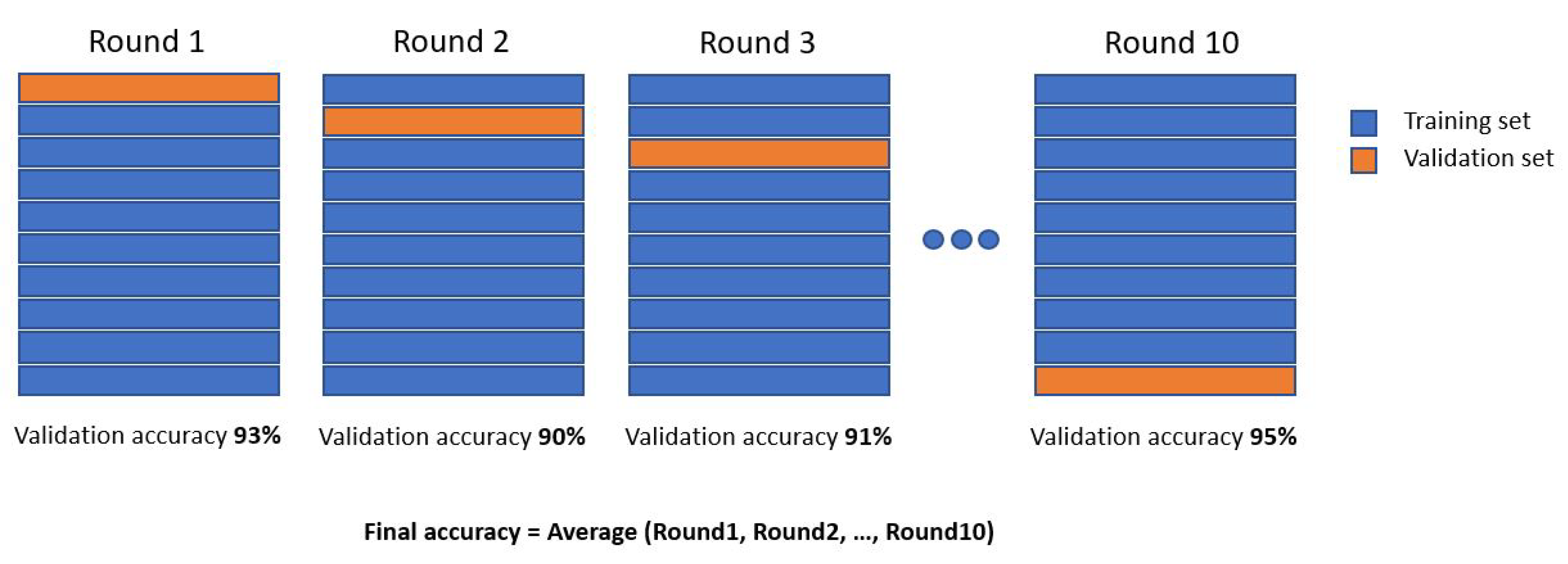
A common procedure for building LCs is implemented in the function named learning_curve of scikit-learn [13], a mainstream Python library. The just mentioned learning_curve function needs an estimator, the number of training observations that will be used to generate the LC, and the number k of fold to split data while using the k-fold validation strategy. This strategy splits the whole dataset k times, each time a different train-set and validation-set are extrapolated (Figure 1).

k-fold validation is a particular type of cross-validation (CV), a validation technique for assessing how the results of a statistical analysis will generalize on an independent dataset. Subsets of the training-set, whose size will be incremented after each k-fold validation, will be used to train the estimator and a score for each training subset size and for the test-set will be computed. Afterwards, the scores will be averaged over all k runs; in the end, two over-k-runs averaged score (both for train and test) will be obtained for each training subset size [13].

In the literature, there is not an extensive discussion of the LC subject. Most of the articles dealing with it refer to different fields of application. Ning et al. [12] test how the performance of Deep Convolutional Neural Networks (DCNNs) are affected by the size of the training-set in an image segmentation task: Six training-sets are considered and the performance of the DCNN trained with the larger dataset is used as the baseline. Zhu et al. [16] investigate the question of whether existing object recognition detectors will continue to improve as data grows, or saturate in performance due to limited model complexity. Beleites et al. [9], Figueroa et al. [10], and Hess and al. [11] study the importance of LCs in classification problems applied to the biomedical field where it is very difficult to obtain big datasets for training the estimator. All these analyses take into account independent samples, this means that the training-set can be enlarged, shuffled, and split without considering the samples order. However, this hypothesis is not valid when dealing with time-series.

Several strategies have been proposed in the literature for performance estimation of time-series and currently there is no consensual approach [17]. Out-of-Sample (OOS) approaches hold out a test-set in order to test a model on a never-seen portion of data. Train/test split can be faced with a different procedure: Sliding window or growing window [18]. OOS methods always retain the temporal order to guarantee the preservation of correlation among observations. In order to produce a robust estimation of predictive performance, Tashman [19] recommends applying OOS strategies in multiple test periods. Thus, by using OOS, the benefits of CV, especially for small datasets, cannot be exploited [20]. In general, CV is a common strategy both for model selection and for testing the generalization performance of an algorithm [21]. A fundamental hypothesis of CV is independence and identical distribution (i.i.d.) among observations. However, time-series has serial correlation in the data, possible non-stationarities, and time ordering, which forces not to use future data to predict the past; consequently the application of CV to time-series is not straightforward. There are several revised CV approaches designed for time-series; a wide review is presented from Bergmeir et al. [22]. Most common procedures are blocked CV and hv-block CV. Blocked CV has no initial random shuffling of data, and divides observation in K blocks as in k-fold CV; time order is kept within each block, although is broken across them [18]. h-block CV is a non-dependent cross-validation, as it leaves out the possibly dependent observations and only considers data points that can be considered to be independent [20].

Cerqueira et al. [18] compare different approaches on both stationary and non-stationary time-series. They conclude that CV procedures are suitable for stationary time-series but are not compliant with real data and with potential non stationarities; thus, OOS applied in multiple testing periods is recommended. Süzen et al. [15] present a procedure for time-series learning curves based on reconstructive CV; it combines OOS estimation and imputation of missing data at random by means of techniques like Kalman filtering [23].

3. Proposed Methodology

In this section, the building of learning curves is explained. As mentioned above, a cross-validation method is applied in a learning curves procedure in order to select the optimal number of observations needed for training a forecast algorithm. The aim of the proposed procedure is to present an adaptable methodology that can cope with all types of algorithms and all types of time-series data. The proposed methodology consists of three main steps: Data collection, algorithm selection, and building of learning curves. All these stages are described in the following sections.

3.1. Data Collection

When approaching a problem of energy load forecasting, the first activity to be performed is represented by data collection. Even if, lately, the words artificial intelligence and big data are mainstream, this does not mean that every facility manager arranges a data storage routine. Often data are monitored by means of a local Human-Machine-Inteface (HMI) by maintenance operators, whose goal is to check real-time behavior of the plant without a compulsory need of heaping data in an accessible structure.

Usually, many kinds of features can affect the energetic behavior of a plant and they can be grouped in the following short list:

•

Field measurements like energy consumption or plant temperatures. These signals are collected by a field device (e.g., a PLC or a remote I/O);

•

Management details like hotel reservations or hospital occupants. These numbers are collected by ERP softwares or, in the worst case, by hand-written registers;

•

Weather measurements and forecasts like external temperature or wind speed. These values are collected by weather stations or directly downloaded from the web.

All the above-mentioned data must be aggregated in a central entity whose task is to forward an average value to a database located in cloud or in a local server. The real importance of each measurement and its correlation with the load to be predicted is strictly dependent on the plant’s use case; when the monitored plant satisfies the energetic needs of a hotel then it is very useful to acquire for example the rooms reservation, the meeting room usage, and the external weather. Otherwise, when the building under investigation is a parking lot, it is helpful to know the period of the year and the parking spots occupation. A third example is represented by a manufacturing factory where the most important Key Performance Indicator (KPI) is the produced quantity of goods. In the real world, the machine learning engineer in charge of developing the ad-hoc model to predict energy load forecasting will not have access to all these information; most of the time model inputs will consist of the date and external temperature. Another important feature of data shape is granularity: In Italy, the energy market regulator [24] imposes to work with values averaged every hour or, in some cases, every 15 min. In order to maintain generality, in this paper measured signals are sampled every hour and the considered features are the most likely to be available: Date, external temperature and, of course, energy load consumption.

3.2. Algorithms Selection

When discussing forecasting, it is crucial to define the time interval to be forecasted; as Hammad et al. list in [25] there are four types of forecasting horizon:

•

Long-Term Load Forecasting (LTLF), time interval ranges from one year to 20 years ahead;

•

Medium-Term Load Forecasting (MTLF), time interval ranges from a week up to a year;

•

Short-Term Load Forecasting (STLF), time interval ranges from one hour to a week;

•

Ultra/Very Short-Term Load Forecasting (VSTLF), time interval ranges from a few minutes to an hour ahead and is used for real-time control.

In this paper, the goal is to predict the energy load forecasting of the next day, so it is a STLF problem. This assumption is not a required hypothesis for the methodology proposed in Section 3.4. As briefly introduced in Section 2, in the latest 40 years many methods have been developed and used for time-series forecasting and, in particular, for energy STLF. Makridakis et al. in [26] make a coarse division between statistical and ML methods; this kind of grouping method is widely used and, more in-depth forecasting model can be detailed as follows: Statistical Methods, ML Methods, and DL Methods.

• Statistical Methods are historically the most used because of their easy implementation and fast execution, and among these ARIMA and Holt–Winter methods are very popular. These approaches usually work better when dealing with low-frequency signals and when the target variable understays the hypothesis of time-invariance: Both statements are not compliant with the object of this paper.
• Machine Learning Methods had great promise at the beginning of 21st century and represent a good trade-off between performance and computational costs. Among the ML group, in this paper three techniques have been selected: Support Vector Regressor (SVR) because it is the most simple and understandable algorithm, Extreme Gradient Boosting (XGBoost) [27] because it is a novel algorithm able to outperform state-of-the-art techniques in many competitions, and Multi-Layer Perceptron (MLP) because it is often used as a load forecasting benchmark.
• Deep Learning Methods and in particular Recurrent Neural Networks (RNNs) could act as a central character in the short-term energy load forecasting because of their affinity with time-series and their well-known high performance; on the other hand, the hard hyper-parameter tuning phase risks a change in the focus of the work. Indeed, in order to face the LCs subject, it is important to train models with pre-selected hyper-parameters whose value can be considered correct by the authors with a high confidence degree.

3.3. Hyper-Parameters Selection

When building ML models to proceed with the LCs methodology, a strict hypothesis must be met: All hyper-parameter’s values must be tuned and then fixed to a defined value. In other words, optimization routines like randomized search [28] or grid search are not compliant.

In Section 3.2, the selected techniques used in this paper have been introduced: SVR, XGBoost, and MLP. Below, an extensive description of the settled hyper-parameter is reported.

The first algorithm selected is SVR; the SVR Scikit-learn library [29] has been used and four parameters have been tuned:

•

$C=1$, the regularization parameter;

•

$epsilon=0.1$, the epsilon-tube within which no penalty is associated;

•

$kernel=$ ’rbf’, the kernel type to be used in the algorithm;

•

$\gamma =0.08$, the kernel coefficient.

The second algorithm taken into analysis is XGBoost; the Scikit-learn Wrapper interface for XGBoost [30] has been implemented and four parameters have been tuned:

•

$max\_depth=4$, maximum tree depth for base learners;

•

$learning\_rate=0.1$, boosting learning rate;

•

$\lambda =1$, regularization term on weights;

•

$n\_estimators=100$, the number of gradient boosted trees.

The third developed algorithm is a two-layer MLP; the Scikit-learn library for MLP [31] has been exploited and four parameters have been tuned:

•

$hidden\_layer\_sizes=8$, one hidden layer with 8 neurons;

•

$activation=$ ’relu’, activation function for the hidden layer;

•

$\alpha ={10}^{-7}$, regularization term;

•

$batch\_size=1$, size of minibatches for stochastic optimizers.

3.4. Building of Learning Curves: The Proposed Methodology

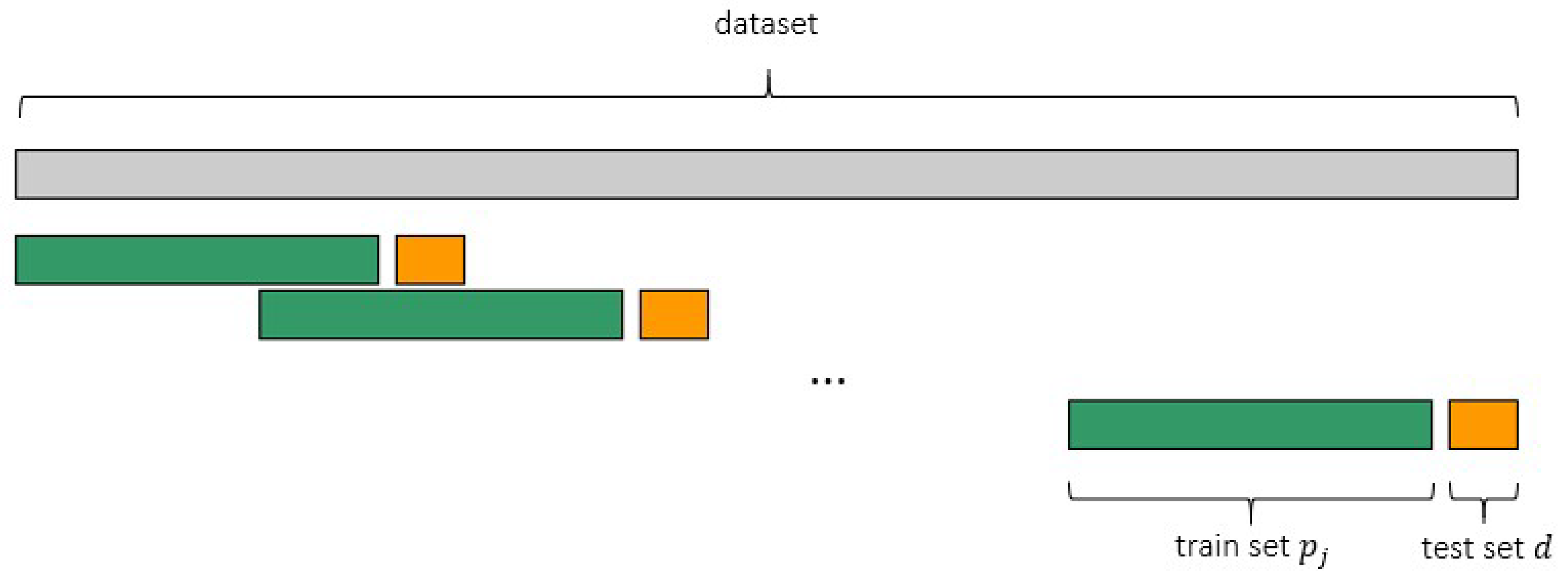
As underlined in Section 3.1, a multivariate time-series with n independent variables and only one dependent variable is analyzed with each observation of an independent time-series being $x\in {\mathbb{R}}^n$ and observations of dependent target variable are $y\in \mathbb{R}$. At time $t_i\in {\mathbb{R}}_0^{+}$, $x\left(t_i\right)$, and $y\left(t_i\right)$ represent the observations of independent and dependent variables; $t_0$ is considered as the first time sample available in the dataset. In this specific case, y is the time-series for energy load. A list of training-set size to test have to be defined since the generalization performance have to be shown as a function of the training-set size. The training-set size list has q elements; each $p_j$ with $j\in [1,...,q]$ is a training-set size. The test-set size d is fixed to a constant value and does not vary during the whole learning curves procedure. As cited in Section 3.2, the testing period considered in this work has a one-day length because the aim is a day-ahead load prediction. Moreover, the day of test immediately following the training-set is adopted. This is not a lack of generality, rather a different size for test-set can be applied and can be shifted from the end of training-set, as long as time order is retained.

By means of an OOS approach, a part of available data is used to fit the model, a different part to test it and assess the performance of the prediction algorithm. This procedure is repeated for each training-set size in the aforementioned list.

If $p_j$ is the training length, a set of $p_j$ consecutive observations is used for training the model and the following set of length d is used for testing purposes. The analyzed sets are:

$$\begin{array}{c}\hfill x\left(t_i\right)\le x\le x(t_i+p_j)\\ \hfill y\left(t_i\right)\le y\le y(t_i+p_j)\end{array}$$

and the test-set, if d is length for testing, is:

$$\begin{array}{c}\hfill x(t_i+p_j+1)\le x\le x(t_i+p_j+1+d)\\ \hfill y(t_i+p_j+1)\le y\le y(t_i+p_j+1+d).\end{array}$$

In order to produce a robust estimation of forecasting performance, for the same $p_j$ length of training, this strategy is applied in multiple test periods with a sliding window approach (Figure 2). It is worth underlining that, as the methodology is conceived, whenever the test-set is shifted, the training-set slides.

A statistically significant k number of tested days has to be chosen. In the period from $t_0+p_j$ to the end of the multivariate time-series, k tested days are chosen in a uniformly distributed and random way. The selection of k should be a trade off between the maximum $p_j$ training size and the possibility of testing an heterogeneous number of data portions also according to seasonality and trend in the time-series. Since in the present work one year of data is available, $k=30$ is enough to evaluate the algorithm generalized performance; this number of tested days allows to mitigate the sensitivity of error to different phases of a business cycle. Every time a sliding window is tested a metric has to be evaluated in order to compute y forecasting error for both the training-set and test-set. Different metrics can be used as a performance indicator, i.e. Root Mean Squared Error (RMSE) or Mean Absolute Error (MAE); they all have different shortcomings and merits. Mean Absolute Percentage Error (MAPE) has been used since it is scaled to the original y value and gives an intuitive interpretation of error. MAPE, for training of the m-th day is expressed by the formula:

$$MAP{E}_{m,train}=\sum _{i=1}^{p_j}\frac{\left|y_i^m-{\widehat{y}}_i^m\right|}{y_i^m}$$

(1)

where $y_i^m$ is the actual value and ${\widehat{y}}_i^m$ is the forecast value. For training, for example, it is computed over all the $p_j$ observations of the training set. The aforementioned procedure is performed k times for each $p_j$ training set size obtaining k MAPE error values for testing and k reconstruction errors of training. The average value $e_k$ of MAPEs for testing and training is reported in a learning curve graph. For training MAPE is computed as:

$$e_{k,train}=\frac{1}{k}\sum _{m=1}^{k}MAP{E}_{m,train}.$$

(2)

For the testing MAPE, the procedure is the same, but it is computed over d time-steps of the testing set as follows:

$$e_{k,test}=\frac{1}{k}\sum _{m=1}^k\sum _{i=1}^d\frac{\left|y_i^m-{\widehat{y}}_i^m\right|}{y_i^m}.$$

(3)

To plot the learning curves, the mean value of training errors and the mean value of test errors are taken; accordingly only two error scores for each training set size are plotted. Moreover, in order to show the scatter of data, the variance of error for both the training and testing curve is depicted by means of a colored shade.

Further details are reported in the implementation code available at [32].

4. Discussion and Results

In this work the proposed procedure is applied to the “ASHRAE-Great Energy Predictor III” competition data [33]; in particular, one year of hourly sampled data of a parking building (building id: 1215) has been selected. The target dependent variable is the electric load and the independent variables are:

• The time of the day as a cyclical variable (sine and cosine);
• The day of the week one-hot encoded;
• The month of the year as a cyclical variable (sine and cosine);
• The outdoor air temperature.

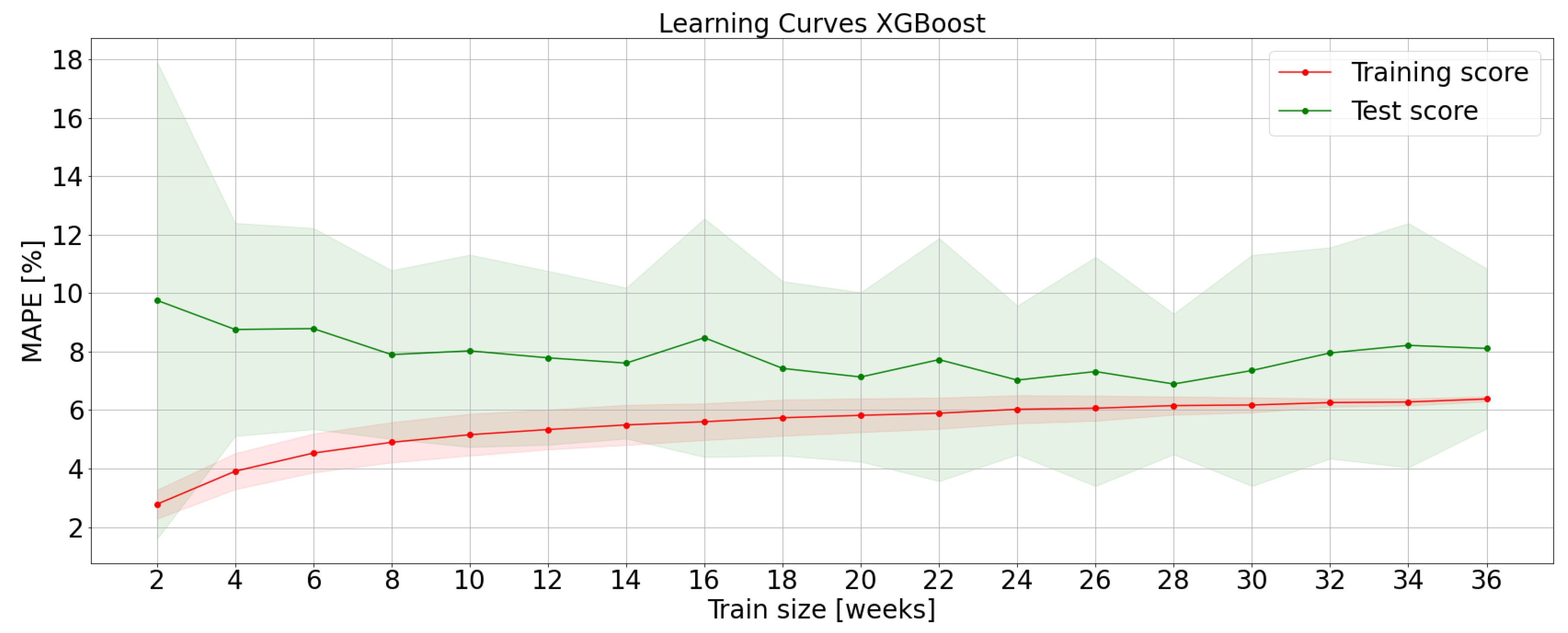
The training sizes $p_j$ range from 2 weeks to 36 weeks within a span of 2 weeks.

Figure 3 shows LCs obtained with the XGBoost algorithm. When the training-set size is small, the training error is lower since the information variance to be learnt is tiny. As a consequence, the model has no generalization capability and its test error is high. When the training set size increases, training MAPE increases and test MAPE decreases. Adding training data helps to reduce bias error. Training and test curves are very close between 20–28 training weeks. This narrow gap shows a low variance error: Training data are fitted well and the algorithm can generalize on unseen data. The gap increases for a training size higher than 28 weeks, which may indicate an overfitting problem. In this case, a training size of 24 weeks seems to be a good compromise for XGBoost.

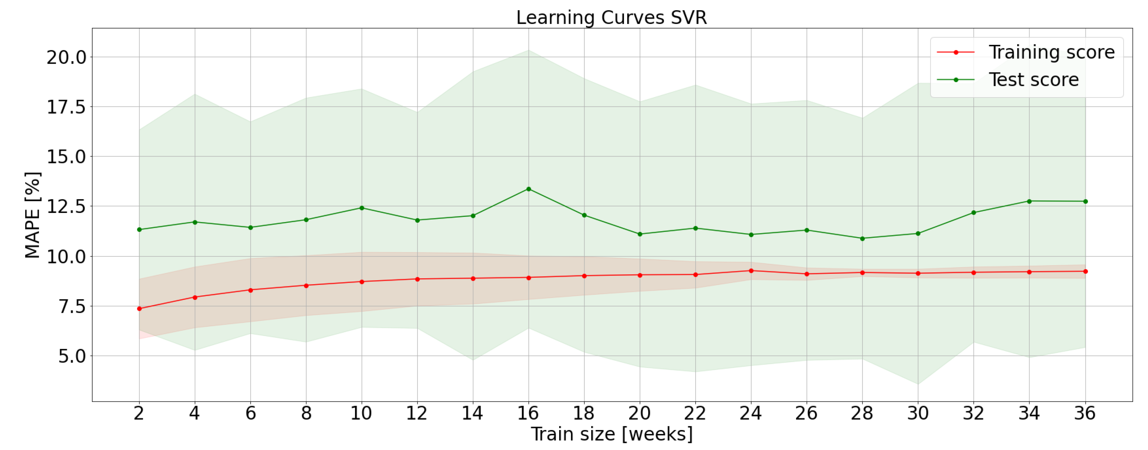
LCs for the SVR algorithm are shown in Figure 4. Bias error slightly but progressively decreases with a training set size; variance error reaches its minimum between 20 and 28 weeks. Hence, an appropriate training set size is 24 weeks.

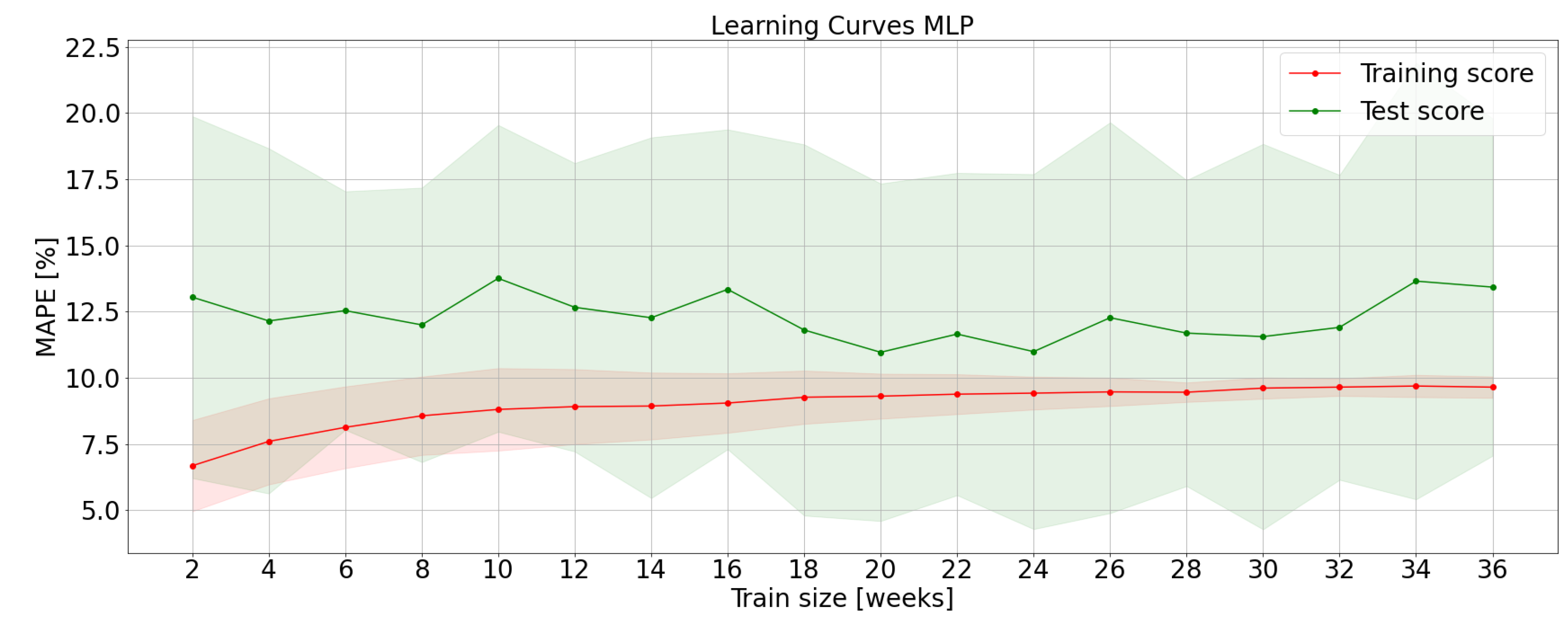
The same performance is presented from MLP whose LCs are plotted in Figure 5. Adding training data to small train dataset leads to increase the training error and decrease test error. This is mainly due to a reduction of bias error. The bias-variance dilemma is settled between 20 and 24 weeks of training. The appropriate training set size could be 20 weeks for MLP with two layers and hyperparameters as described in Section 3.3.

If learning curves are characterized by high training and test errors according to domain knowledge, the model may seem to suffer of a high bias error. Getting more training data will not help much. In this particular case, the desired MAPE is around 6%; while XGBoost reaches this target, SVR and MLP seem to suffer from underfitting. This problem highlights that SVR and MLP models have been tuned with simple architectures.

5. Conclusions

In this paper a procedure to analyze learning curves for time-series is presented; it aims to show a generalized performance of an algorithm with different training set sizes. The procedure retained time order and allowed to test heterogeneous samples for each training-set size. The performance estimation was analyzed in an Out-of-Sample approach with a sliding window. This methodology is suitable for real world data with potential non-stationarities. The developed procedure could be applied to any kind of data or algorithm.

The proposed methodology was applied to electrical load forecasting of a parking building. Learning curves were obtained with three different regression algorithms; namely XGBoost, SVR, and MLP. This analysis underlines how learning curves could give information about training and test as a function of a training set size and how to choose an appropriate size of data to cope with the bias-variance problem.

The full code is available at [32] in order to guarantee the reproducibility of the presented procedure.

As a next step, this research could be used as a tool for evaluating the estimator architecture by using different sets of hyperparameters to build LCs guides to understand their impact on the learning process.

References

- El-Hawary, M.E. Advances in Electric Power and Energy Systems-Load and Price Forecasting; IEEE Press Wiley: Piscataway, NJ, USA, 2017. [Google Scholar]
- D’Ettorre, F.; De Rosa, M.; Conti, P.; Testi, D.; Finn, D. Mapping the energy flexibility potential of single buildings equipped with optimally-controlled heat pump, gas boilers and thermal storage. Sustain. Cities Soc. 2019, 50, 101689. [Google Scholar] [CrossRef]
- Ahmad, T.; Zhang, H.; Yan, B. A review on renewable energy and electricity requirement forecasting models for smart grid and buildings. Sustain. Cities Soc. 2020, 55, 102052. [Google Scholar] [CrossRef]
- Wei, Y.; Zhang, X.; Shi, Y.; Xia, L.; Pan, S.; Wu, J.; Han, M.; Zhao, X. A review of data-driven approaches for prediction and classification of building energy consumption. Renew. Sustain. Energy Rev. 2018, 82, 1027–1047. [Google Scholar] [CrossRef]
- Yildiz, B.; Bilbao, J.I.; Sproul, A.B. A review and analysis of regression and machine learning models on commercial building electricity load forecasting. Renew. Sustain. Energy Rev. 2017, 73, 1104–1122. [Google Scholar] [CrossRef]
- Zhang, L.; Wen, J.; Li, Y.; Chen, J.; Ye, Y.; Fu, Y.; Livingood, W. A review of machine learning in building load prediction. Appl. Energy 2021, 285, 116452. [Google Scholar] [CrossRef]
- Khalid, R.; Javaid, N. A survey on hyperparameters optimization algorithms of forecasting models in smart grid. Sustain. Cities Soc. 2020, 61, 102275. [Google Scholar] [CrossRef]
- Würsch, C. Bias-Variance-Tradeoff: Crossvalidation & Learning Curves. Available online: https://stdm.github.io/downloads/courses/ML/V06_BiasVariance-LearningCurves.pdf (accessed on 5 October 2020).
- Beleites, C.; Neugebauer, U.; Bocklitz, T.; Krafft, C.; Popp, J. Sample Size Planning for Classification Models. Anal. Chim. Acta 2013, 760, 25–33. [Google Scholar] [CrossRef] [PubMed] [Green Version]
- Figueroa, R.L.; Zeng-Treitler, Q.; Kandula, S.; Ngo, L.H. Predicting sample size required for classification performance. BMC Med. Inform. Decis. Mak. 2012, 12, 8. [Google Scholar] [CrossRef] [Green Version]
- Hess, K.R.; Wei, C. Learning Curves in Classification With Microarray Data. Semin. Oncol. 2010, 37, 65–68. [Google Scholar] [CrossRef] [Green Version]
- Ning, H.; Li, Z.; Wang, C.; Yang, L. Choosing an appropriate training-set size when using existing data to train neural networks for land cover segmentation. Ann. Gis 2020, 26, 329–342. [Google Scholar] [CrossRef]
- Pedregosa, F.; Varoquaux, G.; Gramfort, A.; Michel, V.; Thirion, B.; Grisel, O.; Blondel, M.; Prettenhofer, P.; Weiss, R.; Dubourg, V.; et al. Scikit-learn: Machine Learning in Python. J. Mach. Learn. Res. 2011, 12, 2825–2830. [Google Scholar]
- Perlich, C.; Provost, F.; Simonoff, J. Tree Induction vs. Logistic Regression: A Learning-Curve Analysis. J. Mach. Learn. Res. 2003, 4, 211–255. [Google Scholar]
- Süzen, M.; Yegenoglu, A. Generalised Learning of Time-Series: Ornstein-Uhlenbeck Processes. arXiv 2020, arXiv:1910.09394. [Google Scholar]
- Zhu, X.; Vondrick, C.; Fowlkes, C.C.; Ramanan, D. Do We Need More Training Data? Int. J. Comput. Vis. 2016, 119, 76–92. [Google Scholar] [CrossRef] [Green Version]
- Cerqueira, V.; Torgo, L.; Smailovič, J.; Mozetixcx, I. A comparative study of performance estimation methods for time series forecasting. In Proceedings of the 2017 IEEE International Conference on Data Science and Advanced Analytics (DSAA), Tokyo, Japan, 19–21 October 2017; pp. 529–538. [Google Scholar]
- Cerqueira, V.; Torgo, L.; Smailovič, J.; Mozetixcx, I. Evaluating Time Series Forecasting Models: An Empirical Study on Performance Estimation Methods. arXiv 2019, arXiv:1905.11744. [Google Scholar] [CrossRef]
- Tashman, L.J. Out-of-sample tests of forecasting accuracy: An analysis and review. Int. J. Forecast. 2000, 16, 437–450. [Google Scholar] [CrossRef]
- Bergmeir, C.; Hyndman, R.J.; Koo, B. A note on the validity of crossvalidation for evaluating autoregressive time series prediction. Comput. Stat. Data Anal. 2018, 120, 70–83. [Google Scholar] [CrossRef]
- Arlot, S.; Celisse, A. A survey of cross-validation procedures for model selection. Stat. Surv. 2010, 4, 40–79. [Google Scholar] [CrossRef]
- Bergmeir, C.; Benítez, J.M. On the use of cross-validation for time series predictor evaluation. Inform. Sci. 2012, 191, 192–213. [Google Scholar] [CrossRef]
- Kalman, R.E. A New Approach to Linear Filtering and Prediction Problems. J. Basic Eng. 1960, 82 (Series D), 35–45. [Google Scholar] [CrossRef] [Green Version]
- Gestore Mercati Energetici. Available online: https://www.mercatoelettrico.org/en/ (accessed on 5 April 2021).
- Hammad, M.A.; Jereb, B.; Rosi, B.; Dragan, D. Methods and Models for Electric Load Forecasting: A Comprehensive Review. Logist. Sustain. Transp. 2020, 11, 51–76. [Google Scholar] [CrossRef] [Green Version]
- Makridakis, S.; Spiliotis, E.; Assimakopoulos, V. The M4 Competition: 100,000 time series and 61 forecasting methods. Int. J. Forecast. 2020, 36, 54–74. [Google Scholar] [CrossRef]
- Chen, T.; Guestrin, C. XGBoost: A Scalable Tree Boosting System. In Proceedings of the 22nd ACM SIGKDD International Conference on Knowledge Discovery and Data Mining, San Francisco, CA, USA, 13–17 August 2016. [Google Scholar]
- Bergstra, J.; Bengio, Y. Random Search for Hyper-Parameter Optimization. J. Mach. Learn. Res. 2012, 13, 281–305. [Google Scholar]
- Support Vector Regression (SVR) Scikit-Learn Library. Available online: https://scikit-learn.org/stable/modules/generated/sklearn.svm.SVR.html (accessed on 5 April 2021).
- Scikit-Learn Wrapper Interface for XGBoost. Available online: https://xgboost.readthedocs.io/en/latest/python/python_api.html#module-xgboost.sklearn (accessed on 5 April 2021).
- Multi-Layer Perceptron (MLP) Regressor Scikit-Learn Library. Available online: https://scikit-learn.org/stable/modules/generated/sklearn.neural_network.MLPRegressor.html (accessed on 5 April 2021).
- Giola, C.; Danti, P. Learning-Curves. 2020. Available online: https://github.com/jolachi/learning-curves/ (accessed on 5 April 2021).
- ASHRAE-Great Energy Predictor III. Available online: https://www.kaggle.com/c/ashrae-energy-prediction (accessed on 5 April 2021).
Figure 1.
Example of k-fold validation with k = 10.
Figure 2.
Scheme of proposed methodology.
Figure 3.
Learning curves obtained with the XGBoost algorithm.
Figure 4.
Learning curves obtained with a SVR algorithm.
Figure 5.
Learning curves obtained with the MLP algorithm.
Publisher’s Note: MDPI stays neutral with regard to jurisdictional claims in published maps and institutional affiliations. |
© 2021 by the authors. Licensee MDPI, Basel, Switzerland. This article is an open access article distributed under the terms and conditions of the Creative Commons Attribution (CC BY) license (https://creativecommons.org/licenses/by/4.0/).
Share and Cite
MDPI and ACS Style
Giola, C.; Danti, P.; Magnani, S. Learning Curves: A Novel Approach for Robustness Improvement of Load Forecasting. Eng. Proc. 2021, 5, 38. https://0-doi-org.brum.beds.ac.uk/10.3390/engproc2021005038
AMA Style
Giola C, Danti P, Magnani S. Learning Curves: A Novel Approach for Robustness Improvement of Load Forecasting. Engineering Proceedings. 2021; 5(1):38. https://0-doi-org.brum.beds.ac.uk/10.3390/engproc2021005038
Chicago/Turabian StyleGiola, Chiara, Piero Danti, and Sandro Magnani. 2021. "Learning Curves: A Novel Approach for Robustness Improvement of Load Forecasting" Engineering Proceedings 5, no. 1: 38. https://0-doi-org.brum.beds.ac.uk/10.3390/engproc2021005038