
Automatic Hierarchical Time-Series Forecasting Using Gaussian Processes †


1
Faculdade de Engenharia, Universidade do Porto, 4099-002 Porto, Portugal
2
Faculty of Computer Science, Dalhousie University, Halifax, NS B3H 1W5, Canada
3
Faculdade de Ciências, Universidade do Porto, 4099-002 Porto, Portugal
4
Fraunhofer Portugal, AICOS and LIACC, 4099-002 Porto, Portugal
*
Author to whom correspondence should be addressed.
†
Presented at the Seventh International Conference on Time-Series and Forecasting, Gran Canaria, Spain, 19–21 July 2021.
Eng. Proc. 2021, 5(1), 49; https://0-doi-org.brum.beds.ac.uk/10.3390/engproc2021005049
Published: 9 July 2021
(This article belongs to the Proceedings of The 7th International Conference on Time Series and Forecasting)
Abstract
:Forecasting often involves multiple time-series that are hierarchically organized (e.g., sales by geography). In that case, there is a constraint that the bottom level forecasts add-up to the aggregated ones. Common approaches use traditional forecasting methods to predict all levels in the hierarchy and then reconcile the forecasts to satisfy that constraint. We propose a new algorithm that automatically forecasts multiple hierarchically organized time-series. We introduce a combination of additive Gaussian processes (GPs) with a hierarchical piece-wise linear function to estimate, respectively, the stationary and non-stationary components of the time-series. We define a flexible structure of additive GPs generated by each aggregated group in the hierarchy of the data. This formulation aims to capture the nested information in the hierarchy while avoiding overfitting. We extended the piece-wise linear function to be hierarchical by defining hyperparameters shared across related time-series. From our experiments, our algorithm can estimate hundreds of time-series at once. To work at this scale, the estimation of the posterior distributions of the parameters is performed using mean-field approximation. We validate the proposed method in two different real-world datasets showing its competitiveness when compared to the state-of-the-art approaches. In summary, our method simplifies the process of hierarchical forecasting as no reconciliation is required. It is easily adapted to non-Gaussian likelihoods and multiple or non-integer seasonalities. The fact that it is a Bayesian approach makes modeling uncertainty of the forecasts trivial.
1. Introduction
The problem of automatically forecasting large numbers of univariate time-series is commonly found in different businesses [1]. In this setting, the selection of the appropriate time-series model, estimation of its parameters, and computation of the forecasts have to be done without human intervention. These large collections of time-series often involve multiple time-series aggregated by groups, such as geography. In this case, the forecasts for the bottom-level-series are required to add up to the forecasts of the aggregated ones. This constraint is referred to as coherence, and the process of adjusting forecasts to make them coherent is called forecast reconciliation [2]. Our work focuses on automatically forecasting a set of these hierarchically organized time-series. The goal is to generate accurate predictions for both the individual series and for each of the aggregation levels. This is to be achieved while ensuring that the forecasts are coherent. Finally, our algorithm is intended to be applied to any time-series domain.
A common approach for this type of problem is to produce forecasts for all aggregation levels and then reconcile the forecasts using linear or non-linear models (e.g., [2,3,4]). This strategy is highly dependent on the forecasting method used, and it is a two-step process. We follow a different approach where our forecasting algorithm takes into account the hierarchical information when predicting the individual series. This means that we do not need to reconcile the forecasts afterwards.
We introduce a combination of additive Gaussian processes (GPs) with a hierarchical piece-wise linear function to estimate, respectively, the stationary and non-stationary components of the time-series. We define a flexible structure of additive GPs that are summed coherently for each element of a group. GPs allow us to model relevant time-series patterns, such as seasonality or noise as their additive components. Its additive nature contributes to capturing the potential nested information in the hierarchy while avoiding overfitting (one common problem with GPs). In the non-stationary component, we are interested in modeling the trend of the data and trend changes over time while also capturing potential hierarchical relationships (e.g., similar trend patterns in the same group). With these goals in mind, we define a hierarchical piece-wise linear function. We adapt the idea of multilevel models from Bayesian statistics to define hyperparameters shared across related time-series. This way, we are estimating parameters for each group and using them to inform the estimation of the individual ones, that is, the individual parameters are partially pooled towards the group mean. This results in forecasts for the trend of the bottom-level series that already take into account the behavior of the aggregated ones.
From our experiments, our algorithm is able to scale to, at least, hundreds of time-series. The estimation of the posterior distribution of the parameters can be challenging for datasets with this size. To be able to perform it at that scale, we used mean-field approximation [5], which is an automatic algorithm to perform Variational Inference (VI). We validated the proposed algorithm in two different real-world datasets, showing its ability to work with small and large datasets with typical trend and seasonal patterns varying between groups.
In summary, our contributions are:
- A new algorithm for hierarchical time-series forecasting that does not require any type of reconciliation;
- The definition of a flexible structure of hierarchical additive GPs. Additive GPs are used in statistical analysis [6], whereas we propose a formulation to adapt it to automatic hierarchical time-series forecasting;
- The combination of additive GPs with a hierarchical piece-wise linear function to model, respectively, the stationary and non-stationary components of hierarchical time-series;
- An automatic method that does not require expert intervention to be fitted to new data.
2. Related Work
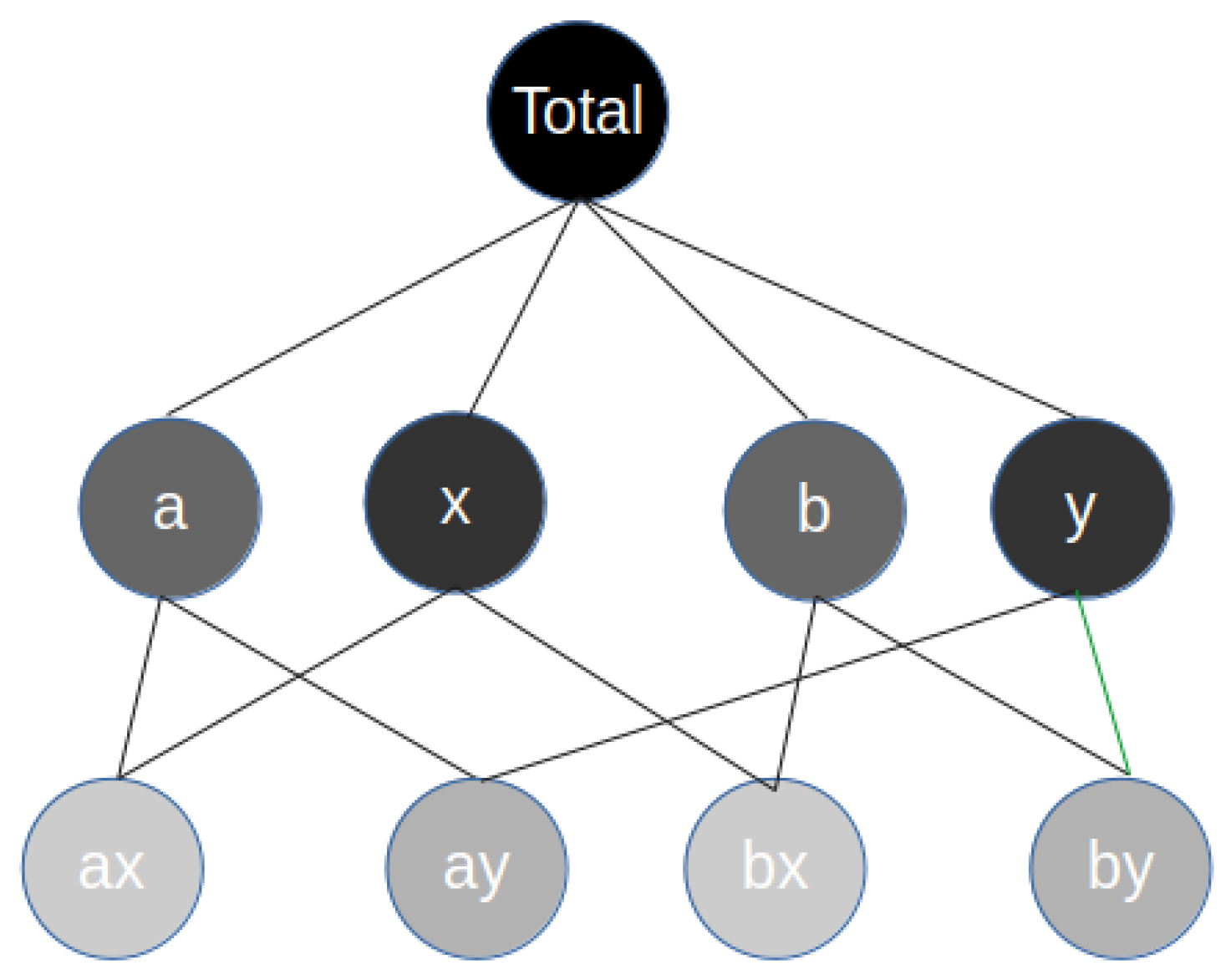
We work with a collection of s-related univariate time-series , where and denote the value of time-series i at time t. The time-series are aggregated by groups; in fact, each time-series is associated with an element l of every group g present in the dataset. We use vector of size s to encode this information. It has value 1, when the series s belongs to the element l of the group g, and 0, otherwise. To give a simple example, consider a dataset with two groups (g1 and g2), each one with two different elements (a and b, and x and y, respectively). We start with the most aggregated level of the data z. We can aggregate the individual series by group g1, forming the series , and by its elements, forming and . We can do the same for the second group g2, forming series , or by its elements, and . At the bottom level, this would generate four different series (i.e., , ). Figure 1 illustrates a particular example of this dataset.
The goal of forecasting is to predict the next time-steps for all time-series, that is, .
where are the parameters of the model. For any given time-series i, we refer to time-series as target time-series, as the training range, and to time as the prediction range. The time-point is referred to as the forecast start time and is the forecast horizon. Point forecasts for a given time-series, i at time are denoted by , and the point forecast errors are denoted by .
2.1. Time-Series Forecasting
When we consider the automatic forecasting process of a single time-series and include constraints such as integer or single seasonality, the state-space exponential smoothing (ETS) [7] and automated ARIMA [1] procedures are still considered state-of-the-art approaches. When we extend to non-integer or multiple seasonalities, there are other methods which become relevant, including TBATS [8] or Prophet [9]. In the case of Prophet, there is also additional flexibility on how the trend is modeled. Traditional GPs do not excel in automatic forecasting. An adaptation with benchmark forecasting resulting in single univariate time-series has been proposed [10], but prior knowledge was introduced to achieve that competitiveness. There are several challenges when using GPs to do automatic forecasting, namely, the lack of a criterion for kernel selection and the long time required for training different competing kernels. On the other hand, Recurrent Neural Networks (RNN) are gaining popularity as an alternative to statistical methods. Nevertheless, the settings where they can achieve competitiveness are still very narrow and require user adaptation (see [11] for an extensive study on the topic).
Forecast accuracy is usually measured by summarizing the forecast errors using a scaled metric, such as the Mean Absolute Scaled Error (MASE) (see [7] for an extended overview on forecast error metrics). For seasonal time-series, a scaled error can be computed by:
and MASE is defined by .
2.2. Hierarchical and Grouped Time-Series
When working with related time-series, the focus is to model cross-series information to improve univariate models. There are cases where the time-series are only related by belonging to the same domain ([12]), while in other cases they can be aggregated in groups or in a hierarchy. There are different methods designed to work with hierarchical time-series. The method initially proposed by [13] and improved in [2,14] consists in optimally combining and reconciling all forecasts at all levels of the hierarchy. A linear regression is used to combine the independent forecasts, guaranteeing that the revised forecasts are as close as possible to the independent forecasts but maintaining coherence. These works were further extended to allow a non-linear combination of the base forecasts [3] and adapted to a Bayesian setting [4]. A Bayesian approach takes into account the uncertainty across all levels of the hierarchy to obtain the revised forecasts.
In a different direction, [15] introduced a Bayesian hierarchical state-space model, which used shared hyperpriors over regression coefficients and latent process characteristics. Thus, the series-level parameters were inherited from global parameters which are shared across all time-series.
2.3. Gaussian Process
In a GP, we directly infer a distribution over functions. Each function can be seen as a random variable assigned to a finite number of discrete training points X and any finite number of these variables have a joint Gaussian distribution. More formally, the GP is completely specified by its mean and covariance functions:
The mean function is usually kept at zero, as the covariance is often flexible enough to model most of the data patterns.
2.3.1. Kernels
The kernels define the types of functions that we are likely to sample from the distribution of functions [16]. We can then draw samples from the distribution of functions evaluated at any number of points, that is, . They can be separated into stationary kernels, such as the squared exponential kernel (RBF), the periodic kernel (PER) and the white noise kernel (WN) and non-stationary ones, such as the linear kernel (LIN). The stationary kernels can be written as
where represent the variances, are the length-scale parameters which control the smoothness, c defines the offset, and p is the period. The is the Kronecker delta, which has the value of one for , and zero otherwise.
2.3.2. Predictions
When we are predicting using GPs, we are interested in the joint distribution of the training outputs and the test outputs . For most of the applications, we are faced with approximate function values, since there is noise to be considered in the form of . Assuming additive-independent and identically distributed Gaussian noise with variance , the joint distribution of the observations and the function values at the test positions can be written as
where denotes the matrix evaluated at all pairs of training (n) and test points (). Finally, we can derive the conditional distribution [16],
.
2.4. Variational Inference
Variational inference is an alternative to Markov Chain Monte Carlo for fitting Bayesian models. It provides a deterministic solution computed in a shorter time, potentially less accurate, as it is an approximation. It approximates the true distribution with a simpler distribution (usually Gaussian) , easier to sample from and evaluate. It is called variational density and is parameterized by . To calculate the distance between these two distributions, the Kullback–Leibler (KL) divergence can be used. Directly minimizing the KL divergence is difficult, but there is an easier and equivalent way to solve this problem, which is by maximizing the evidence lower bound (ELBO). It can be written as
There are several methods to maximize the ELBO that usually require model-specific calculations. The algorithm Automatic Differentiation Variational Inference (ADVI) was proposed by [5] to automate this task. An important thing to notice is that the consequence of choosing to use a mean-field Gaussian for the variational approximation is that it does not capture the correlations between parameters. On the other hand, the full-rank Gaussian variational approximation is able to capture them but the computational cost can be prohibitive.
3. Hierarchical Model
3.1. Hierarchical Structure
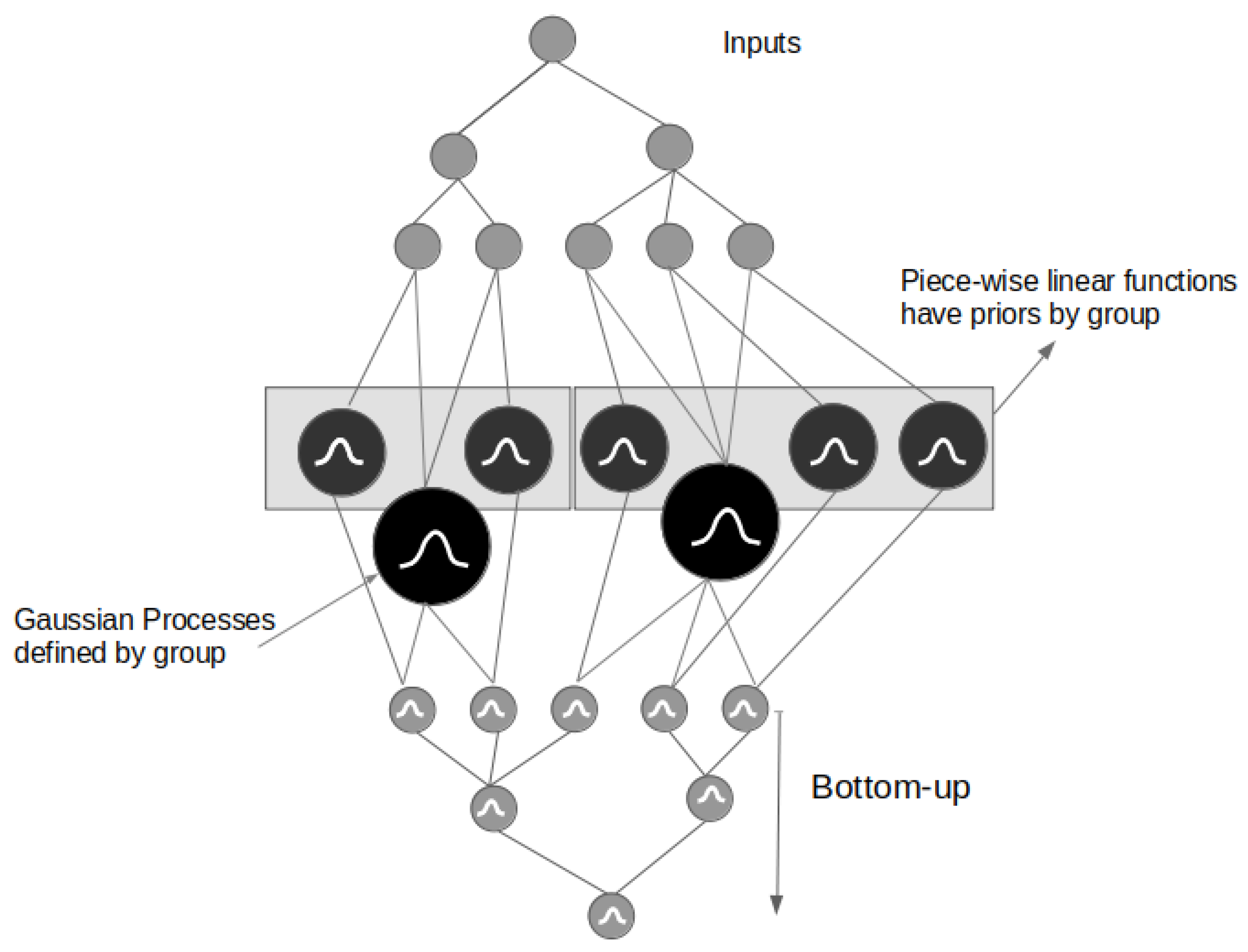
As we saw in Section 2.2, our work is focused on datasets that have a hierarchical or grouping structure, and thus, there is potential information nested in those substructures of the data. We defined the two main components of our model: The GP is used to capture seasonality, irregularities and noise, while the trend is modeled using a piece-wise linear model. We denote our algorithm by Hierarchical Piece-Wise Linear GPs (HPLGPs). An illustrative representation is introduced in Figure 2.
To leverage the nested information in each group or hierarchy of our data, we modeled an individual GP per element of each group, where g represents a group from the set of groups G and represents the elements of the specific group g. This way, we were able to model the most important features present in each element of a group, something that we could not do if we have directly modeled each time-series with an individual GP.
Before fitting our hierarchical model, we standardized each time-series to have mean 0 and variance 1. We defined a Normal likelihood for our target variable .
For its mean value, we summed the result of the piece-wise linear function with the sum of the GPs, defined by . Recall that we are using to encode the information of what series belong to the element l of group g. We used to ensure that we are summing our GPs coherently for each element of a group.
Thus, we have a number of GPs equal to the number of elements in every group. However, in order to narrow the learning process inside each group, the hyperparameters are only defined per group and not per group element. Notice that we reparameterized following the algorithm described in [16], as it is more efficient. We can denote the GPs as:
where are the different kernels defined by group (covered in-depth in Section 3.2). We add a piece-wise linear function to the result of the GPs in the likelihood of our model, defined by:
where k is the growth rate, is the rate adjustments, m is the offset parameter, and ensures that the function is continuous (this formulation is covered in-depth in Section 3.3). Notice that we have one parameter for each series s and change point c. We will not be focusing on the effect change of using a different number of change points, nor on the automatic selection of the number of change points. Nevertheless, it is possible to address this problem with the current formulation. If one chooses a large number of potential points and uses a sparse prior on the parameter, it is the equivalent to performing a L1 regularization.
The approximation of our parameter distributions is performed using ADVI, introduced in Section 2.4.
3.2. Gaussian Processes
In designing our GPs, the goal was to define a set of kernels that is flexible enough to be used in different settings. The combination of kernels that we used included the squared exponential kernel (RBF), the period kernel (PER) and the white noise kernel (WN). The equations for each kernel were presented in Section 2.3.1. The RBF kernel was selected to model medium term non-linear irregularities in the data. We could have used a more complex kernel, such as the rational quadratic kernel, but from our experiments, we did not see any relevant improvement and so we avoid adding more parameters to the model. The choice of priors for the length-scale parameters, for both the RBF and PER kernels, needs some attention. First, one important thing to be aware when optimizing the parameters of the kernels are the correlations between them. For instance, the length-scale has a strong interaction with other parameters. The same happens between kernels. The usage of more informative priors on the hyperparameters helps to mitigate (but not erase) that problem. Secondly, the data do not inform length-scales larger or shorter than the maximum or minimum covariate distance. In our case, the distance between points is always one, while the maximum distance is equal to the number of time-points in each series. Thus, we used an inverse gamma with mass inside this interval because it suppresses both zero and infinity. Both and are defined as , where n is the number of data points in the training set.
To model the main seasonal pattern of the data we selected a PER kernel. Since we define a prior over the period p, we just need to be careful with the range of probable values for p. For instance, with weekly data we just need to ensure that our distribution has a significant amount of mass around 52 and we let the algorithm infer the value that best fits our data. In other models, we often need to be precise and define weeks in a year. The period is a non-negative parameter, for which we could have chosen a distribution that ensures non-negativity, such as a Gamma distribution. As we defined a very informative prior, we decided to use a Laplace distribution , where D is the main seasonality pattern found in the data.
We also specified a noise model with a simple WN kernel. This kernel gives us the capacity to absorb short term irregular behaviors without compromising the fit of the other kernels. It also helps stabilize our covariance function. Once again, we need to use a very informative prior for , to avoid losing valid information which could be modeled as noise.
Finally, we can write our covariance function as:
where , , , , p, and are all the hyperparameters to learn. As a final note to our kernel design, our algorithm can be trivially extended to have multiple seasonalities. This is useful when there is a weakly seasonality pattern in the data aside from the main pattern. It can be done by adding a new component to our covariance function. A second periodic kernel can be added on and the prior for its period p can be defined in the expected range of values for the specific seasonality.
3.3. Trend Model
At this point, it is important to notice that we only used stationary kernels. Our algorithm would not be capable to forecast most of the known time-series datasets, since we would not be able to model the trend component. In the case of ARIMA models, the process consists of performing a first differencing on the data and then fitting an ARMA model. We tested the inclusion of a non-stationary kernel, the linear kernel LIN, to model the trend of the data. Nonetheless, the results were not convincing enough. On one hand, the RBF and LIN kernels were in some cases catching some of the same effects. The necessary regularization to overcome this problem was somewhat customized to the dataset in usage, not easy to generalize. We believe that this was also a consequence of the hierarchical structure that we defined for the GPs. On the other hand, some datasets had non-linear trends or regime changes, which we were unable to catch using a linear kernel. We could also model the trend as the mean of the GPs, but, once again, the results were not as convincing as the option that follows.
We decided to model the trend of the data using a piece-wise linear model, following the definition in [9]. The trend changes are modeled by the definition of a set of change points at times , and a vector of trend adjustments , where is the change in rate that occurs at time . The rate at any time-point t is then the base rate k, plus all the adjustments up to that point. This can be represented by a matrix A of size , such that
Finally, we cover the prior distributions of the parameters of the piece-wise linear model. To also leverage the group information when estimating the trend of the different series, we defined a hierarchical structure for these parameters. This is also called partial pooling because, while we define individual parameters for each series, they are sharing information through a hyperprior. This has a shrinking effect on the estimations, that is, we assume that the parameters k, m and come from a normal distribution centered around their respective group mean , and , with a certain standard deviation , or . We only present here the hierarchical structure for as it is similar to k and m,
4. Results
We chose datasets with different characteristics to ensure that our algorithm is able to capture strong trend and seasonal patterns that vary across groups, while working with either small or large numbers of series.
The first dataset used is fairly small and it represents the quarterly Australia prison population evolution over the period 2005Q1-2016Q4. It has 32 time-series, each one having 48 time-points. We tested with different values for but only present here the scenario where as it was consistent with the other experiments. It comprises three groups: The six states and two territories of Australia (we will refer these two also as states for simplification), the gender of the prisoner (male or female) and the legal status (whether prisoners have already been sentenced or not). Despite its size, there is an interesting change of rate of growth in the data of some groups. We can see that the algorithm behaves rather well even with a small amount of data to be trained on. We used two different models as a benchmark (see Table 1). First, we simply fitted individual GPs to each single series and then aggregate these upwards to produce revised forecasts for the whole hierarchy (usually referred as bottom-up method). The second is the optimal reconciliation algorithm MinT proposed by [2].
The second dataset is larger (304 time-series) and comprises the monthly number of visitors in Australia from 1998–2016. We used the first 204 time-points to train our algorithm and the last 24 to evaluate its performance. This dataset can be disaggregated in four different groups. The first three are purely hierarchical and concern the geographical nature of the data: 8 states, 27 zones and 76 regions. The purpose of travelling is a different group that contains four different elements. The total number of elements in groups is 114 which means that we fitted 114 GPs. These data have a strong yearly seasonal pattern and, in specific groups, there are particular trend patterns. Once again, we can see in Table 2 that our algorithm is able to not only capture the relevant patterns in individual series but also to capture the nested ones within groups, specially in the most aggregated level of the hierarchy.
5. Conclusions and Future Work
We proposed an algorithm for automatic hierarchical time-series forecasting. Our results show that it can compete with its statistical counterparts, being able to effectively capture the behaviors of the aggregated level series while not losing accuracy on the individual ones. Our algorithm is easily extensible, for instance, to work with non-Gaussian likelihoods or multiple seasonality patterns.
As future work, the increase of the scalability of the model can be developed further if we consider approximation methods, such as sparse approximations (e.g., [17]). Another interesting point to address is the posterior distributions correlations of our parameters. There are several works (e.g., [18,19]) on low-rank approximations to the covariance matrix to capture some of these correlations.
In the interest of reproducible science, our proposed algorithm is publicly available (https://github.com/luisroque/automatic_hierarchical_forecaster, last accessed 29 June 2021).
Funding
This work was partially funded by the Canada Research Chairs program, a Discovery Grant from NSERC, and by the project Safe Cities - Inovação para Construir Cidades Seguras, with the reference POCI-01-0247-FEDER-041435, co-funded by the European Regional Development Fund (ERDF), through the Operational Programme for Competitiveness and Internationalization (COMPETE 2020), under the PORTUGAL 2020 Partnership Agreement.
Data Availability Statement
Publicly available datasets were analyzed in this study. The data can be found here: https://github.com/luisroque/automatic_hierarchical_forecaster, last accessed 29 June 2021.
References
- Hyndman, R.J.; Khandakar, Y. Automatic time-series forecasting: The forecast package for R. J. Stat. Softw. 2008, 26, 1–22. [Google Scholar]
- Wickramasuriya, S.L.; Athanasopoulos, G.; Hyndman, R.J. Optimal Forecast Reconciliation for Hierarchical and Grouped Time Series Through Trace Minimization. J. Am. Stat. Assoc. 2019, 114, 804–819. [Google Scholar] [CrossRef]
- Spiliotis, E.; Abolghasemi, M.; Hyndman, R.J.; Petropoulos, F.; Assimakopoulos, V. Hierarchical forecast reconciliation with machine learning. arXiv 2020, arXiv:2006.02043. [Google Scholar]
- Novak, J.; McGarvie, S.; Garcia, B.E. A Bayesian model for forecasting hierarchically structured time series. arXiv 2017, arXiv:1711.04738. [Google Scholar]
- Kucukelbir, A.; Tran, D.; Ranganath, R.; Gelman, A.; Blei, D.M. Automatic Differentiation Variational Inference. J. Mach. Learn. Res. 2017, 18, 1–45. [Google Scholar]
- Cheng, L.; Ramchandran, S.; Vatanen, T.; Lietzén, N.; Lahesmaa, R.; Vehtari, A.; Lähdesmäki, H. An additive Gaussian process regression model for interpretable non-parametric analysis of longitudinal data. Nat. Commun. 2019, 10, 1798. [Google Scholar] [CrossRef] [PubMed]
- Hyndman, R.; Athanasopoulos, G. Forecasting: Principles and Practice, 3rd ed.; OTexts: Melbourne, Australia, 2021. [Google Scholar]
- Livera, A.M.D.; Hyndman, R.J.; Snyder, R.D. Forecasting time-series With Complex Seasonal Patterns Using Exponential Smoothing. J. Am. Stat. Assoc. 2011, 106, 1513–1527. [Google Scholar] [CrossRef] [Green Version]
- Taylor, S.J.; Letham, B. Forecasting at Scale. Am. Stat. 2018, 72, 37–45. [Google Scholar] [CrossRef]
- Corani, G.; Benavoli, A.; Augusto, J.; Zaffalon, M. Automatic Forecasting using Gaussian Processes. arXiv 2020, arXiv:2009.08102. [Google Scholar]
- Hewamalage, H.; Bergmeir, C.; Bandara, K. Recurrent Neural Networks for time-series Forecasting: Current status and future directions. Int. J. Forecast. 2021, 37, 388–427. [Google Scholar] [CrossRef]
- Smyl, S. A hybrid method of exponential smoothing and recurrent neural networks for time-series forecasting. Int. J. Forecast. 2019, 36, 75–85. [Google Scholar] [CrossRef]
- Hyndman, R.J.; Ahmed, R.A.; Athanasopoulos, G.; Shang, H.L. Optimal combination forecasts for hierarchical time-series. Comput. Stat. Data Anal. 2011, 55, 2579–2589. [Google Scholar] [CrossRef] [Green Version]
- Athanasopoulos, G.; Ahmed, R.A.; Hyndman, R.J. Hierarchical forecasts for Australian domestic tourism. Int. J. Forecast. 2009, 25, 146–166. [Google Scholar] [CrossRef] [Green Version]
- Chapados, N. Effective Bayesian Modeling of Groups of Related Count time-series. In Proceedings of the 31st International Conference on Machine Learning, Beijing, China, 21–26 June 2014. [Google Scholar]
- Rasmussen, C.E.; Williams, C.K.I. Gaussian Processes for Machine Learning (Adaptive Computation and Machine Learning); The MIT Press: Cambridge, MA, USA, 2005. [Google Scholar]
- Quiñonero-Candela, J.; Rasmussen, C.E. A Unifying View of Sparse Approximate Gaussian Process Regression. J. Mach. Learn. Res. 2005, 6, 1939–1959. [Google Scholar]
- Ong, V.M.H.; Nott, D.J.; Smith, M.S. Gaussian variational approximation with a factor covariance structure. arXiv 2017, arXiv:1701.03208. [Google Scholar] [CrossRef] [Green Version]
- Guo, F.; Wang, X.; Broderick, T.; Dunson, D.B. Boosting variational inference. arXiv 2016, arXiv:1611.05559. [Google Scholar]
Figure 1.
Example of time-series aggregated by group.

Figure 2.
Simplified representation of our proposed algorithm. Notice that the GPs are defined by group, while the piece-wise linear functions are fitted to individual series (with priors defined by group). The model outputs coherent bottom-series forecasts which we can directly sum up (using a bottom-up strategy) to get the forecasts for the higher-level series.


Table 1.
Results (MASE) for the Australia prison dataset using .
| Algorithm | Bottom | Total | State | Gender | Legal | All |
|---|---|---|---|---|---|---|
| HPLGPs | 2.09 | 0.244 | 1.628 | 0.518 | 2.682 | 1.885 |
| BU-GPs | 2.319 | 1.626 | 1.638 | 1.396 | 2.813 | 2.242 |
| MinT | 2.06 | 0.895 | 1.698 | 0.907 | 1.84 | 1.96 |
Table 2.
Results (MASE) for the Australia tourism dataset using .
| Algorithm | Bottom | Total | State | Zone | Region | Purpose | All |
|---|---|---|---|---|---|---|---|
| HPLGPs | 1.082 | 0.779 | 1.128 | 1.014 | 0.981 | 0.981 | 1.018 |
| BU-GPs | 1.211 | 1.271 | 1.312 | 1.211 | 1.122 | 1.121 | 1.196 |
| MinT | 0.906 | 1.27 | 1.07 | 0.893 | 0.895 | 1.04 | 0.897 |
Publisher’s Note: MDPI stays neutral with regard to jurisdictional claims in published maps and institutional affiliations. |
© 2021 by the authors. Licensee MDPI, Basel, Switzerland. This article is an open access article distributed under the terms and conditions of the Creative Commons Attribution (CC BY) license (https://creativecommons.org/licenses/by/4.0/).
Share and Cite
MDPI and ACS Style
Roque, L.; Torgo, L.; Soares, C. Automatic Hierarchical Time-Series Forecasting Using Gaussian Processes. Eng. Proc. 2021, 5, 49. https://0-doi-org.brum.beds.ac.uk/10.3390/engproc2021005049
AMA Style
Roque L, Torgo L, Soares C. Automatic Hierarchical Time-Series Forecasting Using Gaussian Processes. Engineering Proceedings. 2021; 5(1):49. https://0-doi-org.brum.beds.ac.uk/10.3390/engproc2021005049
Chicago/Turabian StyleRoque, Luis, Luis Torgo, and Carlos Soares. 2021. "Automatic Hierarchical Time-Series Forecasting Using Gaussian Processes" Engineering Proceedings 5, no. 1: 49. https://0-doi-org.brum.beds.ac.uk/10.3390/engproc2021005049