Fuzzy Prediction Intervals Using Credibility Distributions  ^†

Abstract

We present a new forecasting scheme based on the credibility distribution of fuzzy events. This approach allows us to build prediction intervals using the first differences of the time series data. Additionally, the credibility expected value enables us to estimate the k-step-ahead pointwise forecasts. We analyze the coverage of the prediction intervals and the accuracy of pointwise forecasts using different credibility approaches based on the upper differences. The comparative results were obtained working with yearly time series from the M4 Competition. The performance and computational cost of our proposal, compared with automatic forecasting procedures, are presented.

1. Introduction

This paper presents a new prediction scheme for time series using fuzzy logic and credibility distributions. Uncertainty about the future behavior of each time series is analyzed through the first and upper differences of the observed data, while the last raw observation is maintained as the level of the time series. That is, we assume that the uncertainty is not in the observed data, but in the underlying processes of the relationship between the data of the time series.

The uncertainty about the future of the time series is approximated using fuzzy variables [1]. Thus, working with fuzzy variables enables us to build prediction intervals with a given credibilistic coverage and provide pointwise forecasts through the credibility expected value, using various fuzzy prediction models. This credibility approach has not been previously proposed in the context of time series, although approximation of the uncertainty of fuzzy events using fuzzy variables is well established in other knowledge areas.

In previous works, we dealt with fuzzy variables to approximate the uncertainty of the future returns on assets or the return of a given portfolio [2,3]. In this paper, we propose to predict the future performance of the times series using LR-type fuzzy variables, whose parameters are estimated by using the sets of differences of several orders of the observed data. Finally, the optimistic values of the fuzzy variable provide us with the prediction intervals for each nominal coverage.

It must be noted that this new approach does not follow the classical fuzzy time series methodology, suggested by Song and Chissom [4], which has subsequently been improved by other authors (for more details about fuzzy time series, see, e.g., [5] and references therein). Recently, we introduced a new weighted fuzzy-trend method to forecast a stock index, which outperforms Chen’s methodology [6] for pointwise one-step forecasting [7]. However, the aforementioned approach does not provide suitable tools for building accurate fuzzy prediction intervals and k-step-ahead forecasts.

The main goal of this research is to design new fuzzy prediction models for nonseasonal time series that provide fuzzy variables as forecasts of the future performance of the time series, using the historical datasets. The properties of the fuzzy variables and their credibility distributions are useful to obtain prediction intervals and accurate ex-post forecasts.

To further investigate the predictive behavior of our proposals and the accuracy of the outputs compared to other forecasting approaches, we applied them to a set of yearly time series from the M4 Competition [8]. For the comparison with automatic forecasting procedures, we selected the exponential smoothing (ES) and ARIMA procedures included in the forecast package for R [9], which is available in CRAN (https://cran.r-project.org/, accessed on 15 June 2021), by using the R commands ‘es’ and ‘auto.arima’, respectively.

The rest of the paper is structured as follows. Section 2 summarizes concepts and definitions of fuzzy theory. The proposed methodology for building prediction intervals and pointwise forecasts is formulated in Section 3. In Section 4, we analyze the numerical results obtained by the fuzzy prediction models for a dataset from the M4 Competition. Finally, we set out our conclusions in Section 5.

2. Uncertainty Estimation with Fuzzy Logic

Let us recall some useful definitions based on fuzzy logic. The possibility and necessity of every fuzzy event (for instance, $\{T\ge x\}$, for any $x\in \mathbb{R}$), where T is a fuzzy number, can be evaluated according to the possibility distribution associated with its membership function (${\mu }_T\left(t\right)$) as follows [10]:

$$Pos\{T\ge x\}=su{p}_{t\ge x}{\mu }_T\left(t\right),\mathrm{and}Nec\{T\ge x\}=1-su{p}_{t<x}{\mu }_T\left(t\right)$$

(1)

Thus, an alternative to quantify the uncertainty is the credibility measure introduced in [11]:

$$Cr\{T\ge x\}=\frac{1}{2}Pos\{T\ge x\}+\frac{1}{2}Nec\{T\ge x\},$$

(2)

A fuzzy variable $\xi$ is described by means of the following membership function,

$${\mu }_{\xi }\left(x\right)=min(1,2Cr\{\xi =x\}),x\in \mathbb{R},$$

(3)

whose credibility distribution ${\Phi }_{\xi }:\mathbb{R}\to [0,1]$ is defined as

$${\Phi }_{\xi }\left(x\right)=Cr\{\xi \le x\}=\frac{1}{2}(su{p}_{t\le x}{\mu }_{\xi }\left(t\right)+1-su{p}_{t>x}{\mu }_{\xi }\left(t\right)).$$

(4)

In particular, $\xi$ is said to be an L-R power fuzzy variable if its credibility distribution has the following form [2]:

$${\Phi }_{\xi }\left(x\right)=\left\{\begin{array}{cc}0& \mathrm{if} x\le l\\ \\ \frac{1}{2}[1-{\left(\frac{A-x}{A-l}\right)}^{\alpha }]& \mathrm{if} l\le x\le A\\ \\ \frac{1}{2}[1+{\left(\frac{x-A}{u-A}\right)}^{\beta }]& \mathrm{if} A\le x\le u\\ \\ 1& \mathrm{if} x\ge u\end{array}\right.$$

(5)

Throughout the paper, we denote LR-power fuzzy variables of this type by $\xi ={(l,A,u)}_{\alpha ,\beta }$. The estimation of the parameters of $\xi$ is made by means of sample percentiles of the dataset of differences between chronologically consecutive historical data.

Credibility Expected Values and Prediction Intervals

The pointwise estimation of a fuzzy variable $\xi$ is approximated by its credibility expected value, denoted by $E\left(\xi \right)$ [11]. For an LR-power fuzzy variable $\xi ={(l,A,u)}_{\alpha ,\beta }$, its expected mean is calculated as follows [2]:

$$E\left(\xi \right)=A+[\frac{1}{2}(u-A)\frac{\beta }{\beta +1}-(A-l)\frac{\alpha }{\alpha +1})]$$

(6)

Finally, it must be said that the prediction intervals can be built using the credibility distribution (5), calculating suitable $\gamma$-optimistic values of the fuzzy variable $\xi$, defined as follows [1]:

$${\xi }_{sup}\left(\gamma \right)=\{r:Cr\{\xi \ge r\}\ge \gamma \}.$$

(7)

Alternatively, the endpoints of one specific prediction interval, for instance, with a $\gamma 100\%$ of nominal coverage for $\gamma \in [0,1]$, can be directly calculated through the inverse function of the credibility distribution, ${\Phi }_{\xi }^{-1}(.)$, as follows:

$$I{P}_{\gamma 100\%}\left(\xi \right)=[{\Phi }_{\xi }^{-1}\left(\frac{1-\gamma }{2}\right),{\Phi }_{\xi }^{-1}\left(\frac{\gamma }{2}\right)].$$

(8)

3. New Fuzzy Prediction Methods

Let us consider a time series $Y\left(t\right)$, whose observed data are ${\left\{y_t\right\}}_{t=1}^N$, $y_N$ being the last observation. Then, we can build the k-order differences between consecutive observations, $k\ge 1$.

At time i, $i=1,\dots ,N-k$, let us define the k-difference, $d_i^k$, as the difference between the forward observation of k order from time i and the observation at time i, that is

$$d_i^k=y_{i+k}-y_i\forall i=1,\cdots ,N-k,k=1,\cdots ,N-i$$

(9)

Thus, for every k-order, $k\ge 1$, we calculate the time series of the k-differences:

$$D^k={\left\{d_i^k\right\}}_{i=1}^{N-k}.$$

(10)

We assume that the uncertainty about the future behavior of the time series $Y\left(t\right)$ can be estimated through the credibility approximation of the time series of the k-differences. To do so, we consider the LR-power fuzzy variable ${\mathsf{\Delta }}^k={(l,A,u)}_{\alpha ,\beta }$, whose credibility distribution is given in Equation (5), which is built using the sample percentiles $p_j$ of the set $D^k$. The bounded support of ${\mathsf{\Delta }}^k$ is approximated by $l=p_0$ and $u=p_{100}$, where $A=p_{50}$. The shape parameters are obtained as $\alpha =ln\left(0.5\right)/ln\left(\frac{A-p_{25}}{A-l}\right)$ and $\beta =ln\left(0.5\right)/ln\left(\frac{p_{75}-A}{l-A}\right)$, assuming that the sample percentiles $p_{25}$ and $p_{75}$ have a $50\%$ possibility of being realistic (see, e.g., [12] for more information about LR fuzzy numbers). The forecaster can choose other sample percentiles, if that decision could improve the approximation of ${\mathsf{\Delta }}^k$, avoiding outliers.

3.1. One-Step Ahead Fuzzy Forecast Model: FFM

For the time series $Y\left(t\right)=\{y_1,\cdots ,y_N\}$, let us consider the fuzzy variable ${\mathsf{\Delta }}^1$, which is built considering the set of the first differences, $D^1={\left\{d_i^1\right\}}_{i=1}^{N-1}$. Since $y_N$ is the last observation, the one-step ahead fuzzy forecast is defined as follows:

$$\widehat{F}(N+1)=y_N+{\mathsf{\Delta }}^1$$

(11)

That is, a translation of magnitude $y_N$ is applied to the fuzzy variable ${\mathsf{\Delta }}^1$ to build the one-step-ahead fuzzy forecast. Consequently, by applying the well-known property of the credibility expected mean ($E(a+\xi )=a+E\left(\xi \right)$, for $a\in \mathbb{R}$), the pointwise forecast is the credibility expected value ${\widehat{y}}_{N+1}=E\left(\widehat{F}(N+1)\right)=y_N+E\left({\mathsf{\Delta }}^1\right)$.

In order to provide further fuzzy predictions, we define the fuzzy variables for h steps ahead, $h\ge 2$, using those previously forecasted pointwise as

$$\widehat{F}(N+h)=E\left(\widehat{F}(N+h-1)\right)+{\mathsf{\Delta }}^1,$$

(12)

and obtain that $\widehat{F}(N+h)=y_N+(h-1)E\left({\mathsf{\Delta }}^1\right)+{\mathsf{\Delta }}^1$. Analogously, we obtain the pointwise forecasts as their credibility expected values: ${\widehat{y}}_{N+h}=E\left(\widehat{F}(N+h)\right)=y_N+hE\left({\mathsf{\Delta }}^1\right)$, for $h\ge 2$.

The prediction intervals for the h-step-ahead pointwise prediction, $h\ge 1$, are built following Equation (8) for the corresponding fuzzy variables $\widehat{F}(N+h)$.

3.2. K-Step-Ahead Fuzzy Forecast Model: FFKM

Let us consider the time series $Y\left(t\right)=\{y_1,\cdots ,y_N\}$, for which k-step-ahead forecasts are requested. For $1\le h\le k$, we build the fuzzy variables ${\mathsf{\Delta }}^h$, using the corresponding set of the h-order differences, $D^h={\left\{d_i^h\right\}}_{i=1}^{N-h}$, $h\ge 1$. Note that in this modeling approach we need to build k fuzzy variables, $\left\{{\mathsf{\Delta }}^h\right\}$ for $1\le h\le k$, depending on the ex-post predictions requested.

Let $y_N$ be the last observation; then, for every $1\le h\le k$, the h-step-ahead fuzzy forecast is defined as follows:

$$\widehat{F}(N+h)=y_N+{\mathsf{\Delta }}^h$$

(13)

The pointwise h-step-ahead forecast is then ${\widehat{y}}_{N+h}=E\left(\widehat{F}(N+h)\right)=y_N+E\left({\mathsf{\Delta }}^h\right)$, and the corresponding prediction intervals are built using the credibility distribution of every fuzzy variable $\widehat{F}(N+h)$, $1\le h\le k$.

In the context of fuzzy time series, other authors have also considered the differences of consecutive observations to introduce new forecasting methods [13,14], following the basic scheme introduced in [6]. However, their approaches do not have any element in common with the ones we propose in this paper.

3.3. A Numerical Example

Let us present the performance of our methods FFM and FFkM, using the first yearly time series from the M4 Competition [8]. This time series contains 31 observations, $N=31$. We make a partition of this observed data, in such a way that 28 first observations belong to the training set ($y_{28}$ = 7651.4), while the last 3 are reserved for the comparison with the pointwise h-step-ahead forecasts provided, h = 1, 2, 3.

3.3.1. Performance of the FFM Method

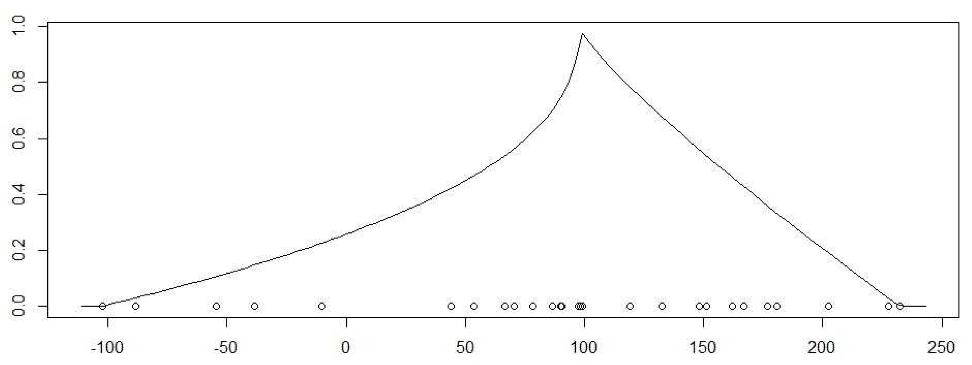
Using the aforementioned methodology for applying the FFM method, we build the fuzzy variable ${\mathsf{\Delta }}^1$, which is defined as ${\mathsf{\Delta }}^1={(-102.3,97.4,232.3)}_{0.41,0.84}$, the credibility expected value being $E\left({\mathsf{\Delta }}^1\right)$=98.93. Thus, ${\widehat{y}}_{29}$ = 7750.33.

Figure 1 shows the plot of the membership function of the fuzzy variable ${\mathsf{\Delta }}^1$. The observed first differences are plotted as small circles. Using the suitable sample percentiles of the first differences in $D^1$, we calculate the 90% prediction interval of $I{P}_{90\%}\left({\mathsf{\Delta }}^1\right)=[-79.0,226.6]$. Note that the credibility expected value of the fuzzy variable $E\left({\mathsf{\Delta }}^1\right)$ is not the middle point of this prediction interval.

The calculations of the corresponding h-step-ahead forecasts and the prediction intervals, for h = 2, 3, are easily obtained by taking into account both the properties of the expected value and the sample percentiles, $p_j(a+D^1)=a+p_j\left(D^1\right)$, for $a\in \mathbb{R}$. In particular, ${\widehat{y}}_{30}$ = 7849.26 and ${\widehat{y}}_{31}$ = 7948.20.

3.3.2. Performance of the FFKM Method

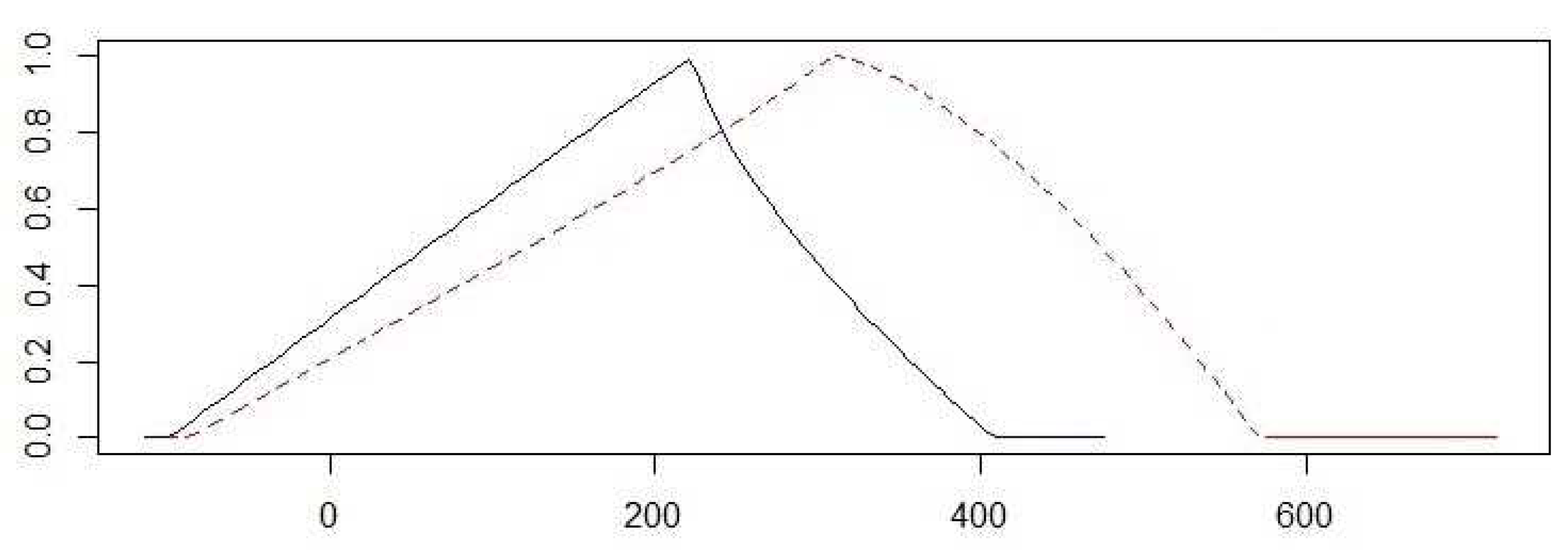
In order to determine the out-of-sample forecasts and their prediction intervals, we apply the FFkM method, for k = 3. It is easily seen that the first iteration is identical for both methods, FFM and FFkM. However, we need to build the sets of the second- and third-order differences to obtain the fuzzy variables ${\mathsf{\Delta }}^2$ and ${\mathsf{\Delta }}^3$, respectively. Figure 2 shows the membership function of the aforementioned fuzzy variables.

Table 1. Pointwise h-step-ahead forecasts obtained by applying the FF3M method, 90% prediction intervals and prediction errors, for h = 1, 2, 3.

	y(28 + h)	$\widehat{\mathit{y}}$(28 + h)	IP(90%)	Prediction Error
h = 1	7587.3	7750.3	[7572.4, 7878.0]	163.0
h = 2	7530.5	7831.3	[7568.4, 8053.0]	300.8
h = 3	7261.1	7944.0	[7585.4, 8202.7]	682.9

shows the raw observation, the pointwise forecasts obtained by applying the FF3M method, the 90% prediction interval and the prediction error, $e_h=\widehat{y}(N+h)-y(N+h)$, for h = 1, 2, 3.

Note that the trend changes in the observed data have not been suitably estimated by the proposed methods, so that the prediction error has increased when h increases. In fact, only the 90% prediction interval of the first step contains the actual observation. In the next section, we report the results obtained using our proposals for a large set of yearly time series.

4. Results

To investigate the predictive behavior of our fuzzy methods, also in comparison to standard automatic approaches, we applied them to a set of data from the M4 Competition [8]. This competition contains 100,000 seasonal and nonseasonal time series. The results of the M4 Competition have been globally published for each type of subset of time series, depending on their forecasting horizon.

We worked with the nonseasonal yearly time series. Since our proposals need a number of observations to build the fuzzy variables, a filter was applied to this set of 23,000 yearly series, that is, $N\ge 31$. We thus obtained a selection of 9060 yearly time series, with a range of observed sizes: $N\in$ [31, 700]. To carry out our study, we used the R language [15], applying various R functions in conjunction with some functions written by the authors.

For the comparison, we followed the specifications established for the M4 Competition and computed forecasts up to six steps ahead. Initially, until 31 May 2018, only the training set was available, but, once it was finished, the values to be forecasted were published in the R package M4comp2018. We also selected two automatic forecasting procedures available in the R package forecast, exponential smoothing (es) and auto.arima [9], for the comparison of both ex-post predictions and coverage of the prediction intervals. We also compared the average computational cost of obtaining these forecasts.

For every model $M_j=\{SE,ARIMA,FFM,FF6M\}$ and each time series, $Y_i\left(t\right)$ for $1\le i\le 9060$, the prediction errors were measured as follows:

$$e_{i,M_j}\left(h\right)={\widehat{y}}_{M_j(h,i)}-y_{(h,i)},h=1,\cdots ,6,j=1,\cdots ,4$$

(14)

${\widehat{y}}_{M_j(h,i)}$ being the forecast at h steps-ahead applying the $M_j$ method and $y_{(h,i)}$ being the observation at time $N+h$. The mean absolute percentage error (MAPE) and the symmetric mean absolute percentage error (sMAPE) were employed to measure forecasting accuracy, respectively:

$$MAP{E}_{M_j}\left(h\right)=100\ast \frac{1}{9060}\sum _{i=1}^{9060}\left[\frac{e_{i,M_j}\left(h\right)}{y_{(h,i)}}\right],h=1,\cdots ,6$$

(15)

$$sMAP{E}_{M_j}\left(h\right)=100\ast \frac{2}{9060}\sum _{i=1}^{9060}\frac{|e_{i,M_j}\left(h\right)|}{|{\widehat{y}}_{M_j(h,i)}+y_{(h,i)}|},h=1,\cdots ,6$$

(16)

For the comparison of the prediction intervals, wed use their empirical coverage, that is, the percentage of times that the observation in included in those intervals.

4.1. Prediction Intervals

Table 2. Comparison of the empirical coverage at each step ahead attained for every method. The last column shows the mean of the coverage as a percentage.

IP(80%)	E.1	E.2	E.3	E.4	E.5	E.6	Mean
SE	0.65	0.72	0.76	0.76	0.77	0.78	74%
ARIMA	0.51	0.53	0.56	0.56	0.56	0.57	55%
FFM	0.66	0.79	0.89	0.92	0.93	0.94	86%
FF6M	0.66	0.80	0.86	0.83	0.78	0.73	78%
IP(95%)
SE	0.81	0.87	0.89	0.89	0.88	0.89	87%
ARIMA	0.49	0.56	0.65	0.68	0.69	0.72	63%
FFM	0.74	0.86	0.93	0.95	0.96	0.96	90%
FF6M	0.74	0.87	0.93	0.91	0.86	0.83	86%

shows the results of the empirical coverage obtained by applying the different methods at each h-step ahead, denoted as $E.h$, for $h=1,\cdots ,6$, on the scale [0,1], for the 9060 yearly time series. Note that the nominal coverage is established in 80% and 95%, respectively. The last column shows the mean of the empirical coverage, as a percentage.

The results in Table 2 show that the prediction intervals provided by the FFM method are wider than those provided by FFkM method, while the coverage of the prediction intervals provided by FFkM is closer to that provided by exponential smoothing. The ARIMA procedure provided prediction intervals with lower empirical coverage.

The computational time was calculated in milliseconds for every run, that is, the elapsed time from when time series data were read until the six ex-post forecasts were given.

Table 3. Statistics of computing times for forecasting the 9060 yearly time series.

Milliseconds	SE	ARIMA	FFM	FF6M
Mean	10.80	80.91	0.75	2.61
Standard deviation	27.81	53.60	17.51	2.07
TOTAL TIME	97,876.75	73,3054.9	6,788.27	23,605.61

shows the descriptive statistics of the computing time for each method.

Concerning the computational cost, the new fuzzy proposals are much more competitive than the automatic forecasting procedures. The average time consumed for each run favors the FFM method, although the FFkM method reported better empirical coverage for the prediction intervals.

4.2. Pointwise Forecasts

For the predictive analysis of the performance of a forecasting method, it is also important to verify the accuracy of the out-of-sample forecasts.

Table 4. MAPE and sMAPE for the 9060 time series of yearly data.

MAPE	E.1	E.2	E.3	E.4	E.5	E.6	Average 1 to 6
SE	7.70	10.80	13.44	16.48	18.80	22.05	14.88
ARIMA	8.14	11.38	13.77	16.70	18,60	22.02	15.10
FFM	7.55	10.26	12.64	15.67	17.63	20.93	14.11
FF6M	7.55	10.08	12.14	14.86	16.53	19.67	13.47
sMAPE
SE	7.36	9.89	12.10	14.3	16.38	18.08	13.02
ARIMA	7.70	10.25	12.10	14.12	16.02	17.52	12.95
FFM	7.31	9.63	11.69	13.95	15.82	17.62	12.67
FF6M	7.31	9.37	11.17	13.16	14.89	16.63	12.09

shows the averaged post-sample accuracy of the forecasts obtained for the aforementioned methods, both using MAPE and sMAPE prediction errors. These results are consistent with the best performance of our proposed fuzzy forecast methods, at least with respect to forecasting accuracy. The forecasting errors were calculated for each forecasting horizon (1–6 steps ahead) and for the aggregated periods.

The results concerning the accuracy of the ex-post forecasts are consistent with the best performance of our proposed fuzzy forecast methods. It must also be noted that the FFkM method obtained the best results at every step for the averaged MAPE and sMAPE, and it provided these accurate ex-post forecasts in a very competitive computation time.

In addition, a statistical pairwise comparison of the MAPE errors was performed, using the Wilcoxon nonparametric test and adjusting the p-values by Holm’s method. All comparisons were statistically significant (adjusted p-values not greater than 0.012) except the SE and ARIMA comparison for the second-step-ahead forecast (p value = 0.32).

The statistical differences and homogeneities using sMAPE follow similar patterns to those of averaged MAPE. We also found analogous results when averaged ex-post forecast errors were compared using parametric methods.

5. Conclusions

In this paper, we introduce a new forecasting scheme based on fuzzy variables and credibility distributions of the first and upper differences of the data series. Our fuzzy forecasting methods enable us to obtain accurate pointwise forecasts and reliable prediction intervals for nonseasonal time series. Our methods also provide LR-power fuzzy variables as ex-post fuzzy forecasts.

Our approach was tested using yearly time series from the M4 Competition. Concerning the out-of-sample performance of the point forecast in comparison with automatic forecasting packages, we obtained a competitive accuracy with the lowest computation time, for a set of 9060 time series.

Statistical pairwise comparison was used to compare the averaged forecasting errors, showing significant differences between the averaged MAPE and sMAPE forecast errors of our fuzzy methods and the other automatic forecasting methods included in the experiment.

In further studies, we will analyze the performance of our proposed techniques on other type of time series. Those studies could also focus on the analysis of other fuzzy strategies to improve the detection of trend changes, using the upper differences between observed data.

References

- Liu, B. A survey of credibility theory. Fuzzy Optim. Decis. Mak. 2006, 5, 387–408. [Google Scholar] [CrossRef]
- Vercher, E.; Bermúdez, J.D. Portfolio optimization using a credibility mean-absolute semi-deviation model. Expert Syst. Appl. 2015, 42, 7121–7131. [Google Scholar] [CrossRef]
- Ruiz, A.B.; Saborido, R.; Bermúdez, J.D.; Luque, M.; Vercher, E. Preference-based evolutionary multi-objective optimization for portfolio selection: A new credibilistic model under investor preferences. J. Glob. Optim. 2020, 76, 295–315. [Google Scholar] [CrossRef]
- Song, Q.; Chissom, B.S. Fuzzy time series and its models. Fuzzy Sets Syst. 1993, 54, 269–277. [Google Scholar] [CrossRef]
- Wang, L.; Liu, X.; Pedrycz, W.; Shao, Y. Determination of temporal information granules to improve forecasting in fuzzy time series. Expert Syst. Appl. 2014, 41, 3134–3142. [Google Scholar] [CrossRef]
- Chen, S.-M. Forecasting enrollments based on fuzzy time series. Fuzzy Sets Syst. 1996, 81, 311–319. [Google Scholar] [CrossRef]
- Rubio, A.; Bermúdez, J.D.; Vercher, E. Improving stock index forecasts by using a new weighted fuzzy-trend time series method. Expert Syst. Appl. 2017, 76, 12–20. [Google Scholar] [CrossRef]
- Makridakis, S.; Spiliotis, E.; Assimakopoulos, V. The M4 competition: Results, findings, conclusion and way forward. Int. J. Forecast. 2018, 34, 802–808. [Google Scholar] [CrossRef]
- Hyndman, R.; Khandakar, Y. Automatic time series forecasting: The forecast package for R. J. Stat. Softw. 2008, 26, 1–22. [Google Scholar]
- Zadeh, L. Probability measures of fuzzy events. J. Math. Anal. Appl. 1968, 23, 421–427. [Google Scholar] [CrossRef] [Green Version]
- Liu, B.; Liu, Y.-K. Expected value of fuzzy variable and fuzzy expected value models. IEEE Trans. Fuzzy Syst. 2002, 10, 445–450. [Google Scholar]
- León, T.; Vercher, E. Solving a class of fuzzy linear programs by using semi-infinite programming techniques. Fuzzy Sets Syst. 2004, 146, 235–252. [Google Scholar] [CrossRef]
- Singh, S. A computational method of forecasting based on fuzzy time series. Math. Comput. Simul. 2008, 79, 539–554. [Google Scholar] [CrossRef]
- Stevenson, M.; Porter, J. Fuzzy time series forecasting using percentage change as the universe of discourse. World Acad. Sci. Eng. Technol. 2009, 55, 154–157. [Google Scholar]
- R Core Team. R: A Language and Environment for Statistical Computing; R Foundation for Statistical Computing: Vienna, Austria, 2014. [Google Scholar]
Figure 1.
Function of the LR-power fuzzy variable . The small circles represent the elements of the set .
Figure 2.
Membership functions of the LR-power fuzzy variables and . The solid line shows , while the dashed line is for .