Secondary and Tertiary Voltage Control of a Multi-Region Power System ^†

Abstract

This paper presents techniques for the application of tertiary and secondary voltage control through the use of intelligent proportional integral derivative (PID) controllers and the wide area measurement system (WAMS) in the IEEE 39 bus system (New England system). The paper includes power system partitioning, pilot bus selection, phasor measurement unit (PMU) placement, and optimal secondary voltage control parameter calculations to enable the application of the proposed voltage control. The power system simulation and analyses were performed using the DIgSILENT and MATLAB software applications. The optimal PMU placement was performed in order to apply secondary voltage control. The tertiary voltage control was performed through an optimal power flow optimization process in order to minimize the active power losses. Two different methods were used to design the PID secondary voltage control, namely, genetic algorithm (GA) and neural network based on genetic algorithm (NNGA). A comparison of system performances using these two methods under different operating conditions is presented. The results show that NNGA secondary PID controllers are more robust than GA ones. The paper also presents a comparison between system performance with and without secondary voltage control, in terms of voltage deviation index and total active power losses. The graph theory is used in system partitioning, and sensitivity analysis is used in pilot bus selection, the results of which proved their effectiveness.

1. Introduction

One of the main features of the smart grid is to operate a power system with high security and reliability at different operating conditions. Control of voltage is an important step in order to reach a highly reliable grid. Self-healing is a way to have a secure power system. Self-healing is practically applied through artificial intelligence and what if analysis [1].

Voltage instability has been studied by many researchers. It is considered one of the main reasons for voltage collapse, which may drive the power system to blackout. Voltage instability phenomena can be described simply as the inability of bus voltage to return to its original value, or an acceptable value, when the system is subjected to a disturbance [2]. Most of the blackouts resulted from a voltage instability, which mainly occurred due to the inability of the control system to draw enough reactive power to support the voltage at critical grid buses. The problem mainly resulted from relying on the on–off control only without transition to the automatic control facilities [3].

Controlling the voltage of the power grids is performed through three hierarchical control levels: primary voltage control (AVR), secondary voltage control (SecVC) and tertiary voltage control (TerVC) [4,5]. The AVR aims to regulate the power station voltage magnitude, while secondary voltage control regulates the load buses voltage magnitude. The control is applied by controlling the most influencing bus voltage, which is called pilot bus [6]. The tertiary voltage control adjusts the setting value of the pilot bus based on optimal power flow. The technical, economic and social benefits from applying tertiary and secondary voltage control were discussed in [3].

The idea of voltage control levels was first established in France and Italy, with some limitations; then, it was propagated among European countries and next in the United States, Brazil and, after that, in Asia and Africa. Each country implements the control levels in their own certain way, which is enough to improve the voltage stability and better manage the reactive power resources in the country’s electrical network [7,8,9]. The application of a secondary voltage control scheme is basically dependent on system partitioning and pilot bus selection [10,11]. In this paper, the graph theory is used for system partitioning based on [12]. The pilot buses selection was made using sensitivity analysis for each partition. In [12], the authors did not apply different control schemes on the power system to improve the voltage.

Nowadays, the use of artificial intelligence is growing rapidly in power system applications, including genetic algorithms, fuzzy logic, look up tables, neural networks, etc. The intelligent facilities have shown a clear development in load forecasting, load frequency control and automatic voltage regulation [13].

The point-to-point connection, which was applied in most of the power grids worldwide in the last century, is not enough to reach smart grid features. To reach real-time control and real-time protection in the power system a better estimation of its state is highly important. Nowadays, many countries have started to convert the conventional measurements to phasor ones by configuration of wide area measurement systems [12]. The previous research focused on application of several optimization methods to minimize the number of phasor measurement units (PMUs) while keeping complete observability of the power system due to its high cost [14,15]. In [15], the authors targeted a full wide area measurement system (WAMS) configuration in order to apply SecVC, but in this paper, the optimal placement of PMUs was performed to apply secondary and tertiary voltage control only.

The study of [2] presented secondary voltage control based on genetic algorithm (GA), the study was applied in the IEEE 14-bus system, which was considered as a single region power system. The results show the effectiveness of the GA proportional integral derivative (PID) secondary voltage control. The authors in [2] did not consider WAMS and power system partitioning in their application.

The study of [16] presented secondary voltage control based on GA, the study was applied in a 14-bus system, which was considered as a single region power system, but included only renewable energies.

In [17], the authors presented secondary voltage control based on Synchrophasor and they improved the voltage profile, but they did not catch the optimal voltage values based on power system optimization at different operating conditions.

In [18], the authors presented WAMS-based methodology for secondary voltage control. They improved the voltage profile, but they did not consider the change of the optimal load bus voltage at each operation condition.

In [19], the authors targeted the application of regional optimal power flow to implement secondary voltage control, but they did not consider the implementation process made by the secondary voltage controllers.

In [20], the authors applied fuzzy secondary voltage control in IEEE 39 bus system considering small disturbances, but they did not consider large disturbance and optimal power flow results.

The contributions of this research study include:

• Design of secondary GA PID and Neural Network Based Genetic Algorithm (NNGA) PID secondary voltage controllers to track the reference pilot bus voltage of a multi-region power system. A comparison between the two controllers in terms of robustness at different power system operating scenarios considering small and large disturbances is presented to ensure better system performance.
• Design of optimal wide area measurement system for secondary voltage control based on partitioning for the first time unlike previous papers which apply WAMS configuration on the whole grid to perform secondary voltage control.
• Regional PMUs are used to measure the real-time voltage of the pilot bus and detect through what-if-analysis the optimal parameters of the secondary voltage genetic PID controller while using the neural network.
• Application of secondary voltage control based on optimal power flow results for each operating condition and the controllers are responsible to track the optimal load buses voltages.

The paper is organized as follows: Section 2 illustrates the voltage control hierarchy using wide area measurement system; Section 3 includes the power system description; Section 4 illustrates how the system is divided into regions; Section 5 illustrates how pilot buses were selected; Section 6 discusses the application of tertiary voltage control; Section 7 illustrates the application of secondary voltage control; Section 8 illustrates how optimal PMUs are placed to apply secondary voltage control only; Section 9 illustrates how genetic controllers and neural network were designed; Section 10 presents the simulation results; and Section 11 summarizes the main conclusions of the paper.

2. Voltage Control Hierarchy

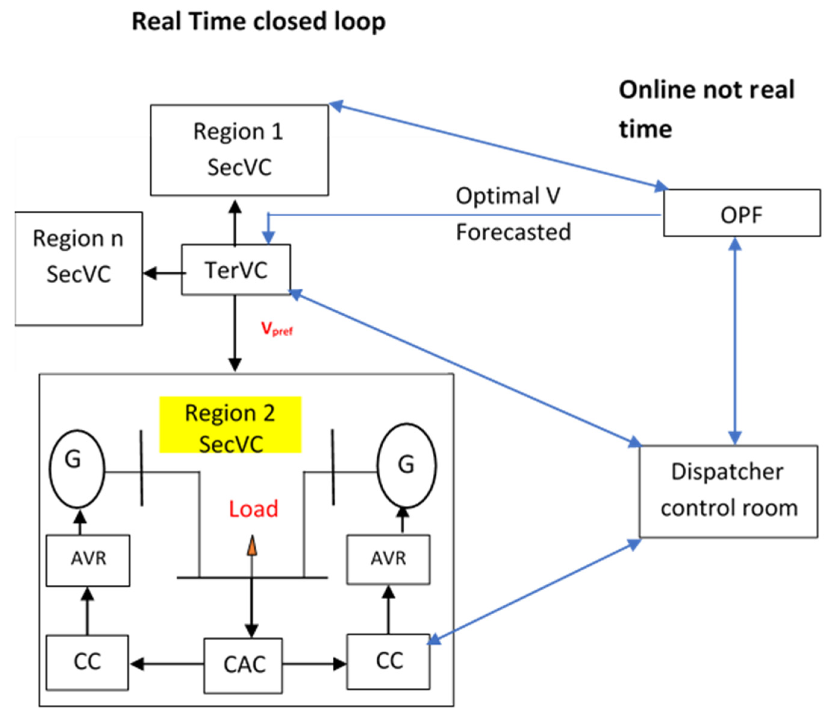
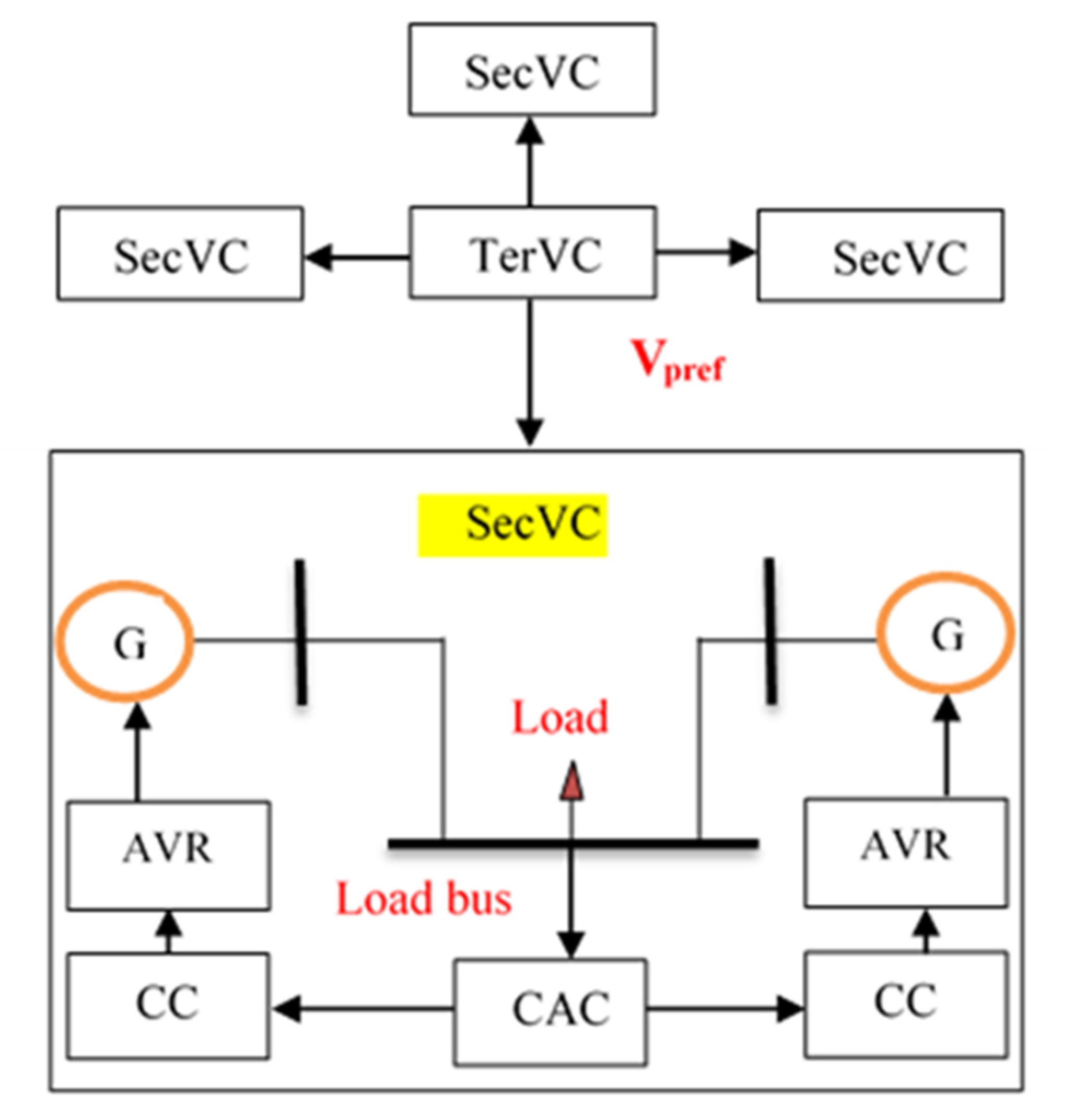
Voltage and reactive power control of a network requires geographical and temporal coordination of many on-field components and control functions achievable by a hierarchical control structure. A real-time and automatic voltage control system can, in fact, be basically structured in three hierarchical levels: primary (component control), secondary (area control) and tertiary (power system control and optimization) levels [3]. Figure 1 provides a main spatial view of the three overlapping hierarchical levels of a voltage and reactive power control system. It also illustrates how the combination is conducted between the TerVC, the load forecasting-based state estimation, in addition to the optimal power flow to achieve a certain objective(s).

The structure of voltage and reactive power control hierarchy of a power system, as shown in Figure 1, consists of:

• The first level is targeting the control of the terminals’ voltage of the generator through an automatic voltage regulator (AVR). This level has the quickest response compared to the other two levels. The control is applied through controlling the field current of the generator.
• The second level targets the cluster control (CC), which controls the reactive power to track the value obtained by the central area control (CAC) at a higher hierarchical level, through an additional signal to the primary voltage control set-point.
• The third level has a slower CAC response. It consists of a few regional voltage regulators (RVRs), if the grid is subdivided into more than one region. For example, the case of a national dispatcher operating on-field through regional dispatchers, which controls the voltage of the pilot nodes by controlling the reactive power of regional generators in the second hierarchical level.

The voltage control hierarchy requires real data measurements for two purposes:

(a)

monitor the changes of the load bus voltage;

(b)

select the optimal sharing of reactive power of each generator to reach optimal operation condition.

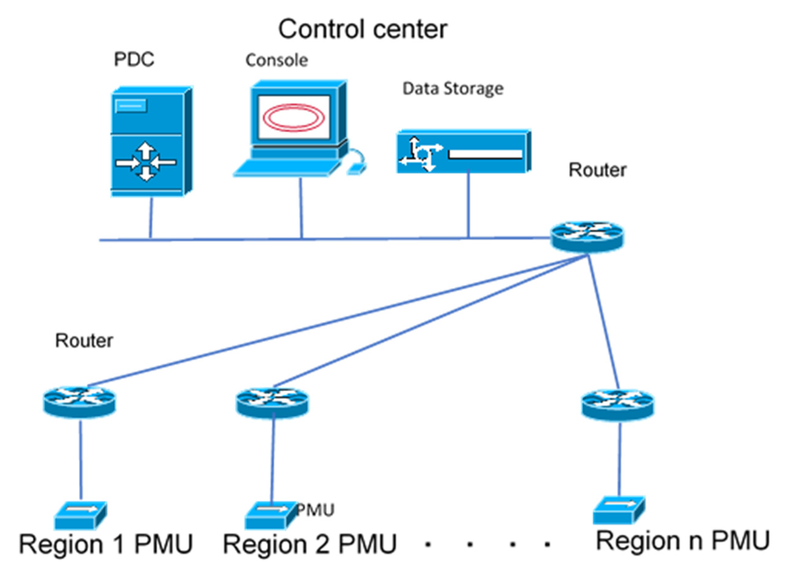
Figure 2 shows the configuration of wide area measurement system to apply three real-time levels of voltage control hierarchy. WAMS-based real-time measurement enables the monitoring of the most sensitive load bus of each region (pilot bus) to apply tertiary and secondary voltage control. One PMU was selected to measure the voltage magnitude of the pilot bus of each region. The complete WAMS configuration is illustrated in Section 8.

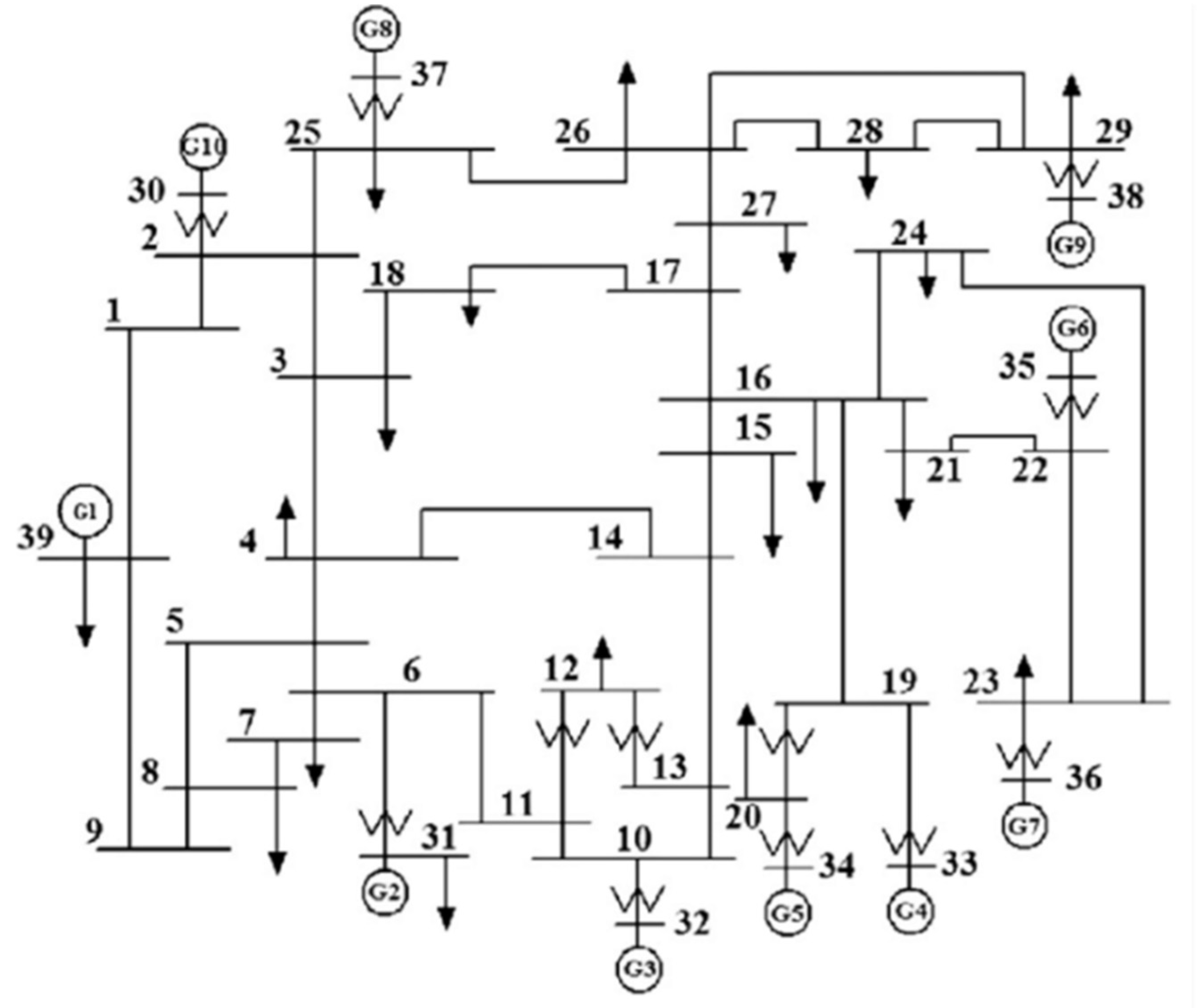
3. IEEE 39 Bus System Description

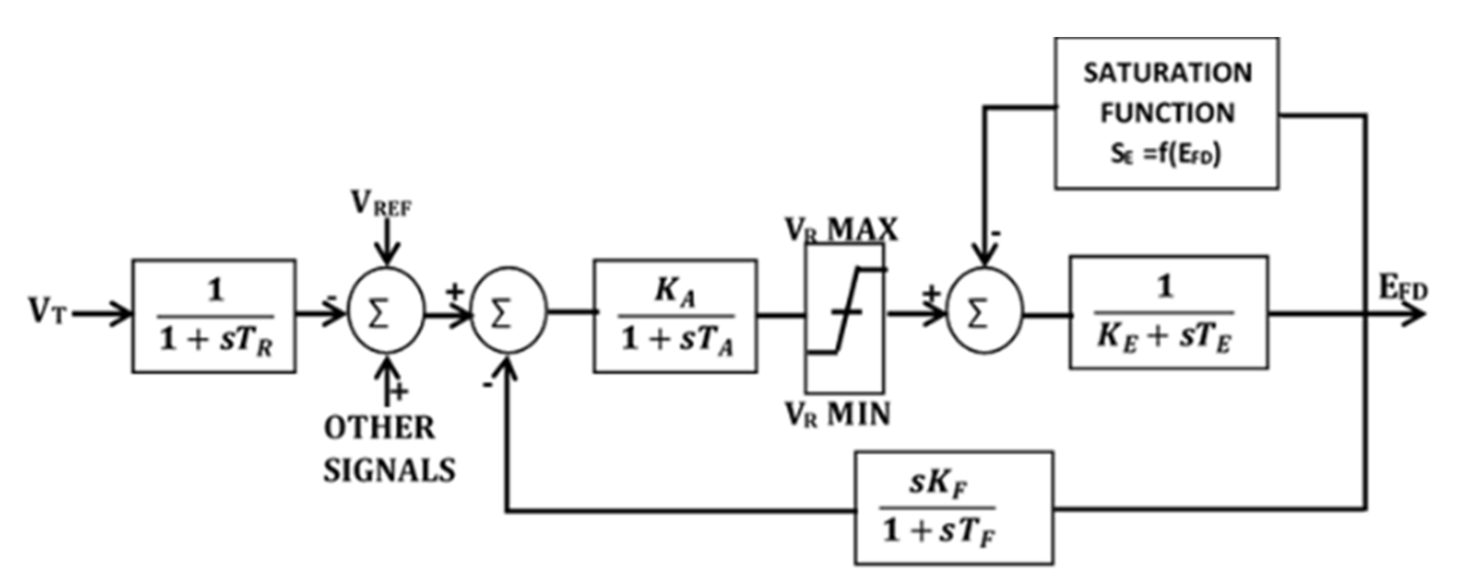
Figure 3 shows the simulated IEEE 39 bus system [21]. The simulated system consists of 39 buses (29 load (PQ) buses and 10 generator (PV) buses), 10 generators and 46 transmission lines. Each generator is equipped with an IEEE Type 1 excitation system (AVR model IEEE T1) as shown in Figure 4 [21], and IEEE standard governor as shown in Figure 5 [22]. In our study, it is assumed that all the generators have the same types of AVRs and governors, but with different parameter values in terms of gains, time constants and limits. The system line and bus data, governor and AVR data are mentioned in Appendix A.

4. Power System Partitioning

In large power systems, to apply SecVC, the grid should be partitioned into regions; then, a pilot bus is selected for each region.

The power system partitioning for secondary voltage control is mainly dependent on two main factors, which are the upgrade of the power system and the dependence of these areas with power system operation condition. Generally, the partitioning aims to avoid the interaction between regions in terms of reactive power exchange and closed loop overlap.

Many researchers proposed different techniques for system partitioning [10], which are:

(a)

partitioning based on geographical regions (applied to real grids);

(b)

partitioning methods based on electrical distance;

(c)

heuristic and meta-heuristic partitioning methods;

(d)

partitioning methods based on graph theory;

(e)

partitioning methods based on learning approach;

(f)

partitioning based on hybrid approach.

The researchers in [10] compared between those techniques on the IEEE 39 bus system and the results indicated that partitioning based on graph theory drives the system to better performance.

The partitioning matrix is the solution of the graph theory method, such that the ith column has the graph buses that belong to the ith partition. This partition matrix minimizes the objective function Equation (1),

$$F={\displaystyle \sum }_{B_i}{\displaystyle \sum }_{B_j}{S}_{ij}$$

(1)

The apparent power between bus number i and bus number j ($S_{ij}$), where i and j range from 1 to 39 in the IEEE 39 bus system, such that i ǂ j; $S_{ij}$ belongs to different regions representing the weights of the lines cut by regions.

The optimization result of the partitioning process is subjected to a condition that each partition should include one generator (reactive power source), at least, to generate or consume reactive power as part of voltage control of the buses in each partition. The graph theory partitioning method is applied to the IEEE 39 bus system and the results show that the system can be partitioned into six regions, as illustrated in

Table 1. Buses in each region (with copyright permission from with copyright permission from [21], IEEE, 2019).

Region ID	Buses in the Region
1	1, 39
2	2, 3, 25, 30, 37
3	4, 5, 7, 8, 9, 6, 31, 11, 10, 32, 13, 12, 14
4	27, 38, 28, 29, 26
5	33, 34, 20, 19, 15, 16, 21, 22, 35, 17, 18
6	23, 24, 36

, as part of the minimization process, which stated in Equation (1).

5. Pilot Bus Selection

To implement secondary voltage control, a linearization is required. Three alternatives can be used to describe the relation between changes of voltages and (active and reactive) power variations as a requirement of linearization, which are [23]:

(1)

Solving power flow based on fast decoupled method, which relates voltage and reactive power variations relation based on sensitivity matrix and is made equal to the negative nodal susceptance matrix of the whole system.

(2)

To consider the active power flows in the electric network, a detailed model was used, but neglects the effect of active power changes on voltage magnitudes. The detailed model is used in this study to linearize the IEEE 39 bus system, and it was also used in [23] to linearize the Egyptian power system.

(3)

The exact model which considers the effect of both active and reactive powers variations on the voltage.

$$\left[\begin{array}{cc}{S}_{GG}& S_{GL}\\ S_{LG}& S_{LL}\end{array}\right]\left[\begin{array}{c}\Delta V_G\\ \Delta V_L\end{array}\right]=\left[\begin{array}{c}\Delta Q_G\\ \Delta Q_L\end{array}\right]$$

(2)

where $\Delta V_G$ is the change of voltage control bus voltage; $\Delta V_L$ is the change of load bus voltage; $\Delta Q_G$ is the change of generated reactive power; while $\Delta Q_L$ is the change of load reactive power, knowing that S_GG, S_GL, S_LG and S_LL, are submatrices that represent the relation between a change of voltage with a change of reactive power.

From Equation (2), it is found that:

$$\Delta V_L=A\Delta Q_L+B\Delta V_G$$

(3)

$A$ in Equation (3) is the inverse of $S_{LL}$ submatrix; while B is a negative multiplication between inverse of $S_{LL}$ submatrix and $S_{LG}$ submatrix.

Since the control should be applied to certain load buses, these are called pilot buses. The control of those pilot buses should keep the voltage stability and performance in the whole system.

$$\Delta V_P=M\Delta V_L$$

(4)

M is a binary matrix (0 or 1) with a size (n_P × n_L) to indicate which load buses are pilot buses; n_P is the number of pilot buses while n_L is the number of load buses in the system.

The pilot buses were selected in each region by calculating the sensitivity matrix of the system and the load bus with the highest sensitivity factor $\partial \mathrm{V}/\partial \mathrm{Q}$ in each region was selected to be a pilot bus [10,11].

Table 2. System pilot buses (with copyright permission from [21], IEEE, 2019).

Region ID	Pilot Bus
1	Bus 1
2	Bus 3
3	Bus 4
4	Bus 27
5	Bus 16
6	Bus 24

illustrates the pilot bus of each region which has the highest $\partial \mathrm{V}/\partial \mathrm{Q}$ among the load buses of the region, because this means that this load bus voltage change is the most sensitive one to the reactive power changes and if it reaches optimal solution; the remaining load buses are optimally operated in terms of voltage magnitude. In fact, theoretically, for each operation condition, the pilot bus of the region may differ; however, to implement SecVC practically, since equipment of measurement and control is required, a one pilot bus is selected based on the $\partial \mathrm{V}/\partial \mathrm{Q}$ of the normal operating conditions.

6. Tertiary Voltage Control

Tertiary voltage control (TerVC) is responsible for changing the setting point of the pilot bus voltages to implement secondary voltage control (SecVC) based on optimal power flow process. Figure 6 shows the applied voltage control hierarchy. The optimal power flow is applied based on the following description:

➢

Objective function which may include one or more of the following: minimization of total active power losses, load shedding, generation cost or maximum reactive power reserve.

➢

Variables: buses voltage (magnitude and angle) and generators’ active and reactive power.

➢

Constraints: The optimization process is subjected to the following conditions:

-

power flow equations:

$${\displaystyle \sum }PG-{\displaystyle \sum }PD-{\displaystyle \sum }PLoss=0$$

(5)

$${\displaystyle \sum }QG-{\displaystyle \sum }QD-{\displaystyle \sum }QLoss=0$$

(6)

-

generating limits for each generator:

$$P{G}_{min}\le PG\le P{G}_{max}$$

(7)

$$Q{G}_{min}\le QG\le Q{G}_{max}$$

(8)

-

bus voltage magnitude level limits:

$$V{b}_{min}\le Vb\le V{b}_{max}$$

(9)

-

each line loading thermal limit:

$$Pline\le Plin{e}_{max}$$

(10)

The optimal power flow objective may include multi-objective; In this paper, the objective function was selected to minimize the total active power losses. In Equation (9), the acceptable voltage values bounds differ from an operating scenario to another. The voltage bounds at normal operating condition ranges between 95% and 105% of the rated bus voltage magnitude, while during contingency (generator outage or line outage), the limits should be 90% and 110% of the nominal bus voltage magnitude, respectively.

7. Secondary Voltage Control

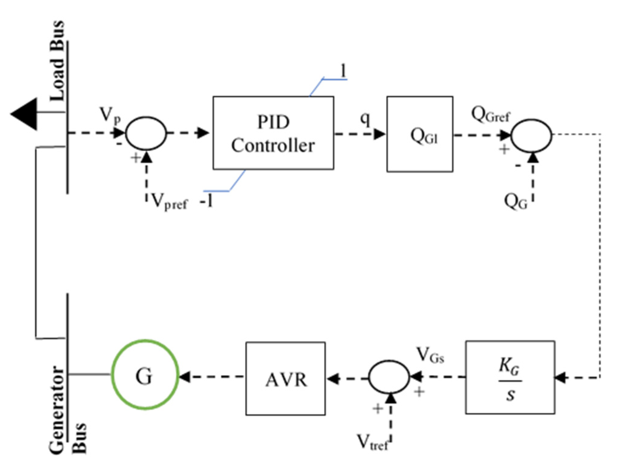
As illustrated in [5], the control strategy in Figure 6 and Figure 7 achieves secondary voltage control. The strategy was simulated in MATLAB/SIMULINK 2017a and the output of SecVC control strategy is an additional signal to the AVR reference.

The following equations describe the control strategy:

i.

Central area control (CAC) equations:

$$V_{pref}-V_p=\Delta V_p$$

(11)

$$q={\left|K_p\Delta V_p+K_I\underset{0}{\overset{t}{{\displaystyle \int }}}\Delta V_{p}dt+K_D\frac{d\Delta V_p}{dt}\right|}_{-1}^{+1}$$

(12)

ii.

Unit cluster control (CC) equations:

$$Q_{ref}=q\ast Q_{Gl}$$

(13)

$$V_{GS}=\frac{K_G}{s}\left(Q_{ref}-Q_G\right),K_G=\frac{X_{TG}+X_{eq}}{T_G}$$

(14)

where V_pref is the pilot bus reference voltage calculated from the tertiary voltage control; $V_p$ is the pilot bus actual voltage; $\Delta V_p$ is the pilot bus voltage error; $q$ represents the amount of reactive power required in percentage to track the pilot bus voltage ranging between −100% and 100%. The term q from the control point of view is the secondary voltage PID control action. $Q_{Gl}$ is the reactive power limit known from generator capability curve; $V_{GS}$ is the additional signal to the AVR reference. The regulator integral gain, K_G, is calculated from the sensitivity matrix; $X_{TG}$ is the generator transformer impedance; $X_{eq}$ is the line impedance; the time constant $T_G$ is set to be 5 s [2,4].

8. WAMS Configuration in IEEE 39-Bus System

The WAMS consists of the following components as illustrated in Figure 2:

(1)

PMUs;

(2)

phasor data concentrator (PDC);

(3)

communication network;

(4)

operator console;

(5)

data storage.

Since PMUs are expensive, the installation of a PMU in each busbar is far from being applicable. To apply secondary voltage control only in a multi-region power system, one PMU in each region is sufficient. The PMU is installed in the pilot bus of the region. After selection of the pilot bus of each region, the optimal placement of the PMUs in the IEEE 39 bus system is at buses 1, 3, 4, 16, 24 and 27. This selection criterion will reduce the price of WAMS configuration by 57%, if the method applied in [24] is used. In [23], the authors minimized the number of PMUs for each region, then selected the optimal placement of PDC to apply secondary voltage control to the Egyptian grid. According to [23], for the IEEE 39 bus system to fully reach the measurement of each busbar, 14 PMUs are required.

9. Secondary Voltage Controllers Design

Since one of the main features of smart grid is self-healing, which requires a real-time optimal control at different power grid operating conditions, artificial intelligence is the key to implement this feature. In this paper, the secondary voltage control was applied by a genetic PID controller, instead of the conventional one, the parameters of which were selected through mathematical local minimization or trial and error.

9.1. Genetic Secondary PID Controller

The design of PID controllers will be performed for each operation condition separately, using the genetic algorithm (GA) toolbox in MATLAB to enable the pilot bus to reach its optimal value at this condition. The optimization problem is described as follows:

Objective function: minimizing integration of square error ($\Delta {\mathrm{V}}_{\mathrm{p}}$)

$$\min {\int }_0^{\mathrm{t}}{\left(\Delta {\mathrm{V}}_{\mathrm{p}}\right)}^2\mathrm{dt}$$

(15)

Variables: PID controller parameters ($K_p$, $K_I$ and $K_D$).

Constraints: q limits (±100%) and generated reactive power limits.

The GA is an iterative optimization technique, working with a number of candidate solutions (known as a population). In many engineering problems, the initial start of GA begins its search with a random population of solutions [25]. GA is available in MATLAB and the parameters are set such that the population type is double vector while the population size of 20. The crossover fraction is set to be 0.8, while the elite count reproduction is 2. To reduce the possibility of reaching local minima, instead of global one, mutation rate is increased and the optimization process is repeated using the optimal solution as the initial one [26].

9.2. Neural Network Based on Genetic Secondary PID Controller

An artificial neural network (ANN) is a group of neurons in the form of simple processing units that are linked to each other to obtain a behaviour that is like human behaviour when solving an engineering problem [27].

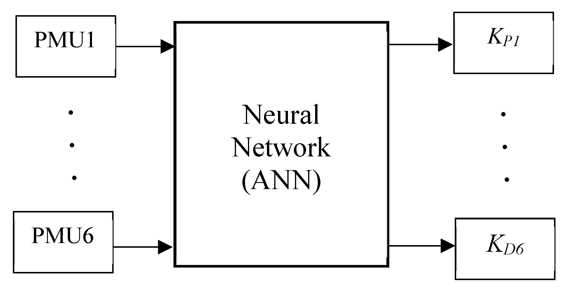
Many research papers have presented studies in voltage stability and control based on ANN. In [28], the study presented an application of ANN for monitoring power system voltage stability, while in [29], the study proposed and used ANN to help the dispatcher reach an optimal decision during contingencies. ANN is used in the static voltage stability to instantaneously map a contingency to a set of controllers where the types, locations and amount of switching can be induced. In this study, a design for the secondary voltage PID controller of each region is proposed. The system is then assumed to be subjected to different contingencies and disturbances to examine the controller’s performance. An artificial intelligence facility (ANN) is used to select the optimal parameters of the secondary voltage PID controllers at each operation condition. The PMU readings of the voltage magnitudes of the pilot buses will be the input to the neural network, which will decide the optimal values of the PID designed for the specific contingencies, as shown in Figure 8. The ANN used in this work has 6 inputs, due to the presence of 6 PMUs—so18 outputs (which are the secondary PID controllers’ parameters, since there are 6 partitions, so there are 6 controllers, and each one has 3 parameters, meaning a total 18 outputs)—and the ANN includes a 10-neurons hidden network. The network is designed and trained using the Levenberg–Marquardt backpropagation method [2,30].

10. Simulation Results

In this section, the power analysis was calculated through the DIgSILENT software application, while the controllers were designed in MATLAB/Simulink; the voltage and reactive power responses were extracted from MATLAB.

10.1. Pilot Bus Selection Results

To select the pilot buses, a sensitivity analysis calculation took place in DIgSILENT in the base case, and the results are shown in

Table 3. IEEE 39 bus system sensitivity analysis.

Bus Number	$\partial \mathbf{V}/\partial \mathbf{Q}\mathbf{Sensitivity}$	Bus Type
Bus 01	0.00007019	Load
Bus 02	0.00006587	Load
Bus 03	0.0001086	Load
Bus 04	0.00012131	Load
Bus 05	0.00010647	Load
Bus 06	0.00009825	Load
Bus 07	0.00011146	Load
Bus 08	0.00011652	Load
Bus 09	0.00011003	Load
Bus 10	0.00010175	Load
Bus 11	0.00011061	Load
Bus 12	0.00012945	Load
Bus 13	0.00011819	Load
Bus 14	0.00012329	Load
Bus 15	0.00013818	Load
Bus 16	0.00018721	Load
Bus 17	0.00011178	Load
Bus 18	0.00013338	Load
Bus 19	0.00008075	Load
Bus 20	0.00010599	Load
Bus 21	0.00012905	Load
Bus 22	0.00008155	Load
Bus 23	0.00010072	Load
Bus 24	0.00012289	Load
Bus 25	0.00008623	Load
Bus 26	0.00015584	Load
Bus 27	0.00017512	Load
Bus 28	0.00011630	Load
Bus 29	0.00012676	Load
Bus 30	0	Generator
Bus 31	0	Generator
Bus 32	0	Generator
Bus 33	0	Generator
Bus 34	0	Generator
Bus 35	0	Generator
Bus 36	0	Generator
Bus 37	0	Generator
Bus 38	0	Generator
Bus 39	0	Generator

; the highest load bus value in each area is selected to be the pilot bus of this region, as mentioned in Table 2.

10.2. Tertiary and Secondary Voltage Control Results

10.2.1. Base Case (B.C.): Normal Operating Conditions

During the normal operating condition (base case), a minimization of total active power losses is performed considering the constraints of Equations (5)–(10). The results are listed in

Table 4. Optimal power flow results at base case, case 1, case 2, case 3 and case 4.

Bus Number	Optimal Voltage
	Base Case	Case 1	Case 2	Case 3	Case 4
Bus 01	1.0046	1.0038	1.0050	1.0040	1.0040
Bus 02	1.0187	1.0187	1.0194	1.0009	1.0004
Bus 03	1.0025	1.0256	1.0050	1.0500	1.0250
Bus 04	0.9645	0.9645	0.96395	0.9640	0.9640
Bus 05	0.9642	0.9642	0.9642	0.9641	0.9641
Bus 06	0.9673	0.9673	0.9673	0.9673	0.9673
Bus 07	0.9589	0.9589	0.9589	0.9589	0.9589
Bus 08	0.9591	0.9591	0.9591	0.9591	0.9591
Bus 09	1.0194	1.0188	1.0188	1.0188	1.0188
Bus 10	0.9552	0.9594	0.9593	0.9594	0.9594
Bus 11	0.9609	0.9609	0.9607	0.9609	0.9609
Bus 12	0.9444	0.9444	0.9443	0.9444	0.9444
Bus 13	0.9577	0.9577	0.9577	0.9577	0.9577
Bus 14	0.9579	0.9579	0.9579	0.9579	0.9579
Bus 15	0.9670	0.9670	0.9670	0.9670	0.9670
Bus 16	0.9910	0.9600	0.9946	0.9948	0.9948
Bus 17	0.9748	0.9748	0.9938	0.9938	0.9938
Bus 18	0.9778	0.9778	0.9888	0.9888	0.9888
Bus 19	1.0321	1.0321	1.0321	1.0321	1.0321
Bus 20	0.9804	0.9804	0.9805	0.9804	0.9804
Bus 21	1.0002	1.0002	1.0003	1.0002	1.0002
Bus 22	1.0307	1.0307	1.0307	1.0307	1.0307
Bus 23	1.0245	1.0245	1.0245	1.0245	1.0245
Bus 24	0.985	1.0002	0.9804	1.0001	1.0001
Bus 25	1.0409	1.0409	1.0408	1.0014	1.0011
Bus 26	1.0226	1.0226	1.0226	1.0226	1.0226
Bus 27	1.0024	1.0024	1.0022	1.0024	1.0024
Bus 28	1.0285	1.0285	1.0285	1.0285	1.0285
Bus 29	1.0335	1.0335	1.0335	1.0335	1.0335
Bus 30	1.0475	1.0475	1.0475	1.0475	1.0475
Bus 31	0.9823	0.9823	0.9820	0.9825	0.9825
Bus 32	1.0008	1.0008	0.9896	0.9896	0.9896
Bus 33	0.9972	0.9972	0.9972	0.9972	0.9972
Bus 34	1.0123	1.0123	1.0123	1.0123	1.0123
Bus 35	1.0493	1.0493	1.0493	1.0493	1.0493
Bus 36	1.0635	1.0635	1.0635	1.0635	1.0635
Bus 37	1.0278	1.0278	1.0278	1.0278	1.0278
Bus 38	1.0265	1.0265	1.0265	1.0265	1.0265
Bus 39	1.0404	1.0404	1.0404	1.0404	1.0404

. To achieve these optimal voltages, SecVC is applied. The IEEE 39 bus system includes six regions with a SecVC applied to the pilot bus of each region. The reactive power of the generator of the region supports the pilot bus voltage to track optimal value, as shown in

Table 5. Pilot buses supportive generators (with copyright permission from [21], IEEE, 2019).

Pilot Bus	Supportive Generator	Pilot Bus	Supportive Generator
Bus 01	Generator at Bus 39	Bus 16	Generator at Bus 35
Bus 03	Generator at Bus 37	Bus 24	Generator at Bus 36
Bus 04	Generator at Bus 31	Bus 27	Generator at Bus 38

. The genetic PID secondary controller is used for each region to automatically inject or absorb reactive power of each region. The parameters of each PID controller at the normal operating condition (Base Case (B.C.) PID) are calculated to achieve Equation (15) and shown in

Table 6. Genetic proportional integral derivative (PID) parameters of each control region at base case (with copyright permission from [21], IEEE, 2019).

Region Number	Kp	KI	KD
1	1.23	0.34	0.14
2	5.47	2.94	2.33
3	2.18	0.96	0.76
4	4.56	1.58	0.97
5	1.78	1.26	1.07
6	2.57	1.47	0.46

. The rest of the parameters of the SecVC are derived from the IEEE 39 bus data.

10.2.2. Case 1: Generator Contingency in Region 5

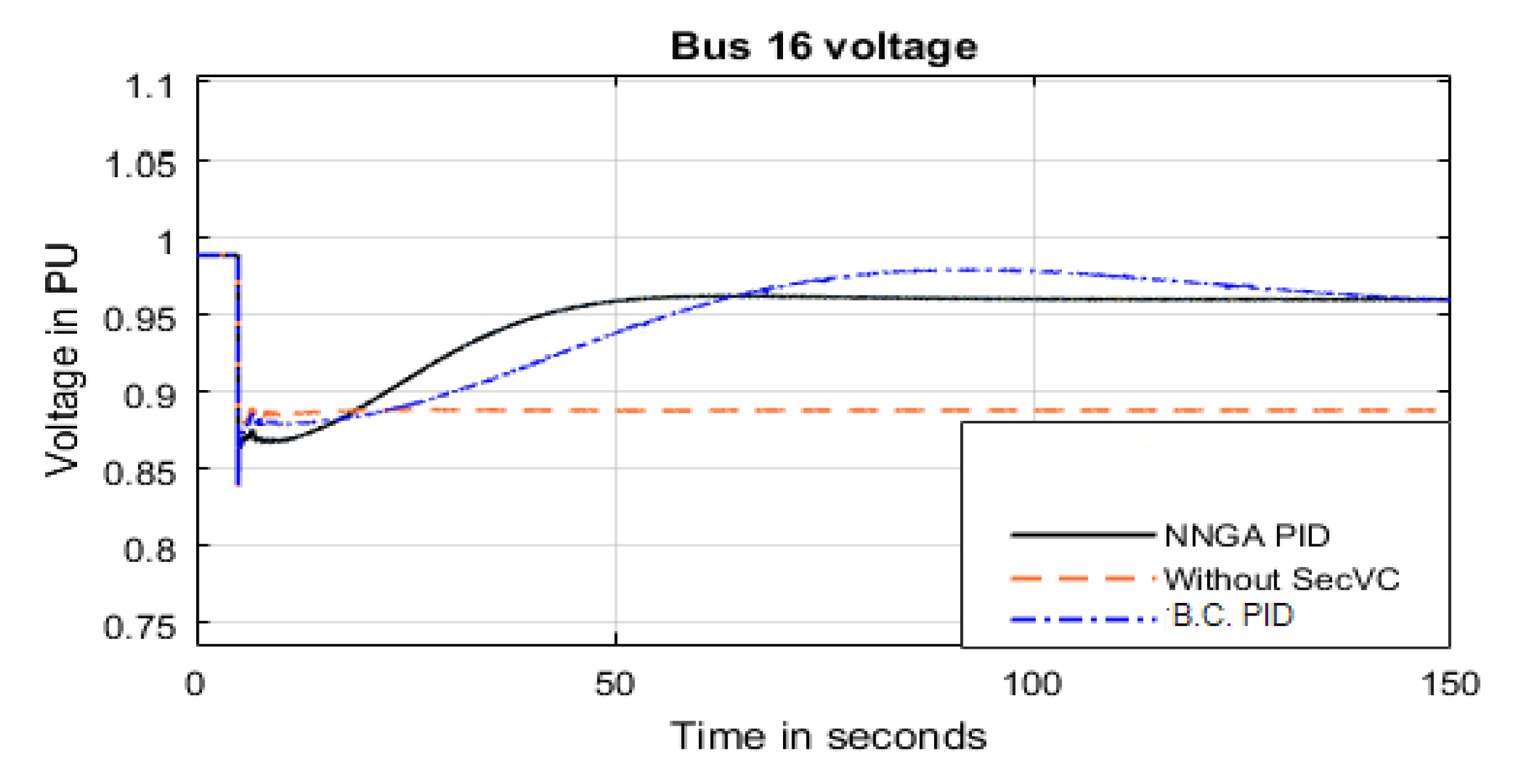
In this case, a generator outage occurred in bus 33 generator. After simulating the mentioned generator outage, an optimal power flow calculation was performed; the results are listed in Table 4. The TerVC results show that most of the change occurred to Bus 16, the pilot bus of the fifth partition voltage, unlike the other pilot buses, which changed only slightly, by 0.07% or less. The results show that, without SecVC, bus 16 voltage magnitude reduced to 0.88 pu, which means it was out of the acceptable range, which is 10% below the nominal voltage.

Table 7. Genetic PID parameters of each control region at case 1.

Region Number	Kp	KI	KD
1	1.23	0.34	0.14
2	5.47	2.94	2.33
3	2.18	0.96	0.76
4	4.56	1.58	0.97
5	4.21	2.51	0.74
6	2.57	1.47	0.46

shows optimal PID parameters at this operating condition calculated using GA and stored in the neural network. Figure 9 shows that, by applying SecVC using genetic PID controllers, pilot bus voltage reached the optimal value to achieve minimum power losses at this case, which is 0.96 pu. Figure 10 shows the reactive power support to raise the voltage of the pilot bus to the optimal value. The results also show that the system performance using the NNGA PID controllers (case 1 PIDs) was better than that of B.C. PID controllers, which were designed in the normal operating condition.

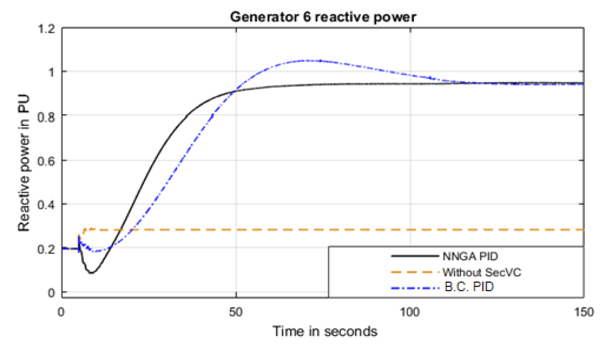
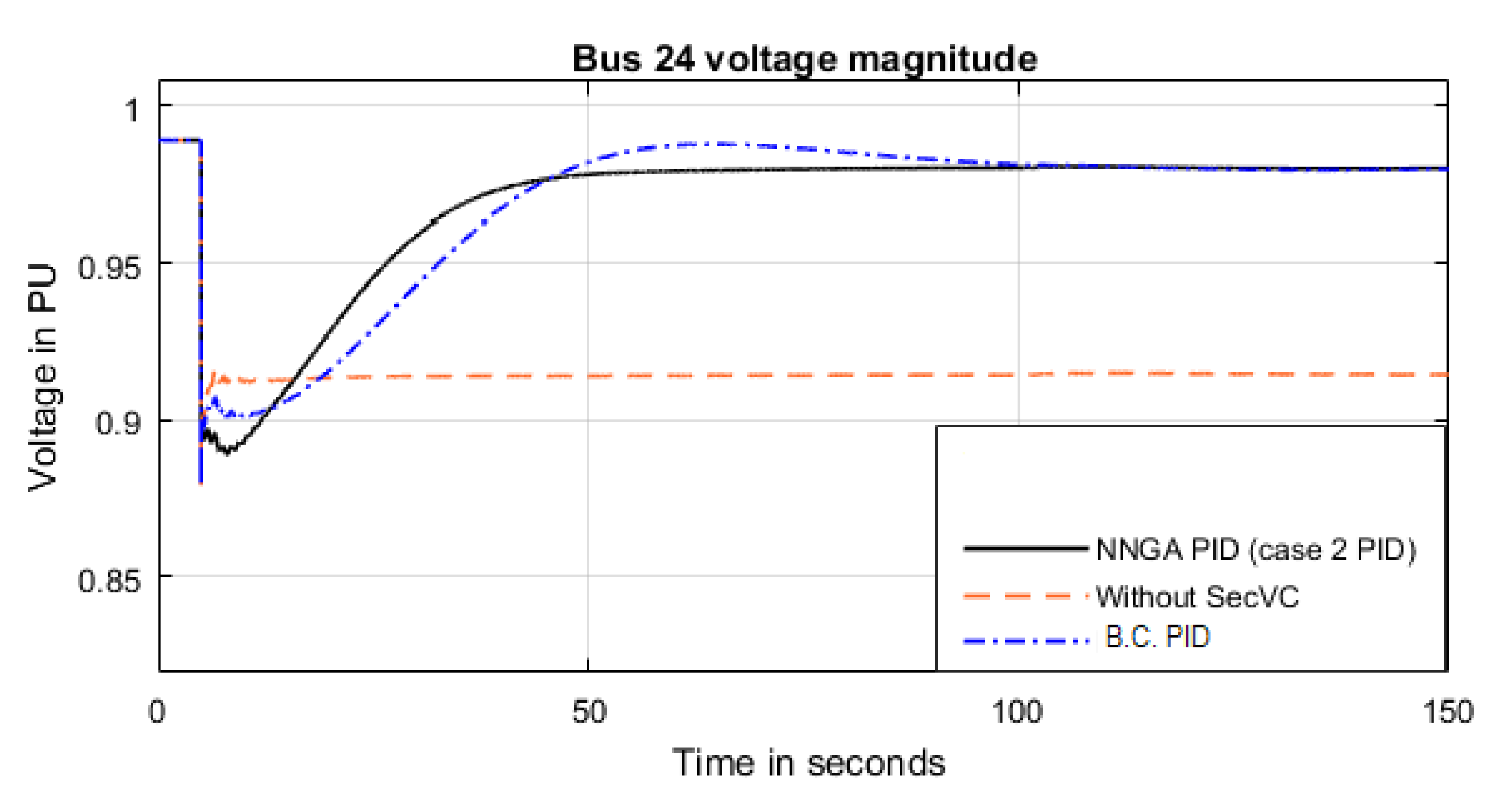
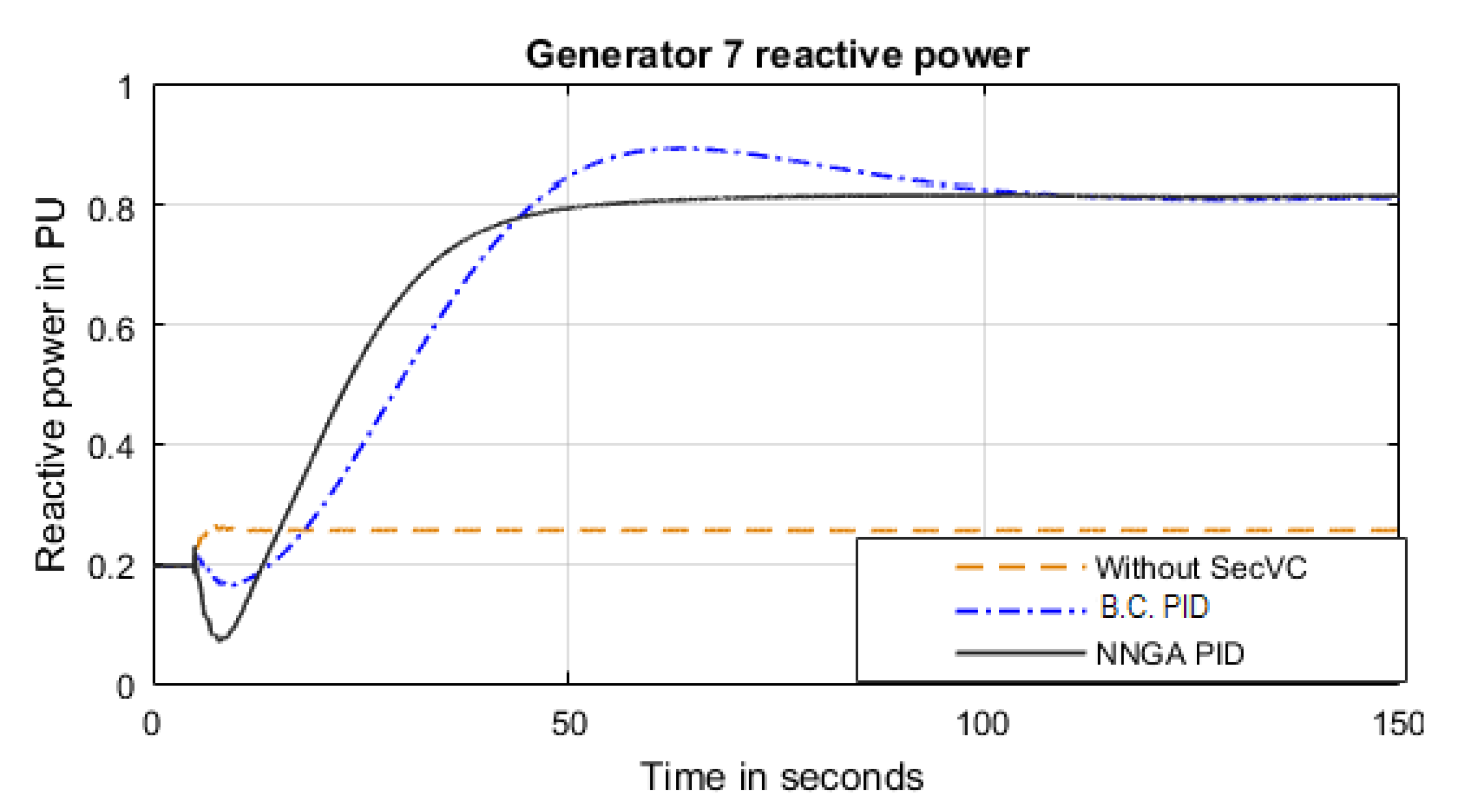
10.2.3. Case 2: 50% of Generating System Outage in Region 6

In this case, it was assumed that 50% of the generation at bus 36 goes out of service after 5 s. In bus 24, the pilot bus of sixth region, the voltage reduced, due to this contingency, to 0.91 pu, which led to a weak voltage profile. The optimal power flow calculations were performed to minimize the total active power losses at this case; the output results listed in Table 4 indicate that the optimal value of bus 24 is 0.98 pu. The genetic PID controllers that were designed for the base case were used to enable us to reach the optimal value of bus 24. Furthermore, the genetic PID controller was redesigned again at this condition and stored in the neural network. The optimal PID parameters of each region at this condition are presented in

Table 8. Genetic PID parameters of each control region at case 2.

Region Number	Kp	KI	KD
1	1.23	0.34	0.14
2	2.2	1.51	0.58
3	1.82	0.96	0.74
4	1.45	0.27	0.07
5	1.48	1.06	0.98
6	3.58	2.19	0.89

. The results in Figure 11 and Figure 12 show that NNGA PID controllers reached the desired value, with a performance better than that of base case genetic PID. The reason for that is the fact that the system is highly non-linear and, in each disturbance, the power system configuration changes; therefore, it requires adaptive changes of PID parameters. This highlights the robustness of NNGA PID, rather than of B.C. GA.

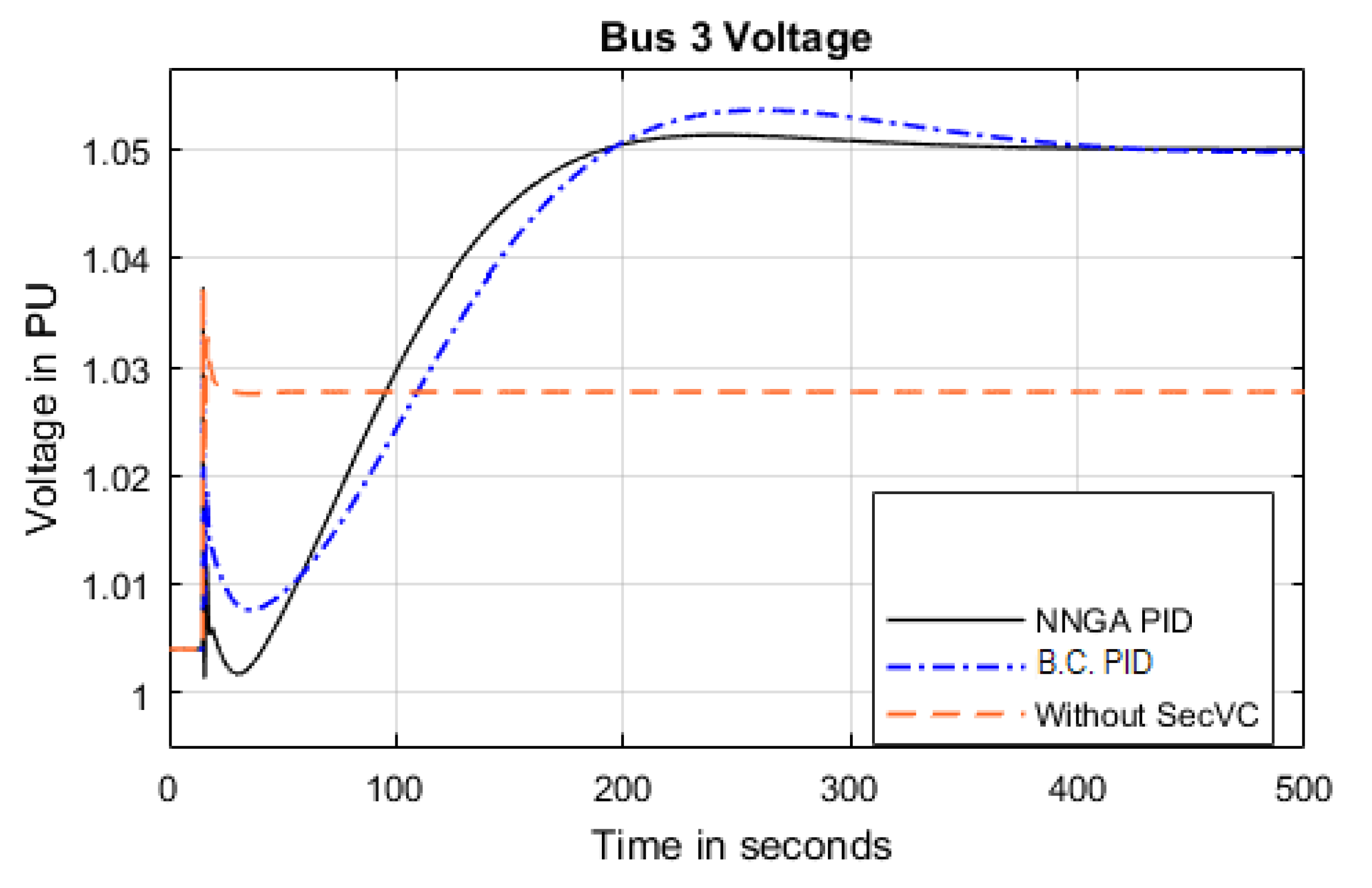
10.2.4. Case 3: Line Contingency

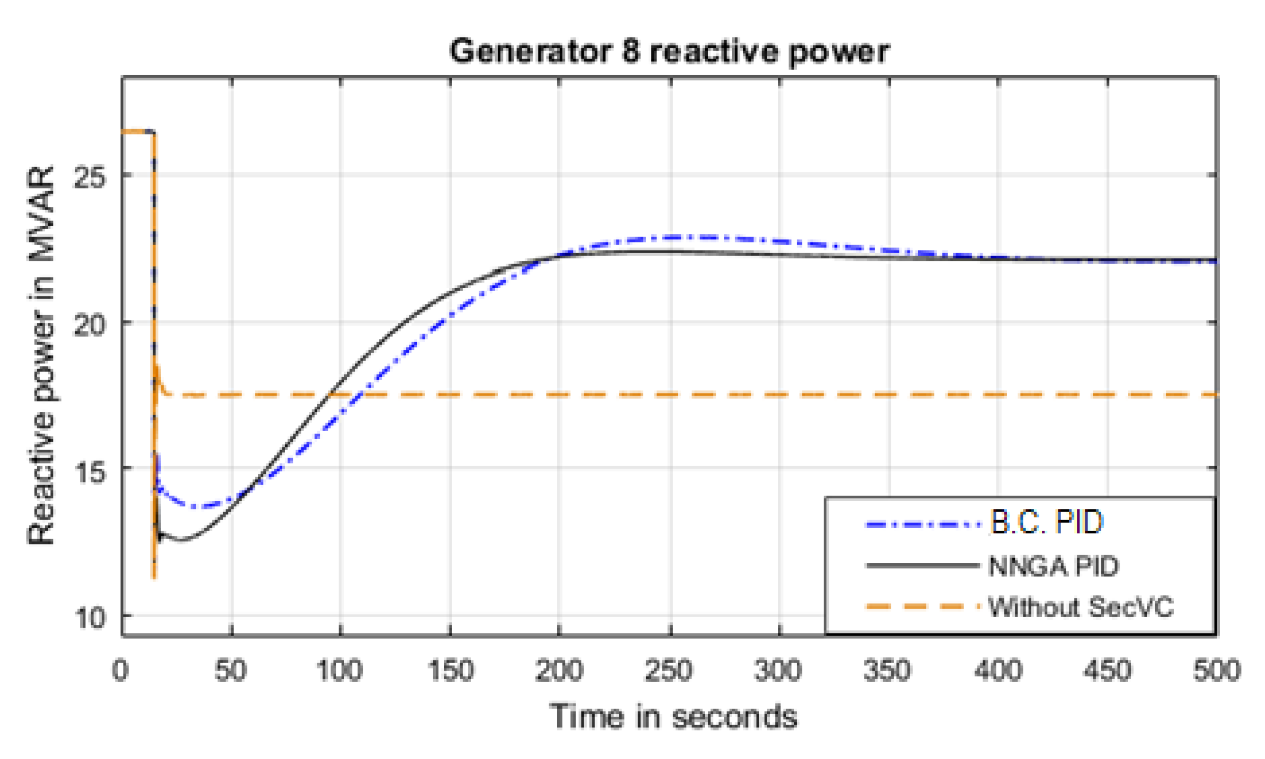
In this case, the line connecting between bus 3 and bus 4 went out of service after 15 s from the beginning of the simulation. Optimal power flow calculations to achieve minimum losses were performed at this case; Table 4 shows the optimization results. The results show that, for bus 3, the pilot bus of region 2, optimal voltage magnitude reached 1.05 PU, but at the same time, the voltage deviation of the other load buses in the same region (bus 2 and bus 25) decreased and they have a voltage magnitude near their rated values. The results show that the pilot bus voltage in region two was affected, at this contingency, by 4.5%, unlike the other regions, which were almost constant. The previously designed genetic algorithm PID controllers, that were designed in base case, were used to enable reaching optimal value of bus 3. Furthermore, the genetic PID controller was redesigned again for this case and stored in ANN, based on what if analysis; the PID parameters of each region is presented in

Table 9. Genetic PID parameters of each control region at case 3.

Region Number	Kp	KI	KD
1	1.23	0.85	0.47
2	5.47	2.94	2.33
3	2.18	0.96	0.76
4	1.45	0.27	0.07
5	1.78	1.26	1.07
6	2.57	1.47	0.46

. The results in Figure 13 and Figure 14 show that case 3 genetic PID (NNGA PID) reached the desired value, with a performance better than that of B.C. genetic PID, in terms of maximum overshoot and settling time. This result ensures that NNGA PID controllers are more robust than that of B.C. GA PID controllers.

10.2.5. Case 4: Line Contingency Followed by Load Increase

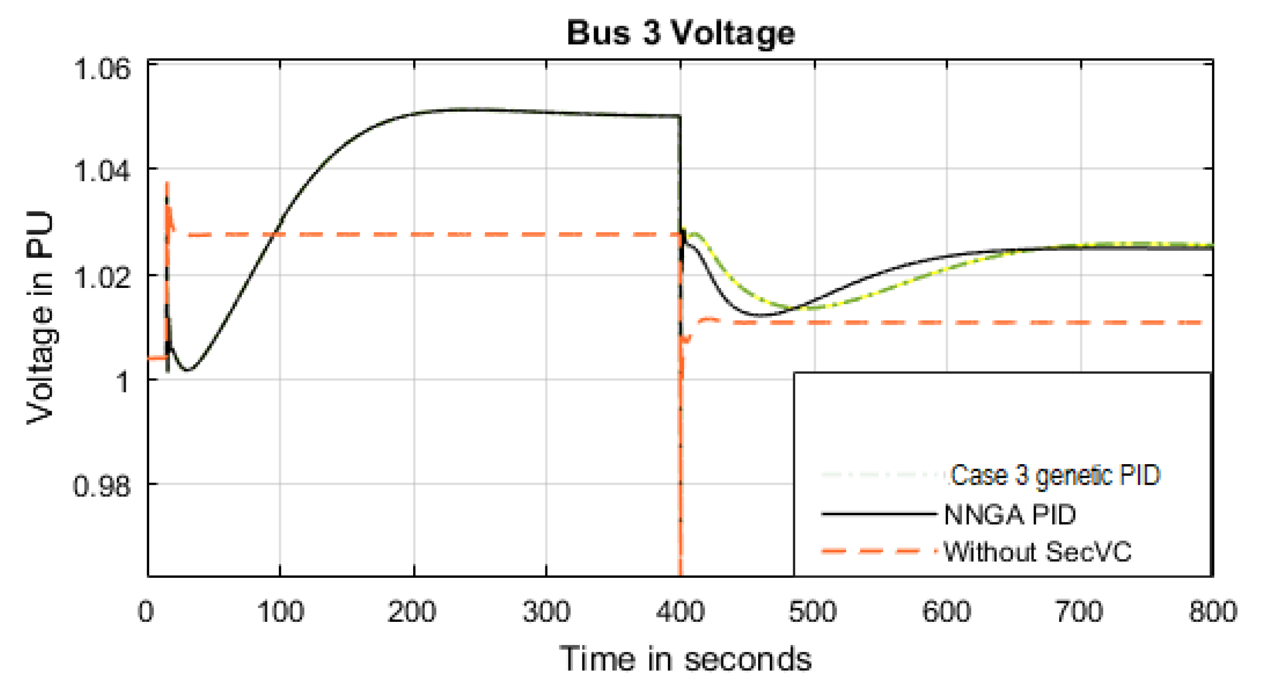
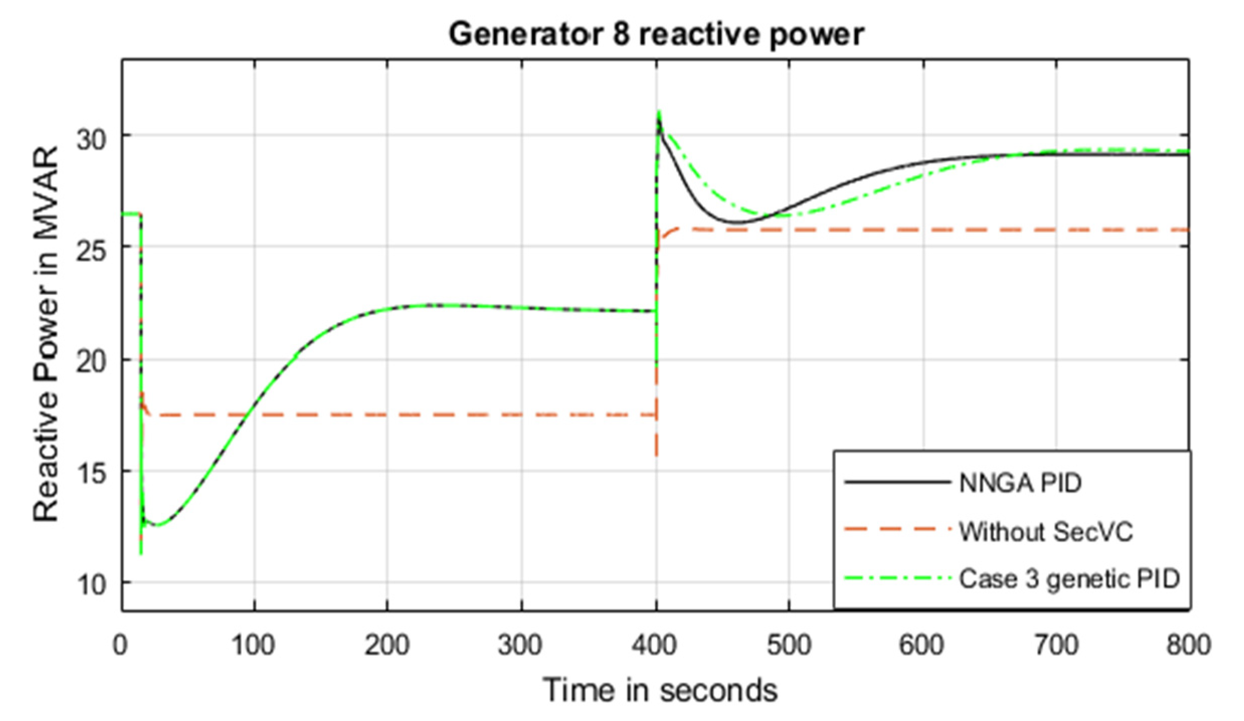
In this case, a 25% load increase in bus 3 event was simulated to occur after the line outage event in case 3 by 400 s. After simulating both events in the steady state, an optimal power flow was calculated to achieve minimum power loss; Table 4 shows the optimization results. The results show that, after the two events, the optimal voltage of bus 3 was 1.025 PU; at the same time, the voltage deviation of the other load buses in this region was less than before. The results show that bus 3 voltage was changed by 2.1% from the normal case after the two events, while they also show that the other pilot buses remain at a steady state or slightly changed by 0.04% or even less.

To achieve the optimal voltages in Table 4, secondary voltage control was applied. Genetic algorithm PID secondary controllers, used in case 3, were also applied in this case. Furthermore, a redesign of GA PID was made for this case after the two events and stored in the ANN. The optimal values of GA PID parameters at case 4 (after simulating the two events) are listed in

Table 10. Genetic PID parameters of each control region at case 4.

Region Number	Kp	KI	KD
1	1.23	0.85	0.47
2	3.14	1.29	1.06
3	2.18	0.96	0.76
4	1.45	0.27	0.07
5	1.78	1.26	1.07
6	2.57	1.47	0.46

; Figure 15 and Figure 16 show that NNGA PID controllers had better performance than case 3 GA PID controllers, in terms of settling time and maximum overshoot after the occurrence of the load increase event. The NNGA had better performance than that of GA after the load increase because the NNGA, through the readings of the PMUs, detected the load increase scenario after the line outage and changed the parameters of the PID to the optimal one at this operating condition.

Table 11. Comparison between pilot bus voltage performance using genetic algorithm (GA) and NNGA.

Cas	Maximum Overshoot in %		Settling Time in Seconds
	GA	NNGA	GA	NNGA
1	2.60	0.52	140	70
2	1.18	0	100	50
3	0.49	0.10	390	320
4	0	0	700	600

and

Table 12. Comparison between supportive generator reactive power performance using GA and NNGA.

Case	Maximum Overshoot in %		Settling Time in Seconds
	GA	NNGA	GA	NNGA
1	8.25	0	110	50
2	20	0	100	50
3	4.5	0	370	200
4	0	0	650	600

illustrate the difference between GA and NNGA for pilot bus voltage and supportive generator reactive power, in terms of maximum overshoot and settling time. The results show better performance from NNGA in all case studies. The results supported the main findings of the paper that for optimal operation, PID parameters change at each operation condition due to the change of the system configuration.

Table 13. Comparison between system with and without secondary voltage control (SecVC).

Case	Losses in MW		Voltage Index
	With SecVC	Without SecVC	With SecVC	Without SecVC
B.C.	53.23	56.21	0.023	0.031
1	78.43	89.10	0.027	0.084
2	68.37	74.54	0.024	0.076
3	49.21	64.21	0.033	0.042
4	51.52	64.86	0.026	0.039

shows the difference between system with SecVC and system without SecVC in terms of voltage index (X_rms) based on Equation (16) and power losses. The results investigated that the system performance is improved in terms of voltage deviation index and total power losses after applying TerVC and SecVC.

$$X_{rms}=\sqrt{\frac{1}{n_L}{\sum }_{i=1}^{n_L}{\left(V_{in}-V_i\right)}^2}$$

(16)

where $n_L$ is the number of load buses in the power system, which is equal to 29 buses in the IEEE 39 bus system. $V_{in}$ is the nominal voltage of the load bus and $V_i$ is the actual load bus voltage. Lower voltage index means better voltage profile [16,30].

11. Conclusions

The paper investigated the application of secondary voltage control on the IEEE 39 bus system as a multi-region power system based on optimal power flow, wide area measurement system and system partitioning. The results proved the ability of the intelligent secondary PID controller to achieve optimal values at different operating conditions. The results also show that NNGA PID controllers can reach voltage optimal values in all conditions, with a performance better than that of GA PID controllers, which requires parameter design for each disturbance, due to the change of system configuration. The study also proved the effectiveness of system partitioning and pilot bus selection methods in the IEEE 39 bus system, as all the load busbars in the system achieved the optimal values. The results proved that generators of the grid might support load buses without adding extra reactive power sources to the system.

References

- Li, F.; Qiao, W.; Sun, H.; Wan, H.; Wang, J.; Xia, Y.; Xu, Z.; Zhang, P. Smart transmission grid: Vision and framework. IEEE Trans. Smart Grid 2010, 1, 168–176. [Google Scholar] [CrossRef]
- Abdalla, O.H.; Ghany, A.M.A.; Fayek, H.H. Coordinated PID secondary voltage control of a power system based on genetic algorithm. In Proceedings of the 2016 Eighteenth International Middle East Power Systems Conference (MEPCON), Cairo, Egypt, 27–29 December 2016; pp. 214–219. [Google Scholar]
- Corsi, S. Voltage Control and Protection in Electrical Power Systems: From System Components to Wide-Area Control; Springer: New York, NY, USA, 2015. [Google Scholar]
- Corsi, S.; Pozzi, M.; Sabelli, C.; Serrani, A. The coordinated automatic voltage control of the Italian transmission grid—Part I: Reasons of the choice and overview of the consolidated hierarchical system. IEEE Trans Power Syst. 2004, 19, 1723–1732. [Google Scholar] [CrossRef]
- Hu, B.; Cañizares, C.A.; Liu, M. Secondary and Tertiary Voltage Regulation based on optimal power flows. In Proceedings of the 2010 IREP Symposium Bulk Power System Dynamics and Control–VIII (IREP), Rio de Janeiro, Brazil, 1–6 August 2010; pp. 1–6. [Google Scholar]
- Guo, Q.; Sun, H.; Zhang, M.; Tong, J.; Zhang, B.; Wang, B. Optimal voltage control of PJM smart transmission grid: Study implementation and evaluation. IEEE Trans. Smart Grid 2013, 4, 1665–1674. [Google Scholar]
- Paul, P.; Leost, J.Y.; Tesseron, J.M. Survey of the secondary voltage control in france: Present realization and investigations. IEEE Trans. Power Syst. 1987, 2, 505–511. [Google Scholar] [CrossRef]
- Arcidiacono, V.; Corsi, S.; Natale, A.; Raffaelli, C.; Menditto, V. New Developments in the Application of ENEL Transmission System Voltage and Reactive Power Automatic Control; CIGRE: Rome, Italy, 1990. [Google Scholar]
- Taranto, G.N.; Martins, N.; Falcao, D.M.; Martins, A.C.B.; Santos, M.G. Benefits of Supplying Secondary Voltage Control Schemes to the Brazilian System. In Proceedings of the IEEE PES Winter Meeting, Singapore, 23–27 January 2000; pp. 937–942. [Google Scholar]
- Alvarez, R.; Mazo, E.H.L.; Oviedo, J.E. Evaluation of power system partitioning methods for secondary voltage regulation application. In Proceedings of the 2017 IEEE 3rd Colombian Conference on Automatic Control (CCAC), Cartagena, Colombia, 18–20 October 2017; pp. 1–6. [Google Scholar]
- Conejo, A.; Gbmez, T.; de la Fuente, J.I. Pilot-bus selection for secondary voltage control. Eur. Trans. Electr. Power 1993, 3, 359–366. [Google Scholar] [CrossRef]
- Daher, N.A.; Mougharbel, I.; Saad, M.; Kanaan, H.Y. Pilot buses selection used in secondary voltage control. In Proceedings of the International Conference on Renewable Energies for Developing Countries 2014, Beirut, Lebanon, 26–27 November 2014; pp. 69–74. [Google Scholar]
- Liu, X.; Niu, X.; Wang, Y.; Zhu, C. Application of Intelligent Algorithm in Assessment of Power System Voltage Stability. In Proceedings of the 2013 Fourth International Conference on Digital Manufacturing & Automation, Qingdao, China, 29–30 June 2013; pp. 291–295. [Google Scholar]
- Su, H.Y.; Liu, C.W. An adaptive pmu-based secondary voltage control scheme. IEEE Trans. Smart Grid 2013, 4, 1514–1522. [Google Scholar] [CrossRef]
- Bose, A. Smart transmission grid applications and their supporting infrastructure. IEEE Trans. Smart Grid 2010, 1, 11–19. [Google Scholar] [CrossRef]
- Abdalla, O.H.; Fayek, H.H.; Ghany, A.M.A. Secondary voltage control application in a smart grid with 100% renewables. Inventions 2020, 5, 37. [Google Scholar] [CrossRef]
- Su, H.Y.; Chen, Y.C.; Hsu, Y.L. A Synchrophasor based optimal voltage control scheme with successive voltage stability margin improvement. Appl. Sci. 2016, 6, 14. [Google Scholar] [CrossRef]
- Su, H.Y.; Liu, T.Y. WAMS-based coordinated automatic voltage regulation incorporating voltage stability constraints using sequential linear programming approximation algorithm. Electr. Power Syst. Res. 2018, 163, 482. [Google Scholar] [CrossRef]
- Hernandez, B.; Canizares, C.A.; Ramirez, J.M.; Hu, B.; Liu, M. Secondary and Tertiary Voltage Regulation Controls Based on Regional Optimal Power Flows. In Proceedings of the 2018 Power Systems Computation Conference (PSCC), Dublin, Ireland, 11–15 June 2018; pp. 1–7. [Google Scholar] [CrossRef]
- Qi, W.; Lingzhi, Z.; Shuangxi, Z. A novel fuzzy logic secondary voltage controller. In Proceedings of the International Conference on Power System Technology, Kunming, China, 10 December 2002; Volume 4, pp. 2589–2593. [Google Scholar] [CrossRef]
- Abdalla, O.H.; Fayek, H.H.; Ghany, A.M.A. Secondary Voltage Control of a Multi-region Power System. In Proceedings of the 2019 21st International Middle East Power Systems Conference (MEPCON), Cairo, Egypt, 17–19 December 2019; pp. 1223–1229. [Google Scholar] [CrossRef]
- Report, I.C. Dynamic models for steam and hydro turbines in power system studies. IEEE Trans. Power Appar. Syst. 1973, PAS-92, 1904–1915. [Google Scholar] [CrossRef]
- Fayek, H.H.; Davis, K.R.; Ghany, A.M.A.; Abdalla, O.H. Configuration of WAMS and Pilot Bus Selection for Secondary Voltage Control in the Egyptian Grid. In Proceedings of the 2018 North American Power Symposium (NAPS), Fargo, ND, USA, 9–11 September 2018; pp. 1–6. [Google Scholar]
- Athay, T.; Podmore, R.; Virmani, S. A practical method for the direct analysis of transient stability. IEEE Trans. Power App. Syst. 1979, PAS-98, 573–584. [Google Scholar] [CrossRef]
- Abdalla, O.H.; Refaey, W.M.; Saad, M.K.; Sarhan, G. Coordinated Design of Power System Stabilizers and Static VAR Compensators in a Multimachine Power System using Genetic Algorithms. In Proceedings of the 6th ICEENG Conference, Cairo, Egypt, 27–29 May 2008. [Google Scholar]
- Dracopoulos, D.C. Genetic Algorithms and Genetic Programming for Control. In Evolutionary Algorithms in Engineering Applications; Dasgupta, D., Michalewicz, Z., Eds.; Springer: Berlin/Heidelberg, Germany, 1997; pp. 329–343. [Google Scholar]
- Zhang, J.; Guo, Y.; Yang, M. Assessment of Voltage Stability for Real-time Operation. In Proceedings of the Power India Conference, New Delhi, India, 10–12 April 2006. [Google Scholar]
- Nakawiro, W.; Erlich, I. Online voltage stability monitoring using Artificial Neural Network. Electric Utility Derequlation and Restructuring and Power Technologies. In Proceedings of the Third International Conference, Nanjing, China, 6–9 April 2008; pp. 941–947. [Google Scholar]
- Khaldi, M.R. Power Systems Voltage Stability Using Artificial Neural Network. In Proceedings of the Power System Technology and IEEE Power India Conference, New Delhi, India, 12–15 October 2008; pp. 1–6. [Google Scholar]
- Sajan, K.S.; Tyagi, B.; Kumar, V. Genetic algorithm based artificial neural network model for voltage stability monitoring. In Proceedings of the 2014 Eighteenth National Power Systems Conference (NPSC), Guwahati, India, 18–20 December 2014; pp. 1–5. [Google Scholar]