Article

Evaluation of Urban Heat Island (UHI) Using Satellite Images in Densely Populated Cities of South Asia

1
Department of Environmental Engineering, Kyoto University, Katsura, Nishikyo-ku 615-8510, Japan
2
Interdisciplinary Centre for River Basin Environment, University of Yamanashi, 4-3-11 Takeda, Kofu 400-8510, Japan
3
Smartphones For Water Nepal (S4W-Nepal), Lalitpur 44700, Nepal
4
Texas A&M AgriLife Research, Texas A&M University, El Paso, TX 79927, USA
5
Universal Engineering and Science College, Lalitpur 44700, Nepal
*
Author to whom correspondence should be addressed.
Submission received: 8 December 2020 / Revised: 28 January 2021 / Accepted: 4 February 2021 / Published: 9 February 2021

Abstract

:
Rapid Urbanization, and other anthropogenic activities, have amplified the change in land-use transition from green space to heat emission in built-up areas globally. As a result, there has been an increase in the land surface temperature (LST) causing the Urban Heat Island (UHI) effect, particularly in large cities. The UHI effect poses a serious risk to human health and well-being, magnified in large developing cities with limited resources to cope with such issues. This study focuses on understanding the UHI effect in Kathmandu Valley (KV), Delhi, and Dhaka, three growing cities in South Asia. The UHI effect was evaluated by analyzing the UHI intensity of the city with respect to the surroundings. We found that the central urban area, of all three cities, experienced more heat zones compared to the peri-urban areas. The estimated average surface temperature ranged from 21.1 C in March 2014 to 32.0 C in June 2015 in KV, while Delhi and Dhaka experienced surface temperature variation from 29.7 C in June 2017 to 40.2 C in June 2019 and 23.6 C in March 2017 to 33.2 C in March 2014, respectively. Based on magnitude and variation of LST, highly built-up central KV showed heat island characteristics. In both Delhi and Dhaka, the western regions showed the UHI effect. Overall, this study finds that the UHI zones are more concentrated near the urban business centers with high population density. The results suggest that most areas in these cities have a rising LST trend and are on the verge of being UHI regions. Therefore, it is essential that further detailed assessment is conducted to understand and abate the impact of the temperature variations.

1. Introduction

The frequency and magnitude of extreme weather events, such as heatwaves, are expected to rise with an increase in air temperature [1]. Such events are exacerbated when coupled with Urban Heat Island (UHI) effect. UHI is the phenomenon where urban air temperatures are higher than the surrounding rural areas [2]. Several factors, such as an increase in anthropogenic heat flux’s emission [3], change in urban geometry, and population density [4], and change in land-use and land cover LULC [5], results in the UHI phenomenon. With the rapid increase in urbanization, the green land cover is replaced by impervious land surfaces, such as concrete buildings and bituminous roads [6,7]. Change in land cover properties alters the thermal properties, surface radiation, and humidity of the urban area [8], leading to the UHI effect. Evaluation of UHI in urbanized and populated cities is crucial to analyze the change in surface albedo, emissivity, and evapotranspiration [6]. The UHI phenomenon has been widely studied [9,10,11] since its first observation by Howard in London [12]. The rise in UHI has affected both the natural and human systems by changing rainfall patterns [13], worsening air quality [14], increasing flood risk, and decreasing water quality [15], among others. Thus, UHI’s quantification is essential to inform the potential direct and indirect risks exerted by rising temperatures [16,17]. Further, extreme heatwaves and the related heat stress could be evaluated by analyzing UHI intensity [18].
While there is evidence in the literature of land surface temperature (LST) link with the UHI, a thorough examination of UHI is required to attribute the surface temperature changes to local climate and anthropogenic disturbances e.g., rapid urbanization. Satellite-based indices, such as Normalized Difference Vegetation Index (NDVI) and Normalized Difference Built-up Index (NDBI), may provide critical information on relationships between annual surface temperature, LST and UHI. The association between LST, NDVI, and NDBI can provide crucial information for urban land managers and planners [19]. There is evidence that changes in LULC pattern has increased the frequency and intensity of surface urban heat island (SUHI) thereby impacting the quality of life [20]. Thus, quantification of UHI and LST will also help assess the impact on human health and environmental changes [21].
Globally, there is significant evidence for urbanization and LST rise [22,23,24,25]. LST is a vital step for the quantification of the UHI effect [26]. Dissanayake et al. [27], using Landsat data, reported that the impervious area at Kanda City, Sri Lanka increased from 2.3% (1996) to 6.7% (2006) to 23.9% (2017). With such an increase in impervious areas and changing climate [28], an increase in LST has a greater influence on UHI [29]. With the advancement in remote sensing techniques, the concept of SUHI has been used for the quantification of UHI. SUHI relies on measuring the surface temperature through remote sensing imageries. Limitations and shortcomings of the ground-based meteorological observations, such as sparse gauge network and limited data availability, justifies the application of remote sensing techniques. Liu et al. [30] reported that the SUHI, defined as an UHI quantified by the difference in LST [31,32], was found to be more prevalent from May to October in Beijing. They further stressed that SUHI intensity was more pronounced during July and August. Another study across 419 global big cities, Peng et al. [33] showed that the average annual daytime SUHI intensity was higher than that in the annual nighttime. Vegetation clearance during urbanization has also been shown to cause an increase in LST and has induced UHI effect. The surface temperature analysis showed that the minimum and maximum temperatures at Skopje, Macedonia were 15 C and 37 C for 2013, and 24 C and 49 C for 2017 [34]. Population density also has been shown to affect UHI. The spatial variability of UHI showed higher intensity in densely populated areas compared to less dense and peripheral urban areas at Sargoda City in Pakistan [35].
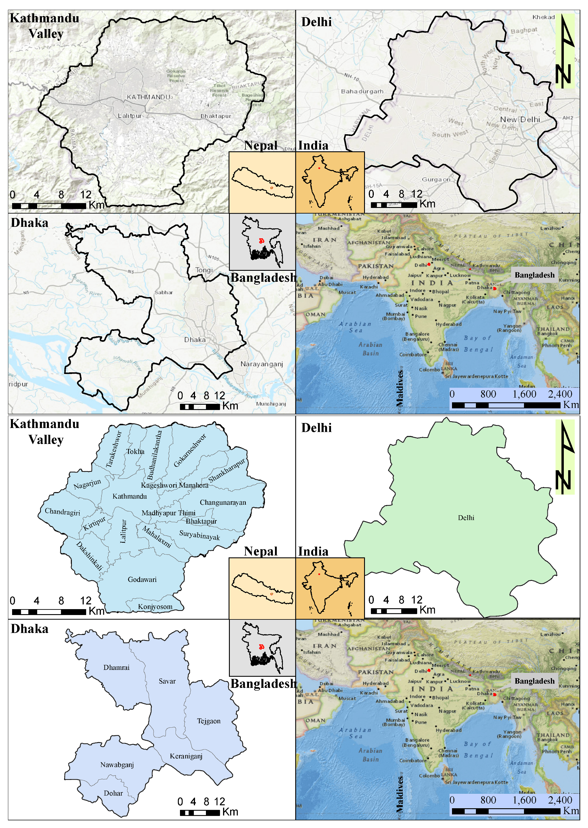
The spatial and temporal characteristics of LST, NDVI, and NDBI and their relationship has been quantified at the global and regional scale. However, these association differ between cities due to their unique geophysical, climate, and urban growth characteristics. Research has been carried out in understanding the local climate of some cities in India, however, no such study has been done for countries like Nepal. Understanding of the urban climate behavior using the satellite images in major populated and urbanized cities of South Asia is still lacking. This study aims to evaluate LST, NDVI, and NDBI and explore their associations to fill the gap and advance our understanding for the region. We have chosen three capital cities with growing populations-Kathmandu Valley (KV), Delhi, and Dhaka-to represent the region. However, such quantification of LST and SUHI (hereafter referred to as UHI) should help in planning other smart resilient cities in the region.

2. Materials and Methods

2.1. Materials

2.1.1. Landsat–8 Data

We used Landsat 8 satellite images, OLI (Operational Land Imager) and TIRS (Thermal Infrared Sensor) 15 to 30-m multispectral data from Landsat–8 C1 Level-1, downloaded from United States Geological Survey (USGS). Thermal band, Band 10, is provided as the atmospheric brightness temperature in Kelvin (K), and the multispectral-bands of Landsat–8 OLI is provided as surface reflectance. Band 10 is available at 100m horizontal resolution. Since the UHI effect is weakened by cloud cover [36], the satellite imagery with cloud coverage <10% were selected (cloud-free). Cloud cover in the entire study area is not similar. Data was selected to maintain temporal uniformity over the study period (Table 1). This data selection should not be hindered as our study focused on LST variations and UHI over modified land use rather than the absolute value of LST. A comprehensive outline of the necessary metadata is outlined in Table 1. Data required were downloaded from Earth Explorer [37] and masked to the study area. Then, the LST map for each study area was generated for different data acquisition dates as shown in Table 1. The extracted images for most of the years were obtained for summer (March-August) so that the high surface temperatures could be captured. Since we filtered the cloud cover to be less than 10%, the downloaded satellite image could not coincide for the same day in each year and most of the images were acquired for March. The scaling-factors used for determining LST and UHI were extracted from metadata (K1 = 774.4483, K2 = 1321.0789, ML = 0.0003342, AL = 0.1, please refer to Section 2.3.1 for details).

2.1.2. Population Distribution

The annual population distribution in the KV, Delhi and Dhaka is shown in Table 2 [38]. The increase in average rates of the population for KV, Delhi and Dhaka were found to be 3.97%, 3.25%, and 3.61% respectively, the highest being in KV. The rate of population change increased until 2014, then decreased until 2017, and again increased in the year 2018 for KV whilst remained constant throughout the study period for Delhi and Dhaka except in the year 2019. The rate of population change is expected to drop to 3.49% for KV, 3.03% for Delhi and 3.56% for Dhaka in the year 2020. Table 2 shows the increasing population trend for all study areas which could eventually impact the land use pattern and the surface temperature. The rapid increase in the urban population in two decades has led to the rise in the rate of urbanization too in these cities.

2.1.3. Observed Air Temperature

The average observed air temperature acquired [39] for all the study areas is shown in Table 3. The observed temperature for the missing satellite data acquisition months in 2015 and 2018 for Delhi were obtained on 28 July 2015 and 20 June 2018 respectively. Likewise, the observed air temperature for Dhaka in 2013 was obtained on the day of 20 March 2013. Meanwhile, the missing temperature data on the satellite data acquisition day were obtained by averaging the temperature from the previous day and the following day of the missing date.

2.2. Study Area

South Asian (SA) nations, namely: Afghanistan, Pakistan, India, Nepal, Maldives, Bhutan, Sri Lanka and Bangladesh combined have more than 18 billion population [40] where 31% resides in the urban area [41]. The capitals of SA nations are economically rich, urbanized, and highly populated. Delhi (30.2 million) and Dhaka (21.0 million) are the top 10 most populated capital cities in SA, while KV is the most populated and emerging urbanized city in Nepal. The rising population has induced urbanization in all these capitals. The rate of urbanization is increasing rapidly with the increase in population to 130 million in just a span of 10 years (2001 to 2011) and is expected to reach 250 million by 2025 [42] in SA. A brief description of each study area is discussed below under each sub-sections. The section deals with the physiography and climate of each study area.

2.2.1. Kathmandu Valley

KV is one of the biggest cities, in terms of population and economic development, in Nepal comprising an area of approximately 664 km2 (Figure 1). The bowl-shaped valley is located at 85 11 E 27 32 N inscribing the major cities Kathmandu, Lalitpur and Bhaktapur [43,44]. KV lies in the warm temperate zone [45] with a fair climate varying from 2.4 C to 37 C in the period of 1981–2010 [46]. Geographically, the central lower part of the valley is situated at an elevation of 1425 m above mean sea level MSL and is surrounded by four mountain ranges namely Shivapuri, Phulchowki, Nagarjun, and Chandragiri Hills. KV is the most developed city in Nepal with a greater portion occupied by the built-up area. On the contrary, KV has some open spaces namely Tundikhel, Tribhuvan park, Sankha park, etc., which are expected to serve as green space thereby reducing the rising daytime temperature.

2.2.2. Delhi

Delhi located in Northern India, at 77 14 E 28 36 N is bordered by Uttar Pradesh in the East and by the states of Haryana on the West, North and South (Figure 1). It covers an area of 1484 km2, of which 783 km2 is designated as rural, and 700 km2 as urban therefore making it the largest city in terms of area in India. It has a length of 51.9 km and a width of 48.48 km. Delhi has a dry subtropical and semi-arid type of climate [47]. The annual average temperature is 25 C with monthly means varying from 13 C to 32 C. The warm season begins in early April and peaks in late May or early June with an average temperature of about 38 C but occasional heat waves may result in high temperatures of over 45 C on some days. Per capita availability of green space in Delhi is about 20 m2 whereas that of open space is 30 m2 [48].

2.2.3. Dhaka

Dhaka is located in central Bangladesh at 90 22 E 23 42 N (Figure 1) along the eastern banks of the Buriganga River. The city lies on the lower reaches of the Ganges Delta and covers a total area of 306.38 km2. Dhaka has a tropical savanna climate. The city has a distinct monsoonal season, with an annual average temperature of 26 C and monthly means varying between 19 C in January and 29 C in May [49]. There are many parks within Dhaka city, including Ramna Park, Suhrawardy Udyan, Shishu Park, National Botanical Garden, Baldha Garden, Chandrima Uddan, Gulshan Park, and Dhaka Zoo. There are lakes within the city, such as Crescent lake, Dhanmondi lake, Baridhara-Gulshan lake, Banani lake, Uttara lake, and Hatirjheel-Begunbari lake. These parks and lakes act as green space and help in minimizing the rising surface temperature.

2.3. Methodology

Figure 2 shows the flowchart of methodologies adopted in this study. A step-wise description is discussed below:

2.3.1. Step-Wise Methodologies to Estimate UHI

Conversion of Spectral Radiance to Top of Atmospheric Brightness Temperature

Landsat 8 satellite imagery obtained was processed using 32-bit floating-point calculations. These values were then converted to 16-bit integer values in the finished level 1 product. Conversion to spectral radiance was done using the radiance scaling factors provided in the metadata file [37] using Equation (1).
L λ = M L Q c a l + A L
The calculated spectral radiance was then converted to brightness temperature which was often determined as the effective temperature under unit emissivity. Top of Atmosphere (TOA) Brightness Temperature was obtained from spectral radiance in degree Celsius using Equation (2).
T B = K 2 L n K 2 L λ + 1 273.15
where,
  • L λ = TOA spectral reflectance (watts/(m2 * sr * μ m)),
  • ML = Band specific multiplicative rescaling factor,
  • Qcal = Quantized and calibrated standard product pixel values (DN),
  • AL = Band specific additive rescaling factor,
  • TB = Effective temperature in C

Landsat Surface Temperature Generation

OLI and TIRS band data were converted to radiance using the radiance scaling factors provided in the metadata file using Equation (1) and then to TOA brightness temperature using Equation (2). After acquiring brightness temperature, L S T for Landsat–8 was estimated using Equations (3)–(7). Parameters such as N D V I , proportion of vegetation (Pv), and ground emissivity (e) were required to estimate the L S T . Each parameters N D V I , Pv and e were calculated using Equations (4), (6), and (7) respectively. N D V I was calculated using Near InfraRed Band (B5) and Red Band (B4) of Landsat imagery. Normalized Difference Built-up Index ( N D B I ) was calculated using 6th (Middle InfraRed) and 5th (Near InfraRed) of Landsat 8 bands using Equation (5).
L S T = T B 1 + ( λ T B C 2 ) L n ( e )
N D V I = B 5 B 4 B 5 + B 4
N D B I = B 6 B 5 B 6 + B 5
P v = N D V I N D V I min N D V I max N D V I min 2
e = 0.004 P v + 0.986
where,
  • L S T = Land Surface Temperature ( C),
  • TB = Effective temperature ( C),
  • N D V I = Normalized Difference Vegetation Index calculated using Equation (4),
  • N D B I = Normalized Difference Built-up Index calculated using Equation (5),
  • Pv = Proportion of vegetation calculated using Equation (6),
  • e = Ground Emissivity calculated from Equation (7),
  • λ and C2 are constants having values of 10.8 and 14,388 respectively.

Urban Heat Island

After obtaining LST, Equations (8) and (9) were used for determining UHI used by Kaplan et al. [34]. Here, μ is the mean LST value for the study area, and σ is the standard deviation of the LST.
U H I = L S T > μ + 0.5 σ
U H I = 0 < L S T μ + 0.5 σ

3. Results

3.1. LST, NDVI, and NDBI for Each Study Area

3.1.1. Kathmandu Valley

The estimated spatial distribution of LST for KV is shown in Figure 3 and Figure 4 for the dates reported in Table 1. We observed an increase in surface temperature up to more than 30 C for 2015 and 2018. In the year 2015, LST was estimated for June so most of the region in KV had higher temperature compared to other years. Kathmandu and Lalitpur Metropolitan City (referred to as Kathmandu and Lalitpur) showed higher surface temperature compared to other nearby municipalities (Madhyapur Thimi, Kirtipur etc.) and rural municipalities (Konjyosom) (refer Figure 1 for the locations of administrative units). It may be noted that in June 2015, Konjyosom rural municipality exhibited higher temperature than in other years.
The peri-urban municipalities like Nagarjun, and the higher region of Budhanilkantha, and Godawari had the temperatures ranging from 15 C to 25 C most of the years. These regions also had surface temperature higher than 27 C during 1 June 2015, 22 April 2018, and 8 May 2018. This might be due to the rise in air temperature as a result of reflectance in the urban and barren land. Kathmandu and Lalitpur experienced higher temperature most of the summer time. However, the boundaries of KV such as Chandragiri, Dakshinkali, Nagarjun, Gokarneshwor, Budhanilkantha, and Konjyosom experienced temperatures less than 10 C.
The second and third columns of Figure 3 and Figure 4 show the temporal and spatial distribution of NDVI and NDBI for KV. The figures depicted that vegetative area (NDVI > 0) was higher in the peri-urban area compared to central KV which had NDVI < 0, negative NDVI for March 2013 and 2014. NDVI values for central KV were negative which support the presence of non-vegetative areas usually barren land or built-up area. It was observed, as expected, that the built-up area increased with the increase in population.
Further, the result of NDBI confirmed that the built-up area (NDBI < 0) was concentrated in the central KV, mainly in Kathmandu, compared to peri-urban areas of KV such as Godawari and Nagarjun municipalities. Central KV, including Kathmandu and Lalitpur, had lower values of NDVI and higher values of NDBI which states that it KV was less vegetative compared to other regions. NDVI ranged from −0.1 (March 2016) to +0.6 (June 2015) during the study period in KV. Most of the peri-urban regions within KV had higher values of NDVI during 2015 while central KV showed a lower value of NDVI. Similarly, NDBI in KV ranged from −0.2 to +0.4. Most of the built-up areas were concentrated in central KV while the peri-urban areas had lesser built-up areas as shown in the third column of Figure 3 and Figure 4. Expansion of NDBI further demonstrates that the built-up areas in the eastern KV were increasing. Change in the land cover pattern such as the increase in impervious areas (attributed by increase in NDBI values) has limited the recharge capacity of the groundwater in central KV [50,51] which eventually reduces the soil moisture.
The estimated average surface temperature ranged from 20 C in 2016 to 32 C in 2015 (Table 4). The higher discrepancy in observed and estimated temperature occurred in the year 2017 and 2019 resulting in higher differences of 5.04 and 5.3 C, respectively. While the discrepancies in other years were found to be comparatively less as shown in Table 4.

3.1.2. Delhi

Spatial and temporal distribution of LST, NDVI, and NDBI for Delhi is shown in Figure 5 and Figure 6. In the eastern end of Delhi two areas were not well characterized by the satellite imagery, dark blue color on the right side for the year 2013–2016 and lower left for the years 2017 and 2019. We did not consider and these two areas for the analysis. LST for Delhi ranged from 15 to 30 C in most of the regions during 2013–2017 while very few areas experienced LST > 35 C. However, the reverse was the case for the year 2019 where most of Delhi received surface temperature > 35 C, except for the Yamuna river ranging from 25 to 30 C. The comparison of observed and estimated LST Table 5 showed that the maximum difference in the temperature was 9.3 C in the year 2017, whereas the least bias of 2.3 C found in the year 2019.
LST in Delhi was found to be inconsistent intra-annually. During the year 2013, June was considered for the evaluation purpose and the mean surface temperature was found to be 32.8 C with minimum and maximum LST being 14.7 C and 42.9 C, respectively. Areas in the north of Delhi experienced the minimum temperature while the south-west region exhibited the maximum temperature. Most of the regions in Delhi had LST ranging from 30 to 35 C as shown in the upper panel under the LST column in Figure 5. However, in 2019, mean LST was estimated to be 40.2 C with minimum and maximum LST to be 29.8 and 47.7 C respectively. The higher LST may be attributed to the increase in the built-up area, also demonstrated by the NDBI. In contrast, the south-east part of Delhi shows reduction in the LST values which may be an artifact of data processing. The maximum value of NDBI in 2019 was found to be 0.51 which increased from 0.29 in 2013. Similarly, the result of NDVI showed a decrease in the maximum vegetative index from 0.47 in 2013 to 0.44 in 2019.
The result of NDVI portrayed that vegetative area was less compared to non-vegetative areas. The non-vegetative area increased with the increase in LST. The vegetative area was more in south Delhi compared to north Delhi which holds more built-up towns and industrial areas. However, in, 2016, NDVI map showed that Delhi has a more vegetative area compared to non-vegetative which might be the result of lesser air temperature (observed 33.5 C) and higher relative humidity (RH) compared to 2015 and 2017 for the same month. RH was found to be 21% in the data acquisition day in 2019.
Similarly, 40 C observed temperature and 30% RH, was observed in 2013. NDVI values ranged from −0.09 in 2013 to 0.52 in 2016 (August). This suggested that Delhi has a lesser vegetative area compared to the non-vegetative area. A similar pattern was observed from NDBI. Most regions in Delhi have NDBI value ranging from −0.3 to 0.51, the distribution shows higher percentage of the built-up area than the non-built-up area. The NDBI values suggest that more areas in Delhi radiate the incoming sunlight thereby increasing the temperature of the study area.

3.1.3. Dhaka

The spatial and temporal distribution of LST, NDVI, and NDBI were plotted for Dhaka district as shown in Figure 7 and Figure 8. The spatial distribution of LST over Dhaka showed the temperature distribution in March 2014 was higher than 35 C, a few areas have a temperature less than 35 C. This was validated by the observed temperature as shown in Table 6. The bias in observed air temperature and estimated surface temperature was found to be −1.23 C in the year 2014. The maximum bias of +5.5 C was found in 2018.
The spatial distribution of NDVI showed that most of the western districts in Dhaka such as Dhamari, Savar, Nawabgang and Dohar are vegetative compared to eastern districts such as Tejgaon and Keraniganj. It further showed that during the years 2016 and 2017, the non-vegetative area has increased in the eastern districts. The similar pattern was observed from the NDBI too. The eastern districts are highly built-up in comparison with the western. The NDBI values ranged from −0.10 in the year 2019 to +0.55 in the year 2018. Negative values of NDBI showed a non-built-up region while the positive value reflected the built-up area of the study area.

3.2. Relationship between LST, NDVI and NDBI

The relationship between LST, NDVI and NDBI is necessary to understand the UHI phenomenon in urban cities. Increase in the LST values is governed by the climatic (rainfall, air temperature, humidity) and non-climatic (land use and land cover, aerosols, air particles in the atmosphere, built-up area) variables. Spatial average values of LST, NDVI, and NDBI were used to understand the relationship between them.

3.2.1. Kathmandu Valley

The relationship between LST and NDVI showed a mixed relation trend for KV. The negative linear trend exists for temperature less than 25 C and the parabolic relationship for higher values with p-value = 0.08 (p-value > 0.05) and R2 = 0.05. The statistical performance of p-value shows that there is no statistically significant relation between mean LST and mean NDVI. The non-vegetative area increased with increment in the surface temperature (Figure 9). This implies that likely the increase in non-vegetative areas is directly associated with the change in surface temperature and built-up area [26]. For the surface temperature ranging from 22.5 C to 30.0 C, the NDVI increased. This indicates an increase in greenness together with an increase in surface temperature. This variation might be attributed to rainfall days before the measurement was taken.

3.2.2. Delhi

The relationship between mean LST and mean NDVI was established for the study period 2013–2019 as shown in Figure 10. The statistical performance of the relationship among mean LST and mean NDVI shows a negative linear trend with R2 value of 0.79 and p-value = 0.043 (p-value < 0.05). This shows a statistically significant relationship between mean LST and mean NDVI. Since Delhi is often viewed as a single administrative unit, we have used only 5 temporal data points to develop the relationship. The Figure 10 shows the well-distributed relationship between mean LST and NDVI (R2 = 0.79). The increase in mean LST was concomitant in the decrease in vegetative area for Delhi. Thus with the increase in the surface temperature, the number of UHI regions are likely to increase. This situation might exacerbate the risk of heat-stroke in Delhi.

3.2.3. Dhaka

Relationships between mean LST and mean NDVI were studied for Dhaka district and found that NDVI value increased slightly with the increase in LST. The statistical result shows very low correlation exists between mean LST and mean NDVI (R2 ∼ 0). The p-value is equal to 0.75 (p > 0.05) is not statistically significant and cannot provide enough evidence for rejecting the null hypothesis of similarity. During data acquisition day in 2014–2019, most of the administrative units had mean LST ranging from 24.0 C to 28.0 C with the variation of NDVI ranging from 0.0 to 0.35 (Figure 11).

3.3. UHI for the Study Area

UHI was calculated based on mean and standard deviation (SD) of LST. Green color shows the non-UHIs while red color shows the UHI regions for each of the study areas. The threshold value of UHI ranged from 21.6 C to 24.2 C for KV, from 26.2 C to 41.3 C for Delhi and from 24.6 C to 34.9 C for Dhaka (Figure 12, Figure 13 and Figure 14 respectively). The variation in the UHIs was governed by the LST each land cover type had in the study area. Further, the availability of green space (as seen from NDVI) and clustering of the built-up area (as seen from NDBI) have a significant impact on the UHI for each study area.

3.3.1. Kathmandu Valley

The spatial and temporal distribution of UHI for the KV was developed for each year using the surface temperature for the same month (Figure 12). Distribution of UHI showed that for all the years, central KV experienced higher temperature and thus may be considered as heat islands which were further supported by LST, NDVI and NDBI in earlier sections. Compared to southern regions, the Northern region is highly populated (as can be seen from NDBI maps) and thus these regions experienced higher temperatures. On 26 March 2013, the central and Northern region experienced temperatures higher than 28.3 C. The boundary administrative such as Budhanilkantha, Gorkarneshwor, Changunarayan, Godavari, Chandragiri, etc. had comparatively lesser UHI effects throughout the study period. The result of UHI analysis also show an increasing trend in UHI especially in the peri-urban areas. Spatial analysis revealed that the UHI zones were more concentrated in the central and northern regions of the KV. UHI at the different administrative units of KV reflected the increasing trend of UHI zones which might be the impact of increasing population and intensified urbanization. Developing the new greener space might help in reducing the impact of increasing UHI in the densely populated urban cities like KV [52].

3.3.2. Delhi

Figure 13 showed the spatio-temporal distribution of UHI for Delhi. The minimum threshold of UHI for Delhi was found to be 26.2 C in the year 2016 on the data acquisition date. The maximum threshold of UHI was estimated to be 41.3 C for the year 2019. With the higher values of mean LST and the least value of SD, most of the areas in Delhi are estimated to behave non-UHI. Since the UHI threshold is less and the temperature range is small, more UHI areas were observed in Delhi in 2016 compared to other high UHI threshold years. This point to a limitation of UHI threshold for cities like Delhi. Residential or mixed regions have a higher potential risk of UHI in Delhi as portrayed by Mohan et al. [53]. Researchers [53] further stressed that UHI in summer is expected to increase and become more dominant in the densely urbanized built-up areas.

3.3.3. Dhaka

The minimum and maximum threshold of UHI for Dhaka were found to be 24.6 C and 34.9 C respectively (Figure 14). The result showed that western districts such as Dohar, Nawabganj, Dhamrai behave as non-UHI while the eastern districts such as Tejgaon, Savar, and Kernaiganj behave as UHI zones. The North-West region of Dhaka was less impacted by the rising surface temperature and is thus identified as non-UHI regions throughout the temporal study period. Eastern parts of Tejgaon and Keraniganj were identified as UHI regions for each year is associated with a higher density of impervious structures such as concrete buildings and paved roads in the region. The potential impact of UHI is increased by the rising surface temperature in the Dhaka city from 28.5 C in 2002 to 40.1 C in 2014 [54].

4. Discussions

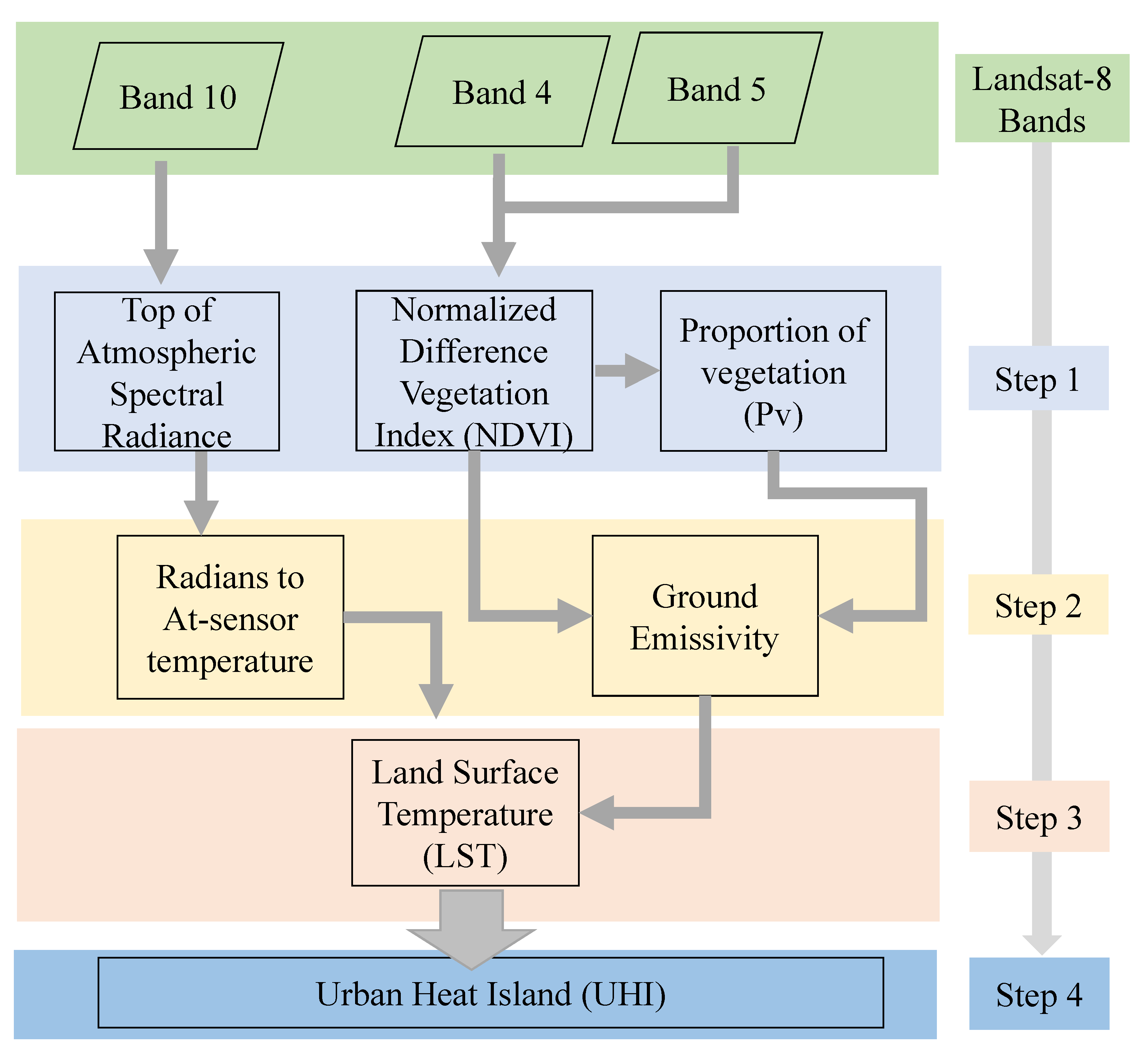
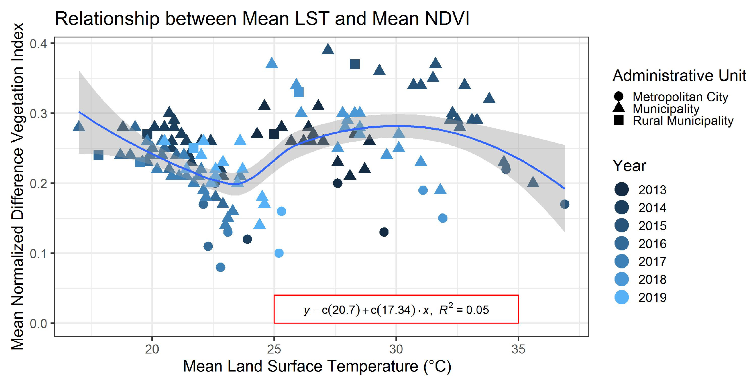
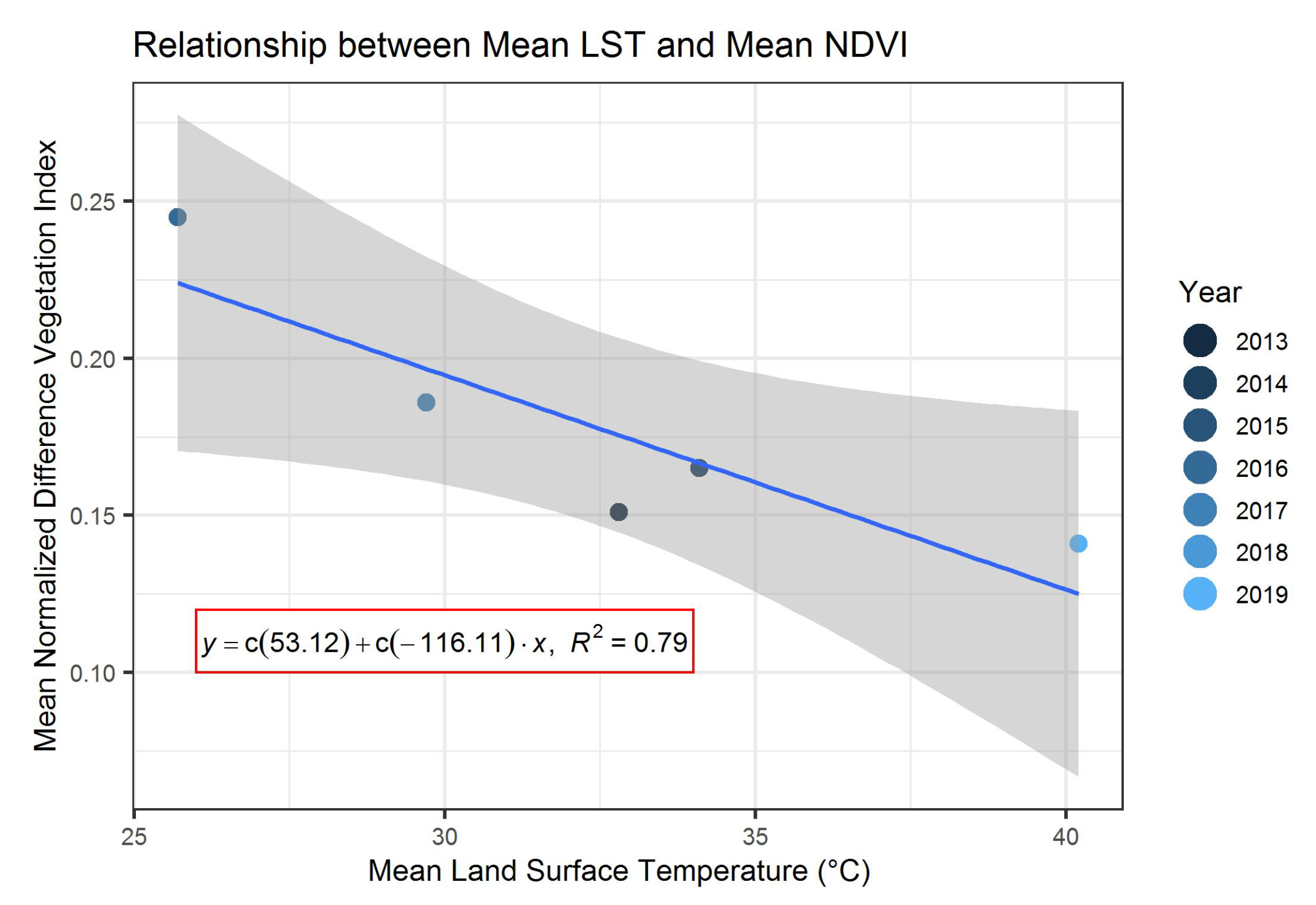
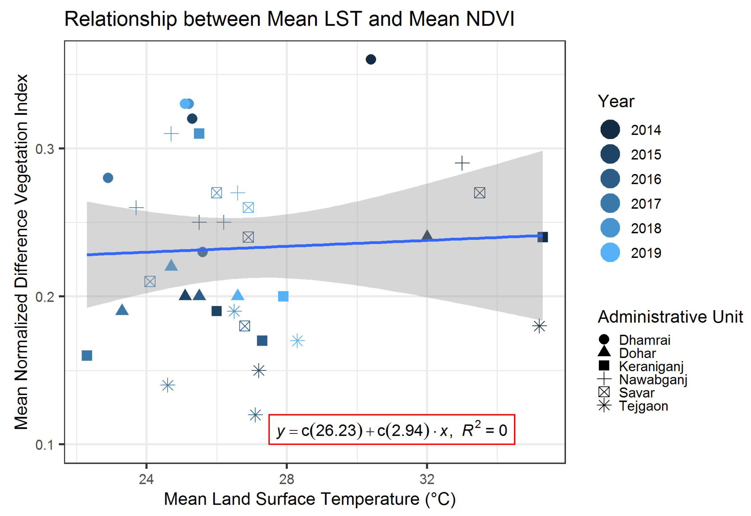
Satellite imageries provide an appropriate platform to evaluate LST and UHI at any spatial and temporal scale. The primary objective of the study is to evaluate the UHIs in densely populated cities of South Asia namely, Kathmandu, Delhi, and Dhaka using satellite imageries. Also, we examined the LST, NDVI, and NDBI for the same to observe the state of surface temperature, wetness, and dryness of the land and Built-up intensity for the temporal period of 2013–2019.

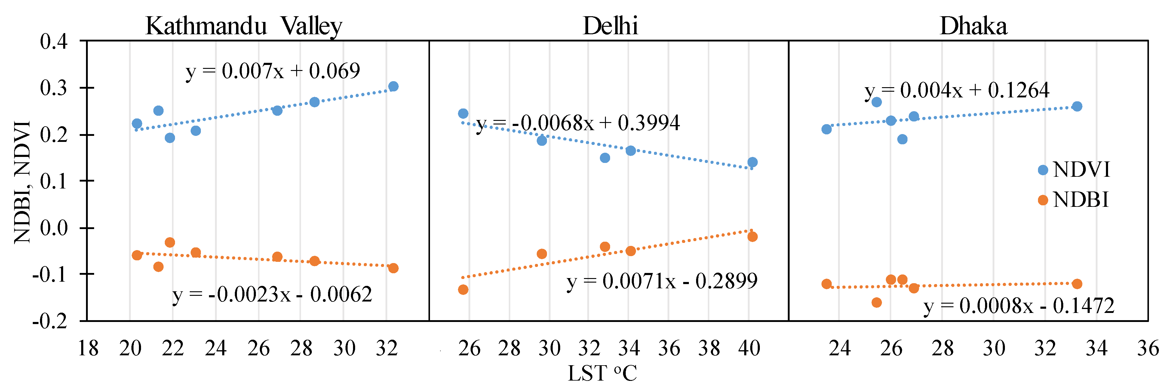
4.1. Relationship between LST, NDVI and NDBI

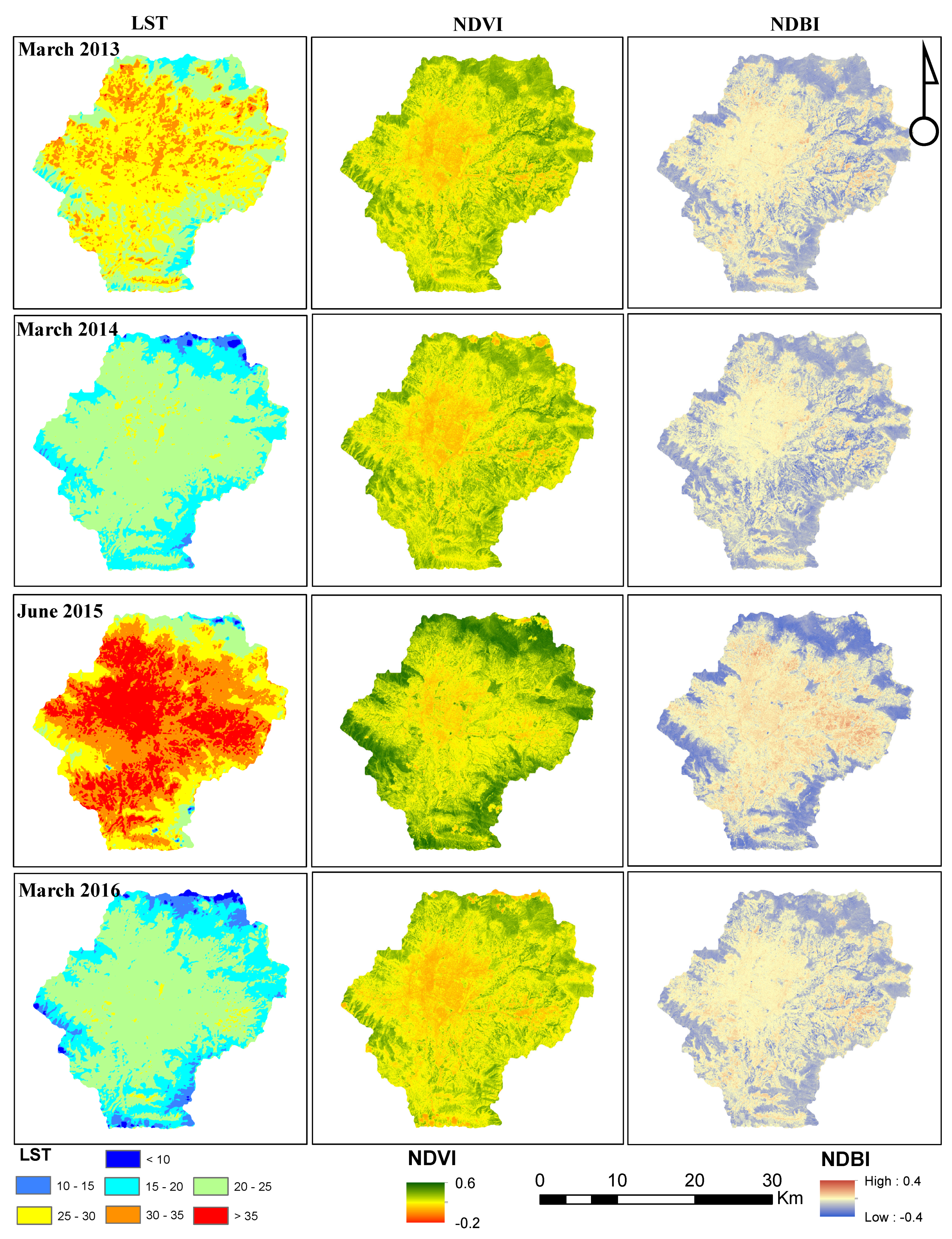
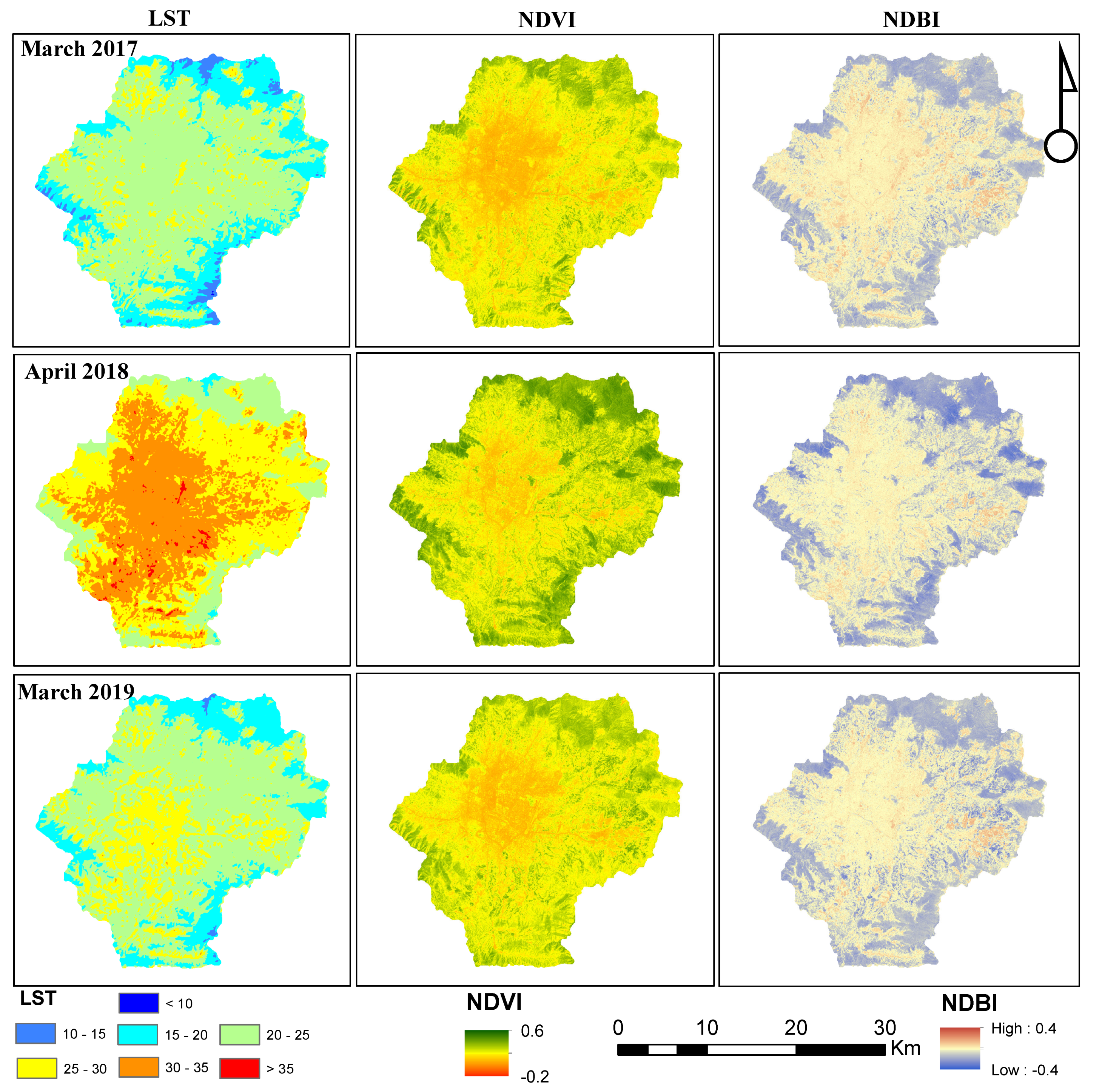
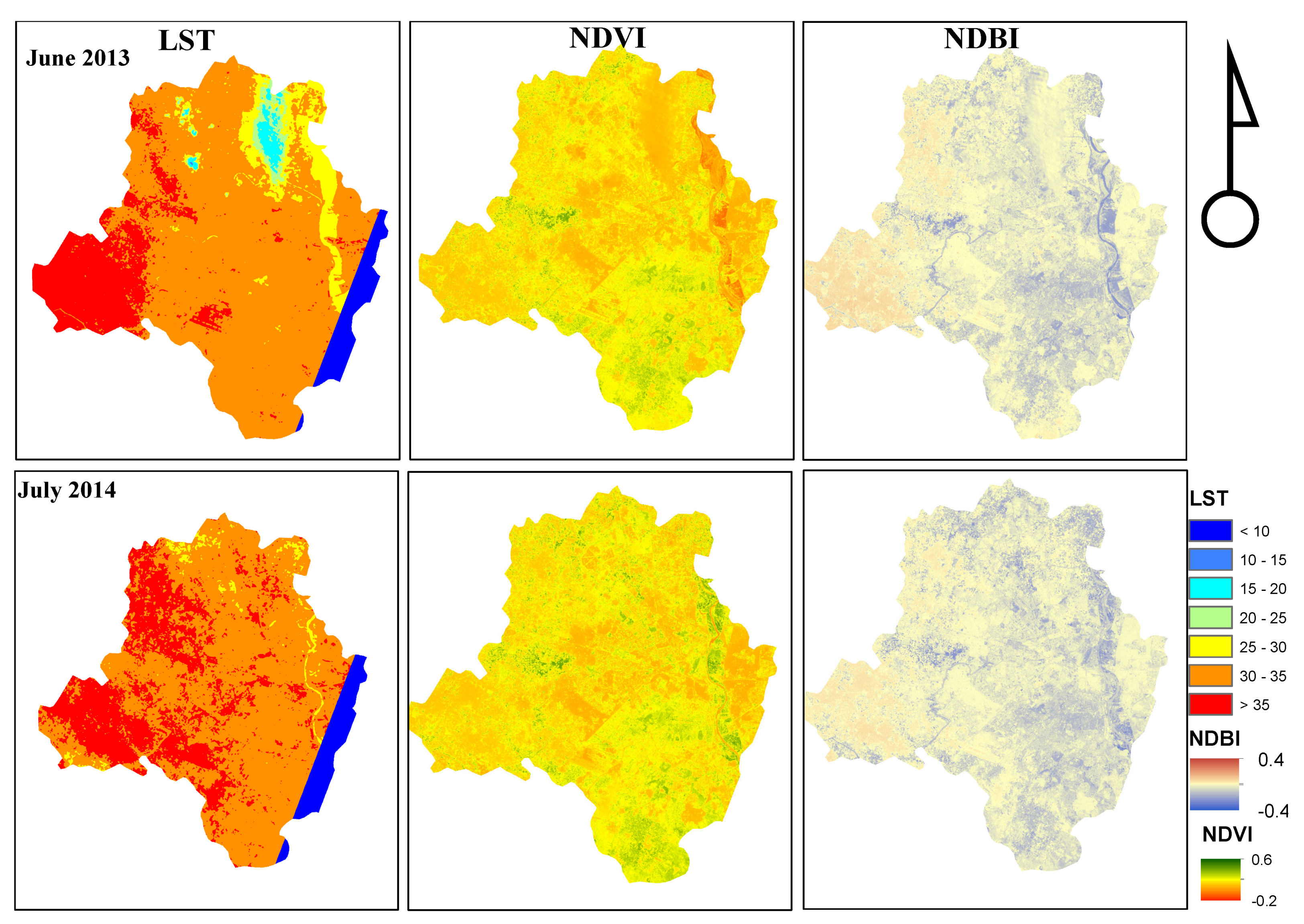
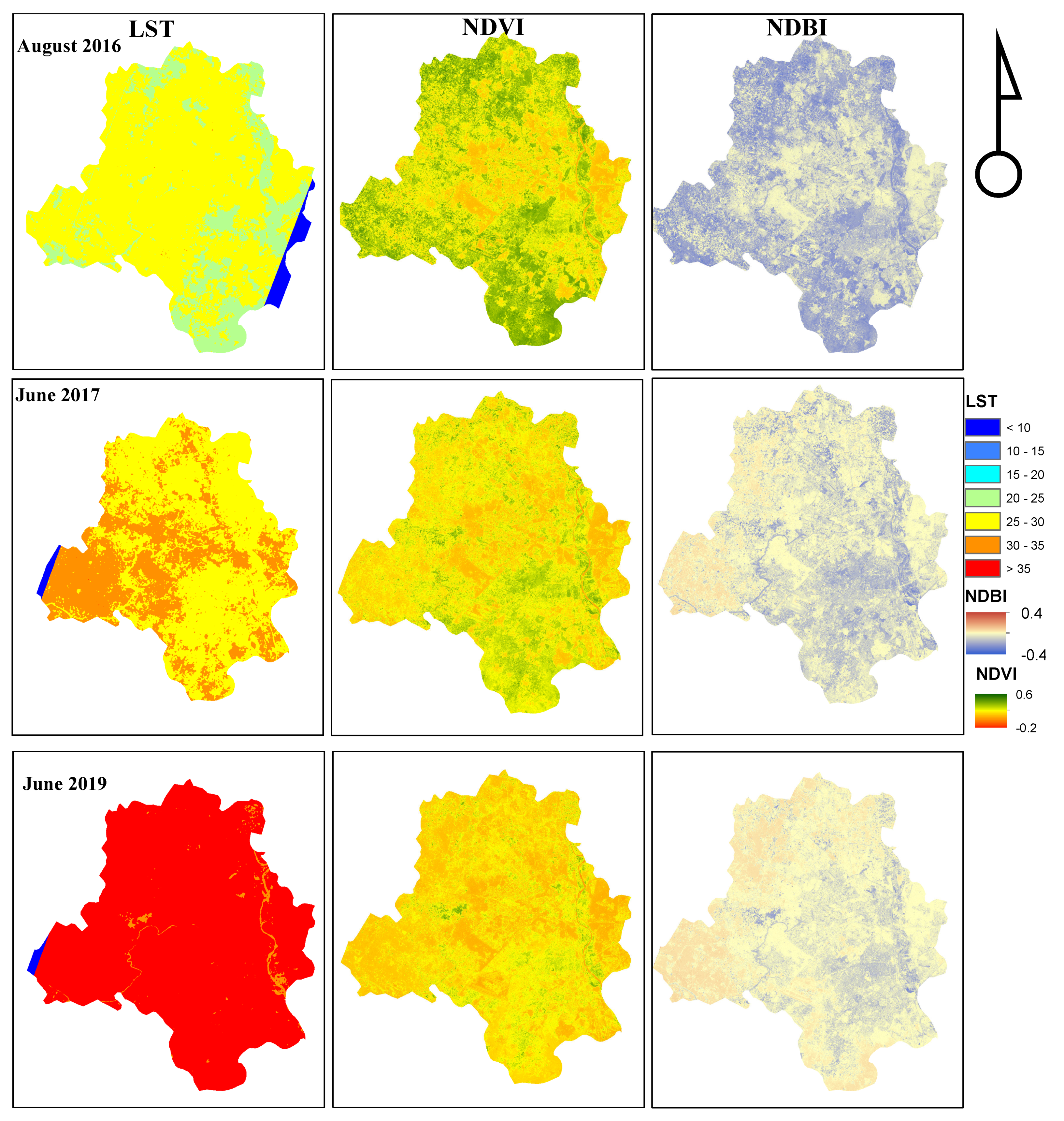
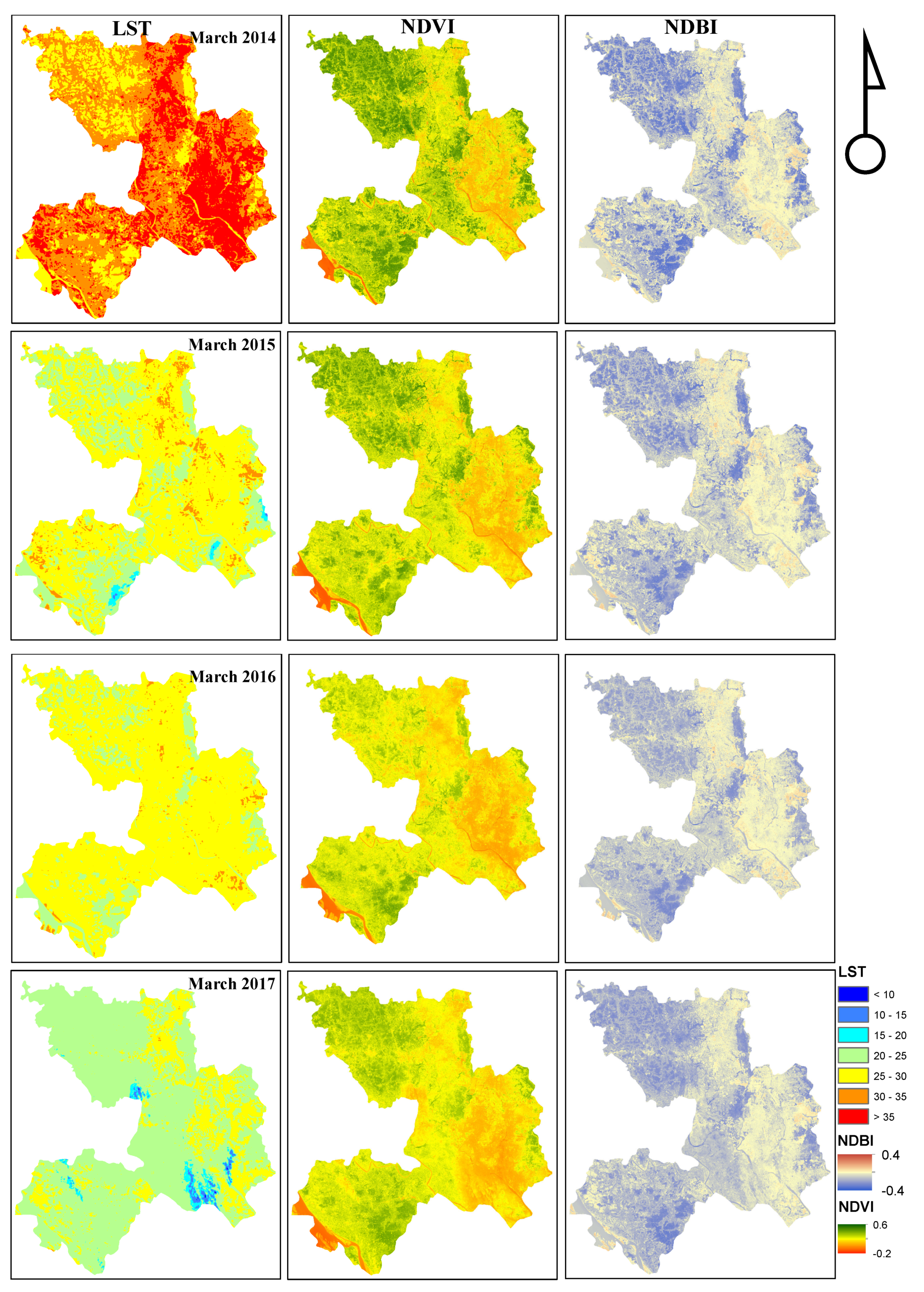
Visual analysis of the LST showed that June 2015 was the most hottest month during the temporal study period in KV. In 2014 and 2016, the month of March was found to have less warm days in the high elevated regions where the LST is <10 C (Figure 3 and Figure 4). In the case of Delhi, high LST was observed in 2019 followed by 2013 and 2014. Similar trends of the LST variation were observed in Dhaka. NDVI values for KV and Dhaka were found to increase at the rate of 0.007 and 0.004 respectively while a negative trend was observed in Delhi (Figure 15). The negative trend in Delhi might be the result of the presence of a relatively higher amount of the open spaces as compared to KV and Dhaka. The results depict an increasing trend of NDBI values for Delhi; almost no trend for Dhaka and decreasing trend for KV (Figure 15). The spatio-temporal variation in the NDVI and NDBI values might be the consequences of the local climatic conditions [55] of the study area. The spatio-temporal variation over the different topographical regions has been well established in the study domains. Climates of the study area have an important role in governing LST, NDVI, NDBI, and UHI as computed in this study. The large orographic differences over a short latitude change could be responsible for lesser LST and higher NDVI values in the KV [45,56,57]. The differences in spatio-temporal LST retrieval in the study domain might have been affected by the biophysical effects, evapotranspiration, and albedo that are eventually influenced by precipitation and local climate [58]. Densely populated zones in the study areas are found to have higher LST values compared to surrounding areas. The higher values of LST in the central zone of the study area is likely due to the densely built-up area and paved roads [26,59]. Pan et al. [60] found that the LST values at built-up areas are higher than 40 C in the humid subtropical climate. The variation in LST was also attenuated by the change in elevation. Increase in the LST values was also concomitant with increased population in all the cities of South Asia [61].

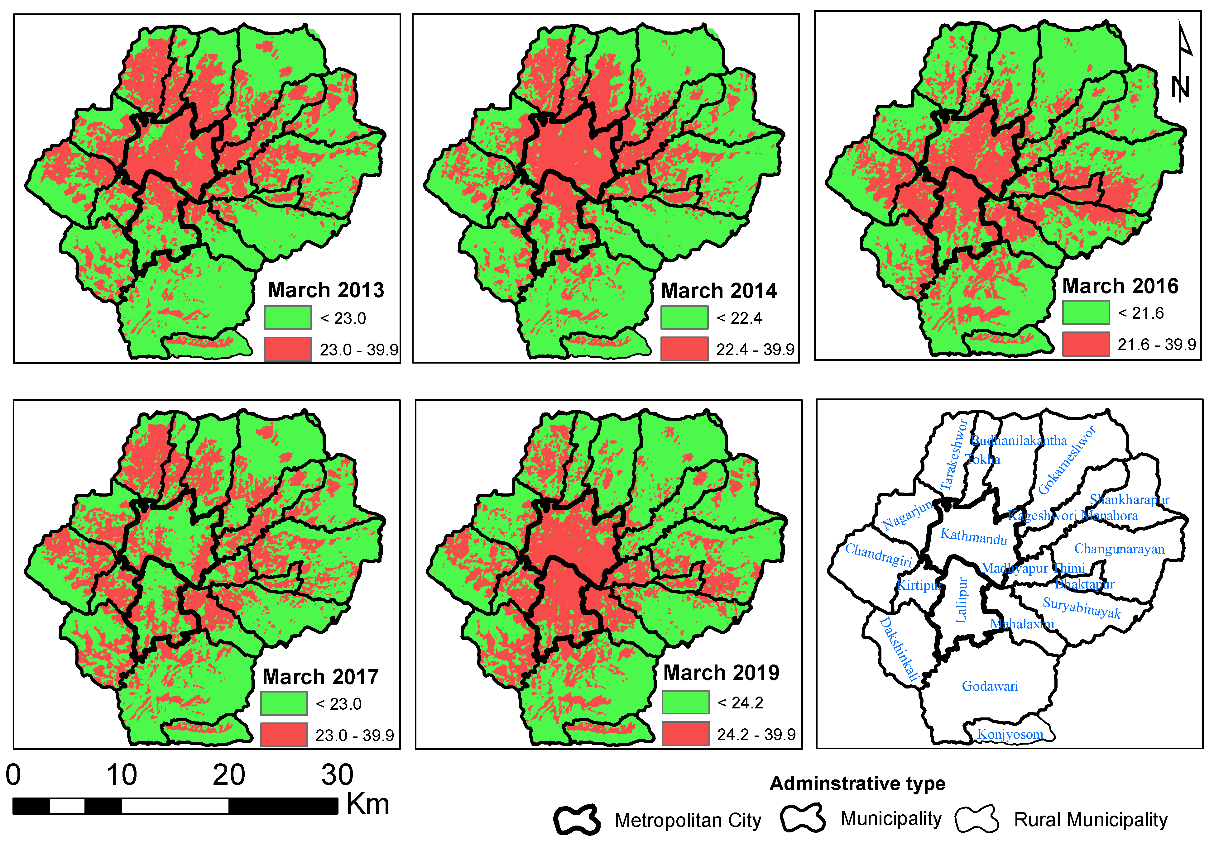
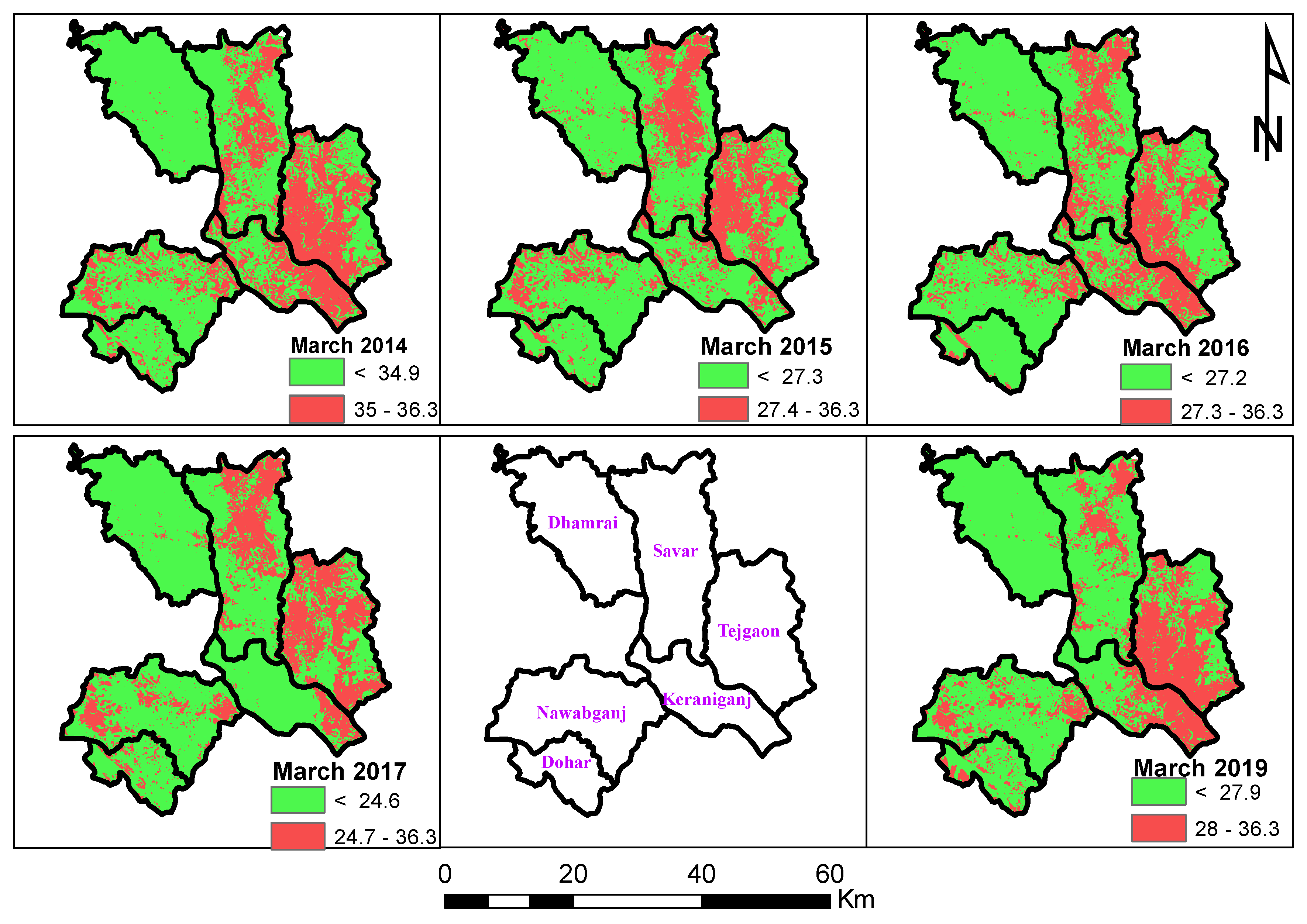
4.2. Quantification of UHI from Retrieved LST

UHI values retrieved for the study areas showed the increment in UHI zones with the passage of time. In KV, the lower UHI values ranged from 21.6 C in 2016 to 24.2 C in 2019 while the maximum reached 40 C. The lower UHI values for Delhi varied from 26.2 C in 2016 to 41.3 C in 2019. Similarly, the lower UHI values for Dhaka varied from 24.6 C in 2017 to 34.9 C in 2014. The business centers attributed by economic conditions [62] and increased population [63] in each study area were found to have higher UHI values compared to surrounding areas. The increased built-up areas and the paved roads might be the driving factors that alter the spatio-temporal alteration of UHI zones. Further, the reduced open spaces (green areas) and current development works such as the construction of roads, buildings might have aggravated the increase in the UHI zones. Growth and development activities increases the impervious surfaces, resulting in reduced evapotranspiration and lesser soil moisture [64], which ultimately have a direct impact on the LST of the urban areas. The spatio-temporal variation in UHI values across the study area has been impacted by increased NDBI index [34]. UHI magnitudes increased across the regions with increased NDBI and decreased NDVI. El Niño might also have contributed to the wider variability of UHI effects in the study regions [65].

4.3. Impact of UHIs and Mitigation Strategies to Minimize Rising Surface Temperature

The UHIs has diverse impacts on different elements of the society such as energy consumption, human health, biodiversity, agriculture, water availability and others [66]. With the increase in the urban population (Table 2) and urbanization, the intensity and frequency of the heatwaves have increased. Further, an increase in the frequency and magnitude of hotter days attributed by the rise in LST and UHI zones have a direct impact on the energy consumption. The urban population tends to consume more electricity to make themselves more comfortable against the increasing heat. In recent years, the trend of electricity consumption in SA region is increasing [67,68]. The increase in electricity consumption might be the cumulative impact of the increasing population, rising urbanization, growing wealth, and climate extremities. Further, the increased climate extremes (such as heat strokes, UHI, increased LST) has also impacted the health of the people in SA. The comfort level induced by the climatic extremes in the health of the residents of any city is measured in terms of discomfort index (DI) and physiological equivalent temperature (PET) index. The previous research in SA and West Bengal (India) showed that the area with shades due to high rise buildings and trees have comfortable conditions compared to the one with no shades [66,69]. The increase in surface temperature has increased the number of heat strokes in urban cities of SA [70]. The number of patients suffering from heat stroke was found to be comparatively higher in the urban centers than in the peri-urban areas of SA. This supports the idea that increasing UHI and LST has increased the risk of heatwave globally and regionally [71,72]. The increased surface temperature has a significant impact on diarrheal disease and heat stress in Bangladesh [73]. The policy makers and planners of each study region now need to focus on the proper mitigation and adaptation strategies to cope against the rising LST and increasing UHIs. This study shows that more planning and perhaps enforcement are required to reduce the impact of the rising surface temperature. Increase in the green land area and afforestation activities can reduce the impact of excess heating from the solar radiation. This also enhances the asthetics of the city. Few mitigation strategies have been considered by the local government in Kathmandu valley such as cleaning of the Bagmati river corridor and increasing the number of new recreational parks. In India, Niti Aayog has proposed to ban the diesel vehicle and sell the electric vehicle by 2030 to reduce the air pollution. Such major mitigation measures are necessary for reduction of UHI too for the region to be better prepared for climate extremities.

4.4. Limitations of the Research

The current study has limitations in the spatial and temporal domains. Temporally, we only focused on the summer days to assess the summer surface temperature and subsequent heat island. Spatially we focused on the highly urbanized and rapidly rising cities at SA. The study focused on three major cities, however several smaller cities in SA may face similar problems. A coordinated effort is needed to understand the regional LST and UHI in detail. Also, understanding of antecedent conditions coupled with on ground sensing may be beneficial for future work.

5. Conclusions

This study evaluated the UHI using the Landsat-8 satellite images in three densely populated cities of South Asia namely, Kathmandu Valley, Delhi, and Dhaka. These are the growing cities in terms of economic development, urbanization and population rise. The spatial and temporal variations of LST, NDVI, NDBI, and UHI were analyzed in these three cities to assess the impact of urbanization on the surface temperatures. An increase in the impervious areas, such as concrete buildings and paved roads reduces the recharge capacity of the soils thereby reducing the soil moisture. This leads to an increase in barren and non-vegetative lands in these urban cities. The analysis of LST and UHI in these urban cities demonstrate the importance of urban planning to mitigate the effects of future climate. The analysis was focused from 2013–2019 when the cloud cover is less than 10%. The following conclusions are drawn from the research:
  • Results of LST showed the surface temperature is more in the Kathmandu and Lalitpur Metropolitan City while the regions that are situated at the boundaries of KV experienced LST less than 10 C, below that of KV. Similarly, for Delhi higher LST is observed in the western region of Delhi and the eastern region of Dhaka. It can be inferred that the zones which are densely populated experience higher LST.
  • Like LST, NDVI of the study area shows more vegetative regions in peri-urban areas and less in the central KV. NDVI result of Delhi shows a lesser vegetative area than the non-vegetative area. In the case of Dhaka, the eastern district (Tejgaon) has less vegetative area compared to the western region.
  • NDBI shows the concentration of built-up areas in most regions of the KV (NDBI > 0). Regions with NDBI < 0 are concentrated in the peripheries of KV. Similarly, NDBI result exhibits that the built-up area is concentrated in the western region for Delhi and the eastern region for Dhaka.
  • The results of this study imply that the spatial distribution of LST magnitude and UHI zones are greater in Delhi and Dhaka compared to KV. However, the core center of the KV has a higher rate of LST magnitude and UHI effects are increasing faster annually.
  • The results of the research provide insights into urban microclimates and changes in the environment that may be used for drafting the city planning legislation to mitigate the rising LST.

Author Contributions

Conceptualization, M.M., A.A. and B.M.S.; methodology, M.M., A.A. and B.M.S.; software, M.M., A.A. and B.M.S.; validation, M.M., A.A. and B.M.S.; formal analysis, M.M., A.A. and B.M.S.; investigation, M.M., A.A., B.M.S., R.T., B.R.T., S.K.; resources, M.M.; data curation, M.M.; A.A. and B.M.S.; writing–original draft preparation, M.M.; writing—review and editing, M.M., A.A., B.M.S., R.T., B.R.T., S.K.; visualization, M.M., A.A., B.M.S., R.T., B.R.T., S.K.; supervision, R.T., B.R.T., S.K.; All authors have read and agreed to the published version of the manuscript.

Funding

No Funding available.

Institutional Review Board Statement

Not Applicable.

Informed Consent Statement

Not Applicable.

Data Availability Statement

Not Applicable.

Conflicts of Interest

The authors declare no conflict of interest.

Abbreviations

The following abbreviations are used in this manuscript:
KVKathmandu Valley
LSTLand Surface Temperature
LULCLand-use and land cover
NDVINormalized Difference Vegetation Index
NDBINormalized Difference Built-up Index
OLIOperational Land Imager
SASouth Asian
SDStandard Deviation
SUHISurface Urban Heat Island
TIRSThermal Infrared Sensor
TOATop Of Atmosphere
UHIUrban Heat Island
USGSUnited States Geological Survey

References

  1. Gunawardena, K.; Wells, M.; Kershaw, T. Utilising green and bluespace to mitigate urban heat island intensity. Sci. Total Environ. 2017, 584, 1040–1055. [Google Scholar] [CrossRef]
  2. Azevedo, J.A.; Chapman, L.; Muller, C.L. Quantifying the daytime and night-time urban heat island in Birmingham, UK: A comparison of satellite derived land surface temperature and high resolution air temperature observations. Remote Sens. 2016, 8, 153. [Google Scholar] [CrossRef] [Green Version]
  3. Smith, C.; Lindley, S.; Levermore, G. Estimating spatial and temporal patterns of urban anthropogenic heat fluxes for UK cities: The case of Manchester. Theor. Appl. Climatol. 2009, 98, 19–35. [Google Scholar] [CrossRef]
  4. Oke, T.R. Boundary Layer Climates; Routledge: London, UK, 2002. [Google Scholar]
  5. Stabler, L.B.; Martin, C.A.; Brazel, A.J. Microclimates in a desert city were related to land use and vegetation index. Urban For. Urban Green. 2005, 3, 137–147. [Google Scholar] [CrossRef]
  6. Oke, T.R. City size and the urban heat island. Atmos. Environ. 1967 1973, 7, 769–779. [Google Scholar] [CrossRef]
  7. Erell, E.; Pearlmutter, D.; Williamson, T. Urban Microclimate: Designing the Spaces between Buildings; Routledge: London, UK, 2012. [Google Scholar]
  8. Meng, Q.; Zhang, L.; Sun, Z.; Meng, F.; Wang, L.; Sun, Y. Characterizing spatial and temporal trends of surface urban heat island effect in an urban main built-up area: A 12-year case study in Beijing, China. Remote Sens. Environ. 2018, 204, 826–837. [Google Scholar] [CrossRef]
  9. Zhang, P.; Imhoff, M.L.; Wolfe, R.E.; Bounoua, L. Characterizing urban heat islands of global settlements using MODIS and nighttime lights products. Can. J. Remote Sens. 2010, 36, 185–196. [Google Scholar] [CrossRef] [Green Version]
  10. Yang, P.; Ren, G.; Liu, W. Spatial and temporal characteristics of Beijing urban heat island intensity. J. Appl. Meteorol. Climatol. 2013, 52, 1803–1816. [Google Scholar] [CrossRef]
  11. Zhou, B.; Rybski, D.; Kropp, J.P. The role of city size and urban form in the surface urban heat island. Sci. Rep. 2017, 7, 4791. [Google Scholar] [CrossRef]
  12. Mills, G. Luke Howard and the climate of London. Weather 2008, 63, 153–157. [Google Scholar] [CrossRef]
  13. Collier, C.G. The impact of urban areas on weather. Q. J. R. Meteorol. Soc. 2006, 132, 1–25. [Google Scholar] [CrossRef]
  14. Xu, L.Y.; Yin, H.; Xie, X.D. Health risk assessment of inhalable particulate matter in Beijing based on the thermal environment. Int. J. Environ. Res. Public Health 2014, 11, 12368–12388. [Google Scholar] [CrossRef] [Green Version]
  15. Hester, E.T.; Bauman, K.S. Stream and retention pond thermal response to heated summer runoff from urban impervious surfaces. JAWRA J. Am. Water Resour. Assoc. 2013, 49, 328–342. [Google Scholar] [CrossRef]
  16. Li, H.; Zhou, Y.; Li, X.; Meng, L.; Wang, X.; Wu, S.; Sodoudi, S. A new method to quantify surface urban heat island intensity. Sci. Total Environ. 2018, 624, 262–272. [Google Scholar] [CrossRef] [PubMed]
  17. Stewart, I.D. A systematic review and scientific critique of methodology in modern urban heat island literature. Int. J. Climatol. 2011, 31, 200–217. [Google Scholar] [CrossRef]
  18. Li, H.; Zhou, Y.; Wang, X.; Zhou, X.; Zhang, H.; Sodoudi, S. Quantifying urban heat island intensity and its physical mechanism using WRF/UCM. Sci. Total Environ. 2019, 650, 3110–3119. [Google Scholar] [CrossRef]
  19. Chen, L.; Li, M.; Huang, F.; Xu, S. Relationships of LST to NDBI and NDVI in Wuhan City based on Landsat ETM+ image. In Proceedings of the 2013 6th International Congress on Image and Signal Processing (CISP), Hangzhou, China, 16–18 December 2013; IEEE: Piscataway, NJ, USA, 2013; Volume 2, pp. 840–845. [Google Scholar]
  20. Alves, E.; Anjos, M.; Galvani, E. Surface Urban Heat Island in Middle City: Spatial and Temporal Characteristics. Urban Sci. 2020, 4, 54. [Google Scholar] [CrossRef]
  21. Mirzaei, M.; Verrelst, J.; Arbabi, M.; Shaklabadi, Z.; Lotfizadeh, M. Urban Heat Island Monitoring and Impacts on Citizen’s General Health Status in Isfahan Metropolis: A Remote Sensing and Field Survey Approach. Remote Sens. 2020, 12, 1350. [Google Scholar] [CrossRef]
  22. Bounoua, L.; Zhang, P.; Mostovoy, G.; Thome, K.; Masek, J.; Imhoff, M.; Shepherd, M.; Quattrochi, D.; Santanello, J.; Silva, J.; et al. Impact of urbanization on US surface climate. Environ. Res. Lett. 2015, 10, 084010. [Google Scholar] [CrossRef] [Green Version]
  23. Hu, Y.; Jia, G.; Hou, M.; Zhang, X.; Zheng, F.; Liu, Y. The cumulative effects of urban expansion on land surface temperatures in metropolitan JingjinTang, China. J. Geophys. Res. Atmos. 2015, 120, 9932–9943. [Google Scholar] [CrossRef] [Green Version]
  24. Fonseka, H.; Zhang, H.; Sun, Y.; Su, H.; Lin, H.; Lin, Y. Urbanization and its impacts on land surface temperature in Colombo metropolitan area, Sri Lanka, from 1988 to 2016. Remote Sens. 2019, 11, 957. [Google Scholar] [CrossRef] [Green Version]
  25. Imran, H.M.; Kala, J.; Ng, A.W.; Muthukumaran, S. Impacts of future urban expansion on urban heat island effects during heatwave events in the city of Melbourne in southeast Australia. Q. J. R. Meteorol. Soc. 2019, 145, 2586–2602. [Google Scholar] [CrossRef] [Green Version]
  26. Mathew, A.; Sreekumar, S.; Khandelwal, S.; Kumar, R. Prediction of land surface temperatures for surface urban heat island assessment over Chandigarh city using support vector regression model. Sol. Energy 2019, 186, 404–415. [Google Scholar] [CrossRef]
  27. Dissanayake, D.M.S.L.B.; Morimoto, T.; Ranagalage, M.; Murayama, Y. Land-Use/Land-Cover Changes and Their Impact on Surface Urban Heat Islands: Case Study of Kandy City, Sri Lanka. Climate 2019, 7, 99. [Google Scholar] [CrossRef] [Green Version]
  28. Aryal, A.; Shrestha, S.; Babel, M.S. Quantifying the sources of uncertainty in an ensemble of hydrological climate-impact projections. Theor. Appl. Climatol. 2019, 135, 193–209. [Google Scholar] [CrossRef]
  29. Ravanelli, R.; Nascetti, A.; Cirigliano, R.V.; Di Rico, C.; Leuzzi, G.; Monti, P.; Crespi, M. Monitoring the impact of land cover change on surface urban heat island through Google Earth Engine: Proposal of a global methodology, first applications and problems. Remote Sens. 2018, 10, 1488. [Google Scholar] [CrossRef] [Green Version]
  30. Liu, K.; Su, H.; Li, X.; Wang, W.; Yang, L.; Liang, H. Quantifying Spatial-Temporal Pattern of Urban Heat Island in Beijing: An Improved Assessment Using Land Surface Temperature (LST) Time Series Observations from LANDSAT, MODIS, and Chinese New Satellite GaoFen-1. IEEE J. Sel. Top. Appl. Earth Obs. Remote Sens. 2016, 9, 2028–2042. [Google Scholar] [CrossRef]
  31. Voogt, J.A.; Oke, T.R. Thermal remote sensing of urban climates. Remote Sens. Environ. 2003, 86, 370–384. [Google Scholar] [CrossRef]
  32. Tu, L.; Qin, Z.; Li, W.; Geng, J.; Yang, L.; Zhao, S.; Zhan, W.; Wang, F. Surface urban heat island effect and its relationship with urban expansion in Nanjing, China. J. Appl. Remote Sens. 2016, 10, 026037. [Google Scholar] [CrossRef] [Green Version]
  33. Peng, S.; Piao, S.; Ciais, P.; Friedlingstein, P.; Ottle, C.; Breon, F.M.; Nan, H.; Zhou, L.; Myneni, R.B. Surface urban heat island across 419 global big cities. Environ. Sci. Technol. 2012, 46, 696–703. [Google Scholar] [CrossRef]
  34. Kaplan, G.; Avdan, U.; Avdan, Z.Y. Urban heat island analysis using the landsat 8 satellite data: A case study in Skopje, Macedonia. Proceedings 2018, 2, 358. [Google Scholar] [CrossRef] [Green Version]
  35. Sajjad, S.H.; Hussain, S.; Shirazi, S.A.; Shakrullah, K.; Shahzad, K.; Batool, R.; Qadri, S.T. Spatial Variability of Urban Heat Island of Sargodha City in Pakistan. J. Basic Appl. Sci. 2015, 11, 278–285. [Google Scholar] [CrossRef] [Green Version]
  36. Morris, C.; Simmonds, I.; Plummer, N. Quantification of the influences of wind and cloud on the nocturnal urban heat island of a large city. J. Appl. Meteorol. 2001, 40, 169–182. [Google Scholar] [CrossRef]
  37. United States Geological Survey. Landsat 8 (L8) Data Users Handbook; Earth Resources Observation and Science (EROS) Center: Sioux Falls, SD, USA, 2015; Volume 1.
  38. United Nations Department for Economic and Social Affairs. World Population Prospects 2019: Highlights; United Nations Department for Economic and Social Affairs: New York, NY, USA, 2019; Available online: https://www.un.org/development/desa/publications/world-population-prospects-2019-highlights.html (accessed on 8 February 2021).
  39. Date and Time. Available online: https://www.timeanddate.com/weather (accessed on 18 March 2020).
  40. World Population Prospects 2019. Available online: https://population.un.org/wpp/Download/Standard/Population/ (accessed on 25 March 2020).
  41. Rural Population. Available online: https://data.worldbank.org/indicator/SP.RUR.TOTL.ZS?end=2018&start=1960&type=shaded&view=map (accessed on 22 March 2020).
  42. Ellis, P.; Roberts, M. Leveraging Urbanization in South Asia: Managing Spatial Transformation for Prosperity and Livability; The World Bank: Washington, DC, USA, 2016. [Google Scholar]
  43. Shakya, B.M.; Nakamura, T.; Shrestha, S.D.; Nishida, K. Identifying the deep groundwater recharge processes in an intermountain basin using the hydrogeochemical and water isotope characteristics. Hydrol. Res. 2019, 50, 1216–1229. [Google Scholar] [CrossRef] [Green Version]
  44. Thapa, B.R.; Ishidaira, H.; Pandey, V.P.; Shakya, N.M. A multi-model approach for analyzing water balance dynamics in Kathmandu Valley, Nepal. J. Hydrol. Reg. Stud. 2017, 9, 149–162. [Google Scholar] [CrossRef]
  45. Karki, R.; Talchabhadel, R.; Aalto, J.; Baidya, S.K. New climatic classification of Nepal. Theor. Appl. Climatol. 2016, 125, 799–808. [Google Scholar] [CrossRef]
  46. Department of Hydrology and Meteorology. Normals from 1981–2010. Available online: http://www.dhm.gov.np/ (accessed on 10 April 2020).
  47. Indian Meteorological Department. Weather of India; Mausam Bhawan: Lodhi Road, New Delhi, 2019; Volume 70, pp. 181–194.
  48. Kumari, B.; Tayyab, M.; Hang, H.T.; Khan, M.F.; Rahman, A. Assessment of public open spaces (POS) and landscape quality based on per capita POS index in Delhi, India. SN Appl. Sci. 2019, 1, 368. [Google Scholar]
  49. Bangladesh Meteorological Department. BMD Newsletter. Available online: http://www.bmd.gov.bd/p/Issue3Vn4/ (accessed on 25 April 2020).
  50. Lamichhane, S.; Shakya, N.M. Alteration of groundwater recharge areas due to land use/cover change in Kathmandu Valley, Nepal. J. Hydrol. Reg. Stud. 2019, 26, 100635. [Google Scholar] [CrossRef]
  51. Ayanlade, A.; Howard, M.T. Land surface temperature and heat fluxes over three cities in Niger Delta. J. Afr. Earth Sci. 2019, 151, 54–66. [Google Scholar] [CrossRef]
  52. Sun, R.; Chen, L. Effects of green space dynamics on urban heat islands: Mitigation and diversification. Ecosyst. Serv. 2017, 23, 38–46. [Google Scholar] [CrossRef]
  53. Mohan, M.; Kikegawa, Y.; Gurjar, B.; Bhati, S.; Kandya, A.; Ogawa, K. Assessment of urban heat island intensities over Delhi. In Proceedings of the Seventh International Conference on Urban Climate, Yokohama, Japan, 29 June–3 July 2009. [Google Scholar]
  54. Parvin, N.S.; Abudu, D. Estimating Urban Heat Island Intensity using Remote Sensing Techniques in Dhaka City. Int. J. Sci. Eng. Res. 2017, 8, 289–298. [Google Scholar] [CrossRef]
  55. Peng, X.; Wu, W.; Zheng, Y.; Sun, J.; Hu, T.; Wang, P. Correlation analysis of land surface temperature and topographic elements in Hangzhou, China. Sci. Rep. 2020, 10, 1–16. [Google Scholar] [CrossRef]
  56. Dhar, O.; Nandargi, S. Areas of heavy precipitation in the Nepalese Himalayas. Weather 2005, 60, 354–356. [Google Scholar] [CrossRef]
  57. Talchabhadel, R.; Karki, R.; Thapa, B.R.; Maharjan, M.; Parajuli, B. Spatio-temporal variability of extreme precipitation in Nepal. Int. J. Climatol. 2018, 38, 4296–4313. [Google Scholar] [CrossRef]
  58. Li, Y.; Zhao, M.; Motesharrei, S.; Mu, Q.; Kalnay, E.; Li, S. Local cooling and warming effects of forests based on satellite observations. Nat. Commun. 2015, 6, 1–8. [Google Scholar] [CrossRef] [Green Version]
  59. Ghosh, T.; Mukhopadhyay, A. Thermal Heat Island Effect in Bihar. In Natural Hazard Zonation of Bihar (India) Using Geoinformatics; Springer Brief in Earth Sciences; Springer: Heidelberg, Germany, 2014; pp. 45–53. [Google Scholar]
  60. Pan, X.; Zhu, X.; Yang, Y.; Cao, C.; Zhang, X.; Shan, L. Applicability of downscaling land surface temperature by using normalized difference sand index. Sci. Rep. 2018, 8, 1–14. [Google Scholar] [CrossRef] [Green Version]
  61. Ogashawara, I.; Bastos, V.d.S.B. A quantitative approach for analyzing the relationship between urban heat islands and land cover. Remote Sens. 2012, 4, 3596–3618. [Google Scholar] [CrossRef] [Green Version]
  62. Lee, K.; Kim, Y.; Sung, H.C.; Ryu, J.; Jeon, S.W. Trend Analysis of Urban Heat Island Intensity According to Urban Area Change in Asian Mega Cities. Sustainability 2020, 12, 112. [Google Scholar] [CrossRef] [Green Version]
  63. Karl, T.R.; Diaz, H.F.; Kukla, G. Urbanization: Its detection and effect in the United States climate record. J. Clim. 1988, 1, 1099–1123. [Google Scholar] [CrossRef] [Green Version]
  64. Gwenzi, W.; Veneklaas, E.J.; Bleby, T.M.; Yunusa, I.A.; Hinz, C. Transpiration and plant water relations of evergreen woody vegetation on a recently constructed artificial ecosystem under seasonally dry conditions in Western Australia. Hydrol. Process. 2012, 26, 3281–3292. [Google Scholar] [CrossRef]
  65. Fitria, R.; Kim, D.; Baik, J.; Choi, M. Impact of Biophysical Mechanisms on Urban Heat Island Associated with Climate Variation and Urban Morphology. Sci. Rep. 2019, 9, 1–13. [Google Scholar] [CrossRef] [PubMed]
  66. Kotharkar, R.; Ramesh, A.; Bagade, A. Urban Heat Island studies in South Asia: A critical review. Urban Clim. 2018, 24, 1011–1026. [Google Scholar] [CrossRef]
  67. Ahmed, S.; Mahmood, A.; Hasan, A.; Sidhu, G.A.S.; Butt, M.F.U. A comparative review of China, India and Pakistan renewable energy sectors and sharing opportunities. Renew. Sustain. Energy Rev. 2016, 57, 216–225. [Google Scholar] [CrossRef]
  68. Shukla, A.K.; Sudhakar, K.; Baredar, P. Renewable energy resources in South Asian countries: Challenges, policy and recommendations. Resour.-Effic. Technol. 2017, 3, 342–346. [Google Scholar] [CrossRef]
  69. Ziaul, S.; Pal, S. Assessing outdoor thermal comfort of English Bazar Municipality and its surrounding, West Bengal, India. Adv. Space Res. 2019, 64, 567–580. [Google Scholar] [CrossRef]
  70. Mani, M.; Azhar, G.S. As South Asia’s Heat Rises, lIving Standards Decline. Available online: https://blogs.worldbank.org/endpovertyinsouthasia/south-asias-heat-rises-living-standards-decline (accessed on 26 August 2019).
  71. Mora, C.; Dousset, B.; Caldwell, I.R.; Powell, F.E.; Geronimo, R.C.; Bielecki, C.R.; Counsell, C.W.; Dietrich, B.S.; Johnston, E.T.; Louis, L.V.; et al. Global risk of deadly heat. Nat. Clim. Chang. 2017, 7, 501–506. [Google Scholar] [CrossRef]
  72. Im, E.S.; Pal, J.S.; Eltahir, E.A. Deadly heat waves projected in the densely populated agricultural regions of South Asia. Sci. Adv. 2017, 3, e1603322. [Google Scholar] [CrossRef] [Green Version]
  73. Shahid, S. Probable impacts of climate change on public health in Bangladesh. Asia Pac. J. Public Health 2010, 22, 310–319. [Google Scholar] [CrossRef]
Figure 1. The three study areas in Nepal (Kathmandu Valley), India (Delhi), and Bangladesh (Dhaka). The top panel shows the international boundary while the bottom panel shows the respective administrative units of the focal study area.
Earth 02 00006 g001
Figure 2. Overall methodological outline to estimate Land Surface Temperature (LST), Normalized Difference Vegetation Index (NDVI), Ground Emissivity and Urban Heat Island (UHI) effect in the considered study area using the satellite imageries.
Earth 02 00006 g002
Figure 3. Land Surface Temperature (LST), Normalized Difference Vegetation Index (NDVI), Normalized Difference Built-up Index (NDBI) estimated for Kathmandu Valley study area using Landsat–8 satellite image for the year March 2013–2014 (top two panels) and March 2015–2016 (bottom two panels).
Earth 02 00006 g003
Figure 4. LST, NDVI, NDBI estimated for Kathmandu Valley study area using Landsat–8 satellite imagery for the year March 2017, April 2018 and March 2019.
Earth 02 00006 g004
Figure 5. LST, NDVI, NDBI estimated for Delhi using Landsat–8 satellite image for 2013 and 2014.The dark blue section represents the missing data because of not overlapping the satellite image. The dark blue portion is not considered in the analysis.
Earth 02 00006 g005
Figure 6. LST, NDVI, NDBI estimated for Delhi using Landsat–8 satellite image for the year 2016, 2017 (top panel), and 2019 (bottom panel). The dark blue section represents the missing overlapping of satellite images. The dark blue portion is not considered in the analysis.
Earth 02 00006 g006
Figure 7. LST, NDVI, NDBI estimated for Dhaka using Landsat–8 satellite image for March 2014, 2015 (top panel) and 2016, 2017 (bottom panel).
Earth 02 00006 g007
Figure 8. LST, NDVI, NDBI estimated for Dhaka using Landsat–8 satellite image for 2018 and March 2019.
Earth 02 00006 g008
Figure 9. Relationship between LST and NDVI at different administrative units of Kathmandu Valley (KV) region in 2013–2019.
Earth 02 00006 g009
Figure 10. Relationship between LST and NDVI at Delhi in 2013–2019.
Earth 02 00006 g010
Figure 11. Relationship between LST and NDVI at different administrative units of Dhaka during data acquisition day in the year 2014–2019.
Earth 02 00006 g011
Figure 12. Monthly Urban Heat Island (UHI) estimated for different administrative units of KV in C during March 2013–2019. Green color shows the non-UHI zones and red color shows the UHI zones.
Earth 02 00006 g012
Figure 13. Monthly UHI estimated for Delhi in C during June, July and August 2013–2019. Green color shows the non-UHI zones and red color shows the UHI zones.
Earth 02 00006 g013
Figure 14. UHI estimated at different administrative units of Dhaka district in C unit for the period March 2014–2019. Green color shows the non-UHI zones and red color shows the UHI zones.
Earth 02 00006 g014
Figure 15. Linear trend analysis among LST, NDVI and NDBI retrieval at the study area (KV, Delhi and Dhaka) for the temporal study period of 2013–2019.
Earth 02 00006 g015
Table 1. Acquisition properties of Landsat satellite images.
SNAcquisition YearKathmandu Valley (Cloud Coverage %)Delhi (Cloud Coverage %)Dhaka (Cloud Coverage %)
1201326-March (4.51)21-June (0.31)DNA *
2201426-March (3.21)10-July (0.00)30-March (0.00)
3201501-June (7.27)DNA *17-March (2.97)
4201615-March (7.97)16-August (4.04)03-March (10.75)
5201702-March (6.82)25-June (3.30)22-March (3.88)
6201808-May (5.59)DNA *12-May (1.90)
7201924-March (1.88)15-June (0.00)28-March (0.28)
* Data Not Available.
Table 2. Annual population of Kathmandu Valley, Delhi and Dhaka cities [Millions **]. The change (%) in population represents the change in number of population in consecutive years.
YearKathmandu ValleyDelhiDhaka
PopulationChange (%)populationChange (%)PopulationChange (%)
20100.965-21.988-14.731-
20111.0044.0422.7143.3015.2643.62
20121.0454.0823.4643.3015.8163.62
20131.0884.1124.2393.3016.3893.62
20141.1334.1425.0393.3016.9823.62
20151.1794.0625.8663.3017.5973.62
20161.2274.0726.7203.3018.2343.62
20171.2774.0727.6023.3018.8943.62
20181.3304.1528.5143.3019.5783.62
20191.3763.4629.3993.1020.2843.61
20201.4243.4930.2913.0321.0063.56
** World Population Prospects, UN.
Table 3. Average daily observed air temperature for the data acquisition day in Kathmandu Valley, Delhi and Dhaka for different years [ C].
2013201420152016201720182019
KV24.023.530.520.516.529.017.5
Delhi40.040.533.033.539.040.042.5
Dhaka30.032.030.030.528.531.032.0
Table 4. Comparison of estimated LST with the observed air temperature and difference between the two at Kathmandu Valley.
SNAcquisition DateEstimated LSTObserved Air TemperatureDifference
126-March-201326.4824.002.48
226-March-201421.0823.50−2.42
31-June-201531.9830.501.48
415-March-201619.9720.50−0.53
52-March-201721.5416.505.04
68-May-201828.3229.00−0.68
724-March-201922.8217.505.32
Table 5. Comparison of estimated LST with the observed air temperature and difference between the two at Delhi.
SNAcquisition DateLSTObserved Air TemperatureDifference
121-June-201340.032.87.2
210-July-201440.534.16.4
316-August-201633.525.77.8
425-June-201739.029.79.3
515-June-201942.540.22.3
Table 6. Comparison of estimated LST with the observed air temperature and the difference between the two at Dhaka.
SNAcquisition DateEstimatedObservedDifference
130-March-201432.0033.23−1.23
217-March-201530.0026.123.88
33-March-201630.5026.464.04
422-March-201728.5023.644.86
512-May-201831.0025.555.45
628-March-201932.0026.875.13
Publisher’s Note: MDPI stays neutral with regard to jurisdictional claims in published maps and institutional affiliations.

