Proceeding Paper

Numerical Modeling on Fate and Transport of Pollutants in the Vadose Zone †

Department of Civil Engineering, University of Salerno, 84084 Fisciano, Italy
*
Author to whom correspondence should be addressed.
Presented at the 4th EWaS International Conference: Valuing the Water, Carbon, Ecological Footprints of Human Activities, Online, 24–27 June 2020.
Published: 22 August 2020

Abstract

:
Soil contamination is an issue of paramount importance to assess human health (HHRA) as well as ecological (ERA) risk assessment. To analyze risk scenarios related to contaminated soils, the identification of sources, either of primary or secondary type, as well as the assessment of propagation and fate processes is needed. Although many studies refer to the transport of pollutants in fully saturated porous media, little efforts have been made concerning the case of partially saturated soils so far. The matter is of interest as the contamination in the fully saturated region may take place as a result of the percolation in the vadose zone. Governing equations ruling fate and transport processes in partially saturated soils are here solved numerically by means of a finite element method approach. Richards equations are adopted to describe flow dynamics through the hydraulic conductivity coefficient Ks, while contaminant fate is mainly described by the sorption coefficient Kp. As for the boundary conditions, we consider a local and continuous spill of contaminant at the upper ground of variable thickness. Precipitations are given as step functions whose intensity is derived by considering pluviometric data at the station of Gròmola, Campania Region, Italy. Benzene and tetrachloroethylene (PCE) are taken into account. A comparative analysis is carried out for permeability Ks and distribution Kd coefficients in the range [10−6, 10−4] m/s and [10−5, 10−3] m3/kg. Results are then compared and discussed.

1. Introduction

One of the attention-seeking environmental issues are related to the contamination of groundwater bodies caused by the release of pollutants, moving through the unsaturated zone, i.e., the vadose zone, to the point of possibly reaching the underlying aquifer. Two types of sources are generally acknowledged: non-point sources from agricultural activities (fertilizers, pesticides, and fumigants) and point-source (solid waste disposal, underground leaking from storage tanks, chemicals spills, etc.) [1]. These sources represent a relevant threat because they may damage public water supply and compromise aquatic ecosystems in discharge zones, due to the toxicity of the involved contaminants [2,3]. Within the framework of groundwater risk assessment and remediation of contaminated sites, models for simulating contaminants transport in the unsaturated zone are increasingly explored and required [4,5]; the breakthrough concentration curve measured at a certain point of assessment is one of the main useful modeling outputs [6,7].
The aspects involved in the fate and transport processes occurring in the unsaturated zone are complex and interrelated: Contaminants with different physicochemical properties are carried in air and water phases by different transport mechanisms (advection and dispersion-diffusion). While moving, they may be simultaneously affected by reaction processes (sorption, abiotic transformation, biodegradation, etc.) [8]. The effectiveness of a fate and transport model in the unsaturated medium relies on an adequate characterization of the site, as soil properties strongly affect hydrological, physical–chemical, as well as biological processes [9,10,11].
In the scientific literature, several approaches are proposed as an attempt to model fate and transport mechanisms of pollutants in soils. They range from basic approaches characterized by a high level of simplification and a limited number of input parameters to more complex paradigms, able to reproduce heterogeneous and anisotropic media or multicontaminant systems, needing a large and more accurate input dataset. A possible approach to deal with the problem is to assume a steady flow, specifically a constant seepage water infiltration rate, to be given as a flow boundary condition [12]. This hypothesis is either chosen to simplify the mathematics or in the absence of transitory phenomena. For example, analytical solutions are mainly based on partial differential equations (PDEs) with constant coefficients, that is, they are written in the case of uniform and steady velocity. However, a steady flow hypothesis may lead to an improper estimate of the contaminant concentration over the time. Different authors [12,13,14] have analyzed the effects of temporal infiltration variability on the downward migration of contaminants. Kuntz and Grathwohl [12] state that extreme infiltration events lead to higher pollutant concentrations in transient simulations because the short residence time of seepage water reduces biodegradation and sorption.
In this paper, the results of a numerical investigation, based on a local and continuous spill of a contaminant on the ground surface of an unsaturated soil column, are presented. The differences in the modeled contaminant concentration caused by different infiltration scenarios are discussed. Results are compared considering two different contaminants (benzene and tetrachloroethylene). Permeability Ks [m/s] and distribution Kp [m3/kg] coefficients are varied in the range [10−6, 10−4] and [10−5, 10−3], respectively. The breakthrough concentration curves obtained at different depths for the different scenarios are compared and discussed.

2. Theoretical Framework

A two-dimensional isothermal model, based on the coupling of flow and transport equations in the unsaturated soil region, is here adopted to run the numerical simulations. The software package COMSOL Multiphysics® [15] is used for this purpose. The unsaturated water flow is described by a more general variant of Richards’ equations [16], developed by Bear [17], which takes into account time-dependent changes in both saturated and unsaturated conditions. The formulation is presented in Equation (1) where the pressure p is the dependent variable:
ρ ( C m ρ g + S e S ) p t + · ρ ( k s μ k r ( p + ρ g z ) ) = Q m
The meaning of symbols is as follows: Cm [m−1] is the specific moisture capacity (ability of soils and rocks to yield or to gain moisture with changing pressure head, that is, the slope of the soil–water retention curve), Se is the effective saturation [-], S is the storage coefficient, ks is the saturated permeability [m2/s], kr is the relative permeability [-], µ [Pa s] is the dynamic viscosity, ρ [kg/m3] is the fluid density, g = 9.80665 m/s2 is the acceleration gravity, z is the local elevation, and Qm [kg/(m3 s)] is the fluid source or sink (specific mass flux).
The hydrological behavior of the unsaturated medium can be described by the soil water characteristic function, i.e., the relation between the volume of water retained by the soil θ [m3/m3] and the governing suction forces, and the hydraulic conductivity function, i.e., the relation between θ and the relative hydraulic conductivity K. These relations are strongly nonlinear. In the scientific literature, different empirical models are presented [18]. Here, the widely used van Genuchten formulation is chosen [19,20] (Equations (2)–(5)):
θ ( z ) = θ r + S e ( θ s θ r )
S e = [ 1 + | α H p | n ] m
C m = α m 1 m ( θ s θ r ) S e 1 m ( 1 S e 1 m ) m
K = S e 1 / 2 [ 1 ( 1 S e 1 / m ) m ] 2
where θ r and θ s are the residual and saturated water contents, Hp is the pressure head, α > 0 is a parameter to scale the pressure head, and n and m = 1 − 1/n are dimensionless parameters.
The fate and transport problem is evaluated by combining previous Equations (2)–(5) with an advection–dispersion equation (ADE) written for the generic specie (Equation (6)):
C t + · ( D C w ) + u · C w = R
where Cw is the aqueous contaminant concentration, D is the diffusion tensor which combines mechanical dispersion and molecular diffusion and depends mainly on the tortuosity of the medium and the travel distance (for further information see [21,22]), u is the local flow velocity vector, calculated by solving Equation (1), and R is the reaction rate for the contaminant. Chemical and biochemical processes can be considered negligible for the case at hand; therefore, R is assumed equal to zero.
The Cw parameter is included in the general mass balance equation, which takes into account the occurrence of the contaminant in three phases: solid, aqueous, and gaseous. In the presented model, the contaminant volatility is neglected; hence, the only considered phase change is between the solid and aqueous phase. The relationship between solid concentration Cs and aqueous concentration Cw, ruled by adsorption phenomena, is described by an equilibrium isotherm model. Many models with different degrees of approximation have been developed over the years [23]; a linear sorption isotherm is chosen, where Cs is directly proportional to Cw, through the distribution coefficient Kd:
C s = K d C w
The assumption of linear isotherm is justified for the selected contaminants. In fact, several nonpolar organic contaminants have a linear or close to linear sorption behavior [24]. A common assumption for organic contaminants is that sorption only occurs with organic material [25] and, therefore, the distribution coefficient Kd can be expressed by Equation (8):
K d = f o c K o c
where foc is the organic carbon fraction in the soil and Koc is the organic carbon–water partition coefficient.
The precipitation regime is evaluated by keeping constant the annual effective infiltration, the latter obtained by subtracting the monthly potential evapotranspiration from the monthly measured precipitation. The potential evapotranspiration in the j-month etpj is computed as a function of the average monthly temperature tj (°C) using the empirical method proposed by Thornthwaite [26] as:
e t p j = 16 , 2   k j ( 10 I t j ) a
where kj is the radiation coefficient in the jth-month, I is the annual thermal index, and a is an empirical coefficient function of I:
I = j = 1 12 ( t j 5 ) 1 , 514
a = 0.49239 + 1.792 × 10 2 · I 7.71 × 10 5 · I 2 + 6.75 × 10 7 · I 3

3. Materials and Methods

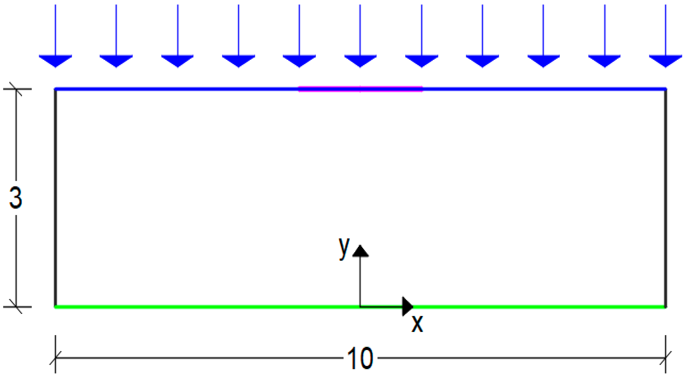
3.1. Setup of the Numerical Model

The implemented numerical model aims to reproduce migration through the vadose zone of an organic contaminant from a continuous source to the water table. The domain consists of a vertical column of soil, 10 m wide and 3 m high (Figure 1). As regards flow conditions, the initial distribution of pressure head is here assumed to be hydrostatic with the atmospheric pressure head at the water table; the top boundary condition is assumed to be of Neumann type—specifically, a constant or a transient inflow is set according to the selected precipitation scenario (blue arrows in Figure 1). At the initial time, the soil domain is assumed to be uncontaminated; therefore, the initial liquid phase concentration Cw (t = 0) is zero. A continuous source of contaminant with a concentration equal to 0.1 mg/L is placed on the ground surface. The contaminant is assumed to be non-volatile and non-reacting, and therefore, the degradation kinetic rate is equal to zero.
Meshing is performed by discretizing the computing domain in quadrilateral elements. Different mesh dimensions are tested, ranging from 0.1 to 0.03 m, to evaluate the convergence of the results. From the analysis, the dimension of 0.08 m is selected to achieve best accuracy while optimizing the computation time.

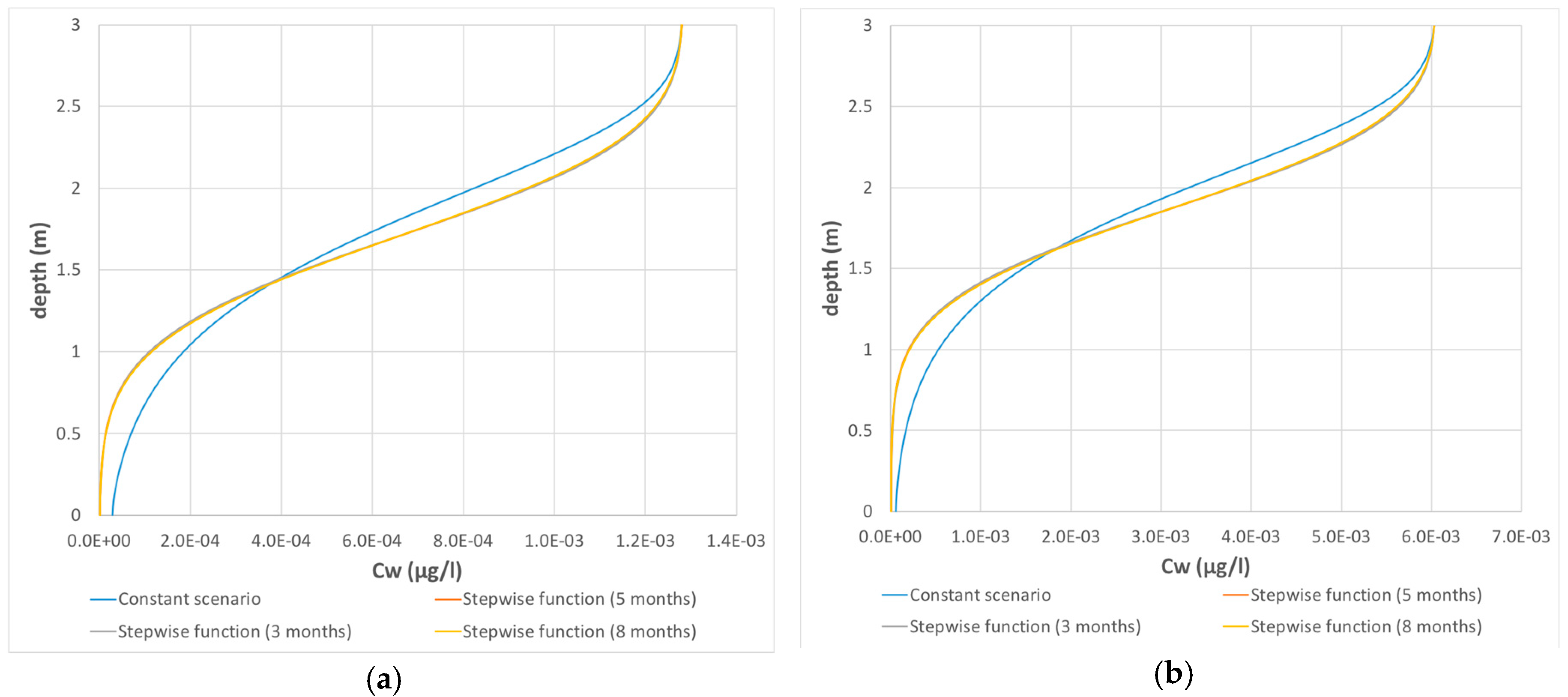
3.2. Comparison Methodology

Different simulations of contaminants transport are carried out concerning two substances with different physical behavior: benzene, a light non-aqueous liquid (LNAPL) belonging to aromatic hydrocarbons, and tetrachloroethylene (PCE), a dense non-aqueous liquid (DNAPL) falling within chlorinated solvents.
For each contaminant, four precipitation scenarios are set with a simulation period of two years. Keeping constant the annual effective infiltration as previously said, the infiltration is set in time according to two distributions: a non-varying, i.e., constant trend and a step-wise function where the annual precipitation is concentrated over a fixed period of time (Dt), shorter than a year, repeating itself periodically. Three Dt are taken into account: a three-, five-, and eight-month period, respectively. Data used for the analysis are taken from the pluviometric station of Gròmola, Campania Region, Italy.
Finally, the effects of the hydraulic conductivity and distribution coefficient on contaminant migration are evaluated considering three values of Ks [m/s], 10−6–10−5–10−4, and three values for Kd [m3/kg], 10−5–10−4–10−3. Each contaminant was then simulated for 36 cases, representing the different combinations of precipitation scenarios, hydraulic conductivity and distribution coefficient values, in order to assess the output effects as well as the sensitivity of the model to the variability of the input parameter.
The source concentration Cw0 is set equal to 100 µg/L for both the contaminants. Their physicochemical properties are derived from the database of the Italian National Institute of Health [27] and reported in Table 1.
The longitudinal dispersivity αl is calculated as a function of the travel distance, using the Gelhar relationship [28] (Equation (10))
l n α l = 4.933 + 3.811 l n z m z m 2
l n α l = 2.727 + 0.584 l n z m z m 2
where zm is the distance from the source to the observation location. In this case, zm is fixed equal to 3 m, and hence, αl is equal to 0.125. The transverse dispersivity is assumed to be a tenth of the longitudinal one, i.e., 0.0125.
A sandy loam soil, according to the United States Department of Agriculture (USDA) classification, is selected. The parameter values for this soil are derived from [29] and listed in Table 2.

4. Results and Discussion

In order to provide a first overview of the differences between the four precipitation scenarios, the values of Cw at a given time have been calculated as a function of the depth from the ground surface (Figure 2).
The 72 simulations exhibit similar trends: With the same distribution coefficient Kd, the two contaminants have similar concentration values, demonstrating the importance of these values with respect to others, such as the diffusion coefficient; the difference between steady and transient flow is significant, while the difference between the three transient distributions is not very pronounced. Furthermore, all the different contamination scenarios show the typical bell-shaped curve, and all curves intersect at the same point. As an example, in Figure 3 the graphs of the concentration on the 360th day with a Ks equal to 10−6 and Kd equal to 10−5 for benzene and tetrachloroethylene are reported.
Another comparison is developed between different distribution coefficient Kd, for the same contaminant and precipitation scenario. The analysis shows that contaminant concentration is significantly influenced by the variation of Kd. In Figure 3, the comparison between the benzene concentration obtained from the three values of Kd for a constant precipitation is shown. The graph shows that the contaminant travel distance after 360 days for a Kd value of 10−5–10−4–10−3 is about 0.6, 2.8, and more than 3 m, respectively.
For a better understanding of the migration trends, the values of Cw over time at three different depths (2, 1, and 0.5 b.g.s) are calculated. The graph concerning benzene concentration is reported in Figure 4.
The assessment of concentration over a time period of two years for the four precipitation scenarios (Figure 4) allowed us to obtain the following:
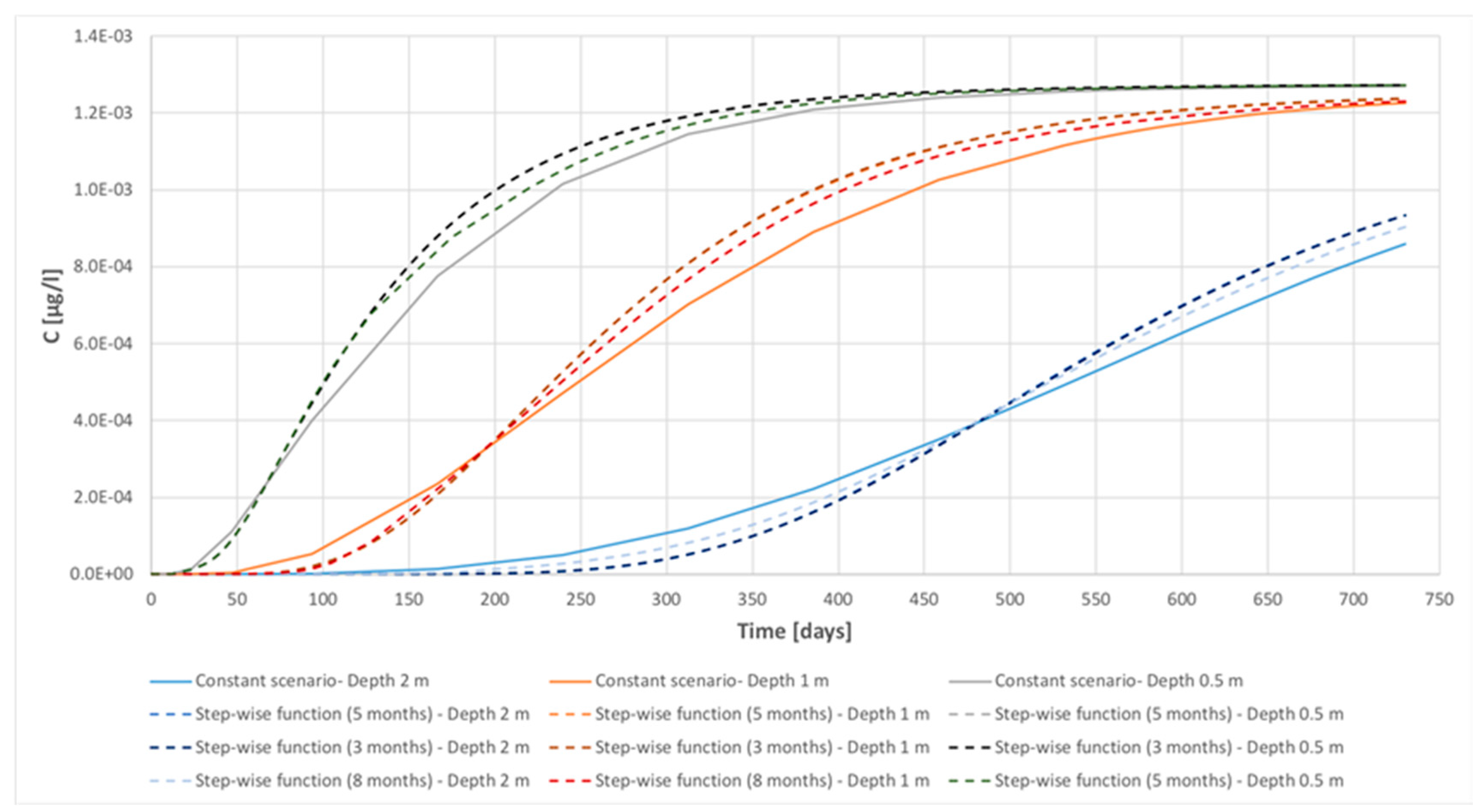
  • Three families of four curves each, the first one relating to the depth of 2 m in shades of blue, the second one relating to the depth of 1 m in shades of orange, and the third one relating to the depth of 0.5 m in shades of green. The i-th family (i = 1, …, 4) is related to the constant precipitation and the transient precipitation with a 3 months’ step, 5 months’ step, and 8 months’ step;
  • Each family of curves has the same inflexion point;
  • Curves follow a similar trend, with an initial concavity upwards and a final concavity downwards;
  • The effects of the different precipitation scenario are not predominant, compared to the remaining parameters being investigated.

5. Conclusions

A local and continuous spill of a contaminant on the ground surface of an unsaturated soil column was here investigated numerically. Thirty-six cases per contaminant (72 simulations in total) were run, representing different combinations of precipitation scenarios, hydraulic conductivity Ks values, and distribution coefficient Kd values. The aim was to assess the effects on the results of a steady or a transient infiltration flow as well as by changing Ks and Kd.
Three families, corresponding to depths z = 0.5, 1.0, and 2.0 m, of four curves (uniform infiltration and step-wise infiltration functions on 3, 5, and 8 months, respectively) were derived. It was observed that different precipitation scenarios did not have significant effects on the concentration outputs, probably because the stepwise function used in this study does not actually represent extreme infiltration events, which have major impacts on contaminant migration. Interestingly, each family of curves exhibited the same inflexion point in addition to a similar trend of the curves, with an initial concavity upwards and a final concavity downwards. The results show a significant effect of the distribution coefficient Kd on the modeled concentration and the travel distances, confirming that sorption phenomena have a key role in the fate and transport processes.

Author Contributions

G.V. and M.G.S. conceived and designed the experiments; S.L. performed the experiments; M.G.S. and S.L. analyzed the data; L.C. contributed to the conceptualization; G.V. and M.G.S. wrote the paper. All authors have read and agree to the published version of the manuscript.

Funding

This research received no external funding.

Conflicts of Interest

The authors declare no conflict of interest.

References

  1. Foster, S.; Hirata, R.; Gomes, D.; D’Elia, M.; Paris, M. Groundwater Quality Protection: A Guide for Water Service Companies, Municipal Authorities and Environment Agencies; The World Bank: Washington, DC, USA, 2002. [Google Scholar] [CrossRef]
  2. Withers, P.J.; Jordan, P.; May, L.; Jarvie, H.P.; Deal, N.E. Do septic tank systems pose a hidden threat to water quality? Front. Ecol. Environ. 2014, 12, 123–130. [Google Scholar] [CrossRef]
  3. Šimůnek, J.; van Genuchten, M.T. Contaminant transport in the unsaturated zone: Theory and modeling. In The Handbook of Groundwater Engineering, 3rd ed.; CRC Press: Boca Raton, FL, USA, 2016; pp. 221–254. ISBN 9781498703055. [Google Scholar]
  4. Rivett, M.O.; Wealthall, G.P.; Dearden, R.A.; McAlary, T.A. Review of unsaturated-zone transport and attenuation of volatile organic compound (VOC) plumes leached from shallow source zones. J. Contam. Hydrol. 2011, 123, 130–156. [Google Scholar] [CrossRef] [PubMed]
  5. Berlin, M.; Vasudevan, M.; Kumar, G.S.; Nambi, I.M. Numerical modelling on fate and transport of petroleum hydrocarbons in an unsaturated subsurface system for varying source scenario. J. Earth Syst. Sci. 2015, 124, 655–674. [Google Scholar] [CrossRef]
  6. Zhang, P.; Hu, L. Contaminant Transport in Soils Considering Preferential Flowpaths. Geoenviron. Eng. 2014, 50–59. [Google Scholar] [CrossRef]
  7. Pang, L.; Lafogler, M.; Knorr, B.; McGill, E.; Saunders, D.; Baumann, T.; Abraham, P.; Close, M. Influence of colloids on the attenuation and transport of phosphorus in alluvial gravel aquifer and vadose zone media. Sci. Total Environ. 2016, 550, 60–68. [Google Scholar] [CrossRef] [PubMed]
  8. Mulligan, C.N.; Yong, R.N. Natural attenuation of contaminated soils. Environ. Int. 2004, 30, 587–601. [Google Scholar] [CrossRef] [PubMed]
  9. Flury, M.; Wai, N.N. Dyes as tracers for vadose zone hydrology. Rev. Geophys. 2003, 41. [Google Scholar] [CrossRef]
  10. Vanderborght, J.; Vereecken, H. Review of dispersivities for transport modeling in soils. Vadose Zone J. 2007, 6, 29–52. [Google Scholar] [CrossRef]
  11. Goyne, K.W.; Jun, H.J.; Anderson, S.H.; Motavalli, P.P. Phosphorus and nitrogen sorption to soils in the presence of poultry litter-derived dissolved organic matter. J. Environ. Qual. 2008, 37, 154–163. [Google Scholar] [CrossRef] [PubMed]
  12. Kuntz, D.; Grathwohl, P. Comparison of steady-state and transient flow conditions on reactive transport of contaminants in the vadose soil zone. J. Hydrol. 2009, 369, 225–233. [Google Scholar] [CrossRef]
  13. Marshall, J.D.; Shimada, B.W.; Jaffe, P.R. Effect of temporal variability in infiltration on contaminant transport in the unsaturated zone. J. Contam. Hydrol. 2000, 46, 151–161. [Google Scholar] [CrossRef]
  14. Wang, P.; Quinlan, P.; Tartakovsky, D.M. Effects of spatio-temporal variability of precipitation on contaminant migration in the vadose zone. Geophys. Res. Lett. 2009, 36. [Google Scholar] [CrossRef]
  15. COMSOL Multiphysics®. v. 5.3. www.comsol.com; COMSOL AB: Stockholm, Sweden, 2020. [Google Scholar]
  16. Richards, L.A. Capillary conduction of liquids through porous mediums. Physics 1931, 1, 318–333. [Google Scholar] [CrossRef]
  17. Bear, J. Dynamics of Fluids in Porous Media; Courier Corporation: Chelmsford, MA, USA, 2013; ISBN 978-0486131801. [Google Scholar]
  18. Kosugi, K.; Hopmans, J.W.; Dane, J.H. Water retention and storage—parametric models. In Methods of Soil Analysis. Part. 4. Physical Methods; Dane, J.H., Topp, G.C., Eds.; Soil Science Society of America: Madison, WI, USA, 2002; pp. 739–758, ISBN 13 978-0891188414. [Google Scholar]
  19. Van Genuchten, M.T. A closed-form equation for predicting the hydraulic conductivity of unsaturated soils. Soil Sci. Soc. Am. J. 1980, 44, 892–898. [Google Scholar] [CrossRef]
  20. Song, X.; Yan, M.; Li, H. The development of a one-parameter model for the soil-water characteristic curve in the loess gully region. J. Food Agric. Environ. 2013, 11, 1546–1549. [Google Scholar] [CrossRef]
  21. Vanclooster, M.; Javaux, M.; Vanderborght, J. Solute transport in soil at the core and field scale. Encycl. Hydrol. Sci. 2006. [Google Scholar] [CrossRef]
  22. Bear, J.; Cheng, A.H.D. Modeling Groundwater Flow and Contaminant Transport (Volume 23); Springer Science and Business Media: Berlin, Germany, 2010; ISBN 978-1402066818. [Google Scholar]
  23. Foo, K.Y.; Hameed, B.H. Insights into the modeling of adsorption isotherm systems. Chem. Eng. J. 2010, 156, 2–10. [Google Scholar] [CrossRef]
  24. Brusseau, M.L.; Chorover, J. Chemical processes affecting contaminant transport and fate. In Environmental Pollution Science, 3rd ed.; Academic Press: Cambridge, MA, USA, 2019; Volume 8, pp. 113–130. [Google Scholar] [CrossRef]
  25. Allen-King, R.M.; Grathwohl, P.; Ball, W.P. New modeling paradigms for the sorption of hydrophobic organic chemicals to heterogeneous carbonaceous matter in soils, sediments, and rocks. Adv. Water Resour. 2002, 25, 985–1016. [Google Scholar] [CrossRef]
  26. Thornthwaite, C.W. An approach toward a rational classification of climate. Geogr. Rev. 1948, 38, 55–94. [Google Scholar] [CrossRef]
  27. ISS-ISPESL. Database of the Physico-Chemical and Toxicological Properties of Contamainants. Available online: http://old.iss.it/suol/?lang=1&id=96&tipo=13 (accessed on 22 May 2020). (In Italian).
  28. Gelhar, L.W. A Review of Field-Scale Physical Solute Transport Processes in Saturated and Unsaturated Porous Media; EA-4190, Research Project 2485-5; Electronic Power Research Institute: Palo Alto, CA, USA, 1985; 116p. [Google Scholar]
  29. Connor, J.A.; Newell, C.J.; Malander, M.W. Parameter estimation guidelines for risk-based corrective action (RBCA) modeling. In Proceedings of the Petroleum Hydrocarbons and Organic Chemicals in Groundwater Conference; National Ground Water Association: Houston, TX, USA; 1996; pp. 13–15. [Google Scholar]
Figure 1. Reference domain representing a soil portion. The contaminant source is set at y = 3 m.
Environsciproc 02 00034 g001
Figure 2. Concentration Cw at day 360 for different precipitation scenarios: (a) benzene; (b) tetrachloroethylene.
Environsciproc 02 00034 g002
Figure 3. Benzene concentration Cw at day 360 for different distribution coefficients.
Environsciproc 02 00034 g003
Figure 4. Benzene concentration Cw over time for different precipitation scenario.
Environsciproc 02 00034 g004
Table 1. Physical–chemical characteristics of the selected contaminants.
ParameterMeasurement UnitValues
BenzeneTetrachloroethylene
Molecular weightg/mol78.1165.8
Solubility (S)mg/L1750200
Diffusion coefficient in water (Dw)cm2/s9.80 × 10−68.20 × 10⁻⁶
Table 2. Soil parameter values.
ParameterMeasurement UnitValues
Soil bulk density (ρb)kg/m31700
Saturated water content (θs)-0.41
Residual water content (θr)-0.065
Van Genuchten parameter (α)-0.075
Van Genuchten parameter (n)-1.89
Publisher’s Note: MDPI stays neutral with regard to jurisdictional claims in published maps and institutional affiliations.

