An Interface Extension for the New EPANET 2.X †

1
Departamento de Informática, Universidade da Beira Interior, Rua Marquês d’Ávila e Bolama, 6201-001 Covilhã, Portugal
2
INESC Coimbra, DEEC, Universidade de Coimbra, Rua Sílvio Lima, Polo II 3030-290 Coimbra, Portugal
3
Instituto Politécnico de Castelo Branco, EST, U.T.C. Engenharia Civil, Av. do Empresário, 6000-767 Castelo Branco, Portugal
4
Departamento de Engenharia Civil, Instituto Politécnico de Coimbra, ISEC, Rua Pedro Nunes, 3030-199 Coimbra, Portugal
5
Instituto de Telecomunicações, Universidade da Beira Interior, Rua Marquês d’Ávila e Bolama, 6201-001 Covilhã, Portugal
6
Departamento de Engenharia Civil, Universidade de Coimbra, Rua Luís Reis Santos, Polo II, 3030-788 Coimbra, Portugal
*
Author to whom correspondence should be addressed.
†
Presented at the 4th EWaS International Conference: Valuing the Water, Carbon, Ecological Footprints of Human Activities, Online, 24–27 June 2020.
Environ. Sci. Proc. 2020, 2(1), 60; https://0-doi-org.brum.beds.ac.uk/10.3390/environsciproc2020002060
Published: 7 September 2020
(This article belongs to the Proceedings of The 4th EWaS International Conference: Valuing the Water, Carbon, Ecological Footprints of Human Activities)
Abstract
:The EPANET 2.0 is a public domain software used to model water distribution networks. The last main release dates to 2000. Recently, the Open Source EPANET Initiative has fixed some bugs and has brought new features to the EPANET solver, such as improved convergence or pressure-driven simulation, and has released it under a new version: EPANET 2.2. Although the legacy Graphical User Interface (GUI) still works with the updated Dynamic Link Library (DLL) (backward compatibility), it does not access the new features. This paper proposes and explores a GUI extension that takes advantage of the new pressure-driven features (such as pressure deficit or demand deficit). The paper also discusses some implementation aspects of the new solver that should be revisited in future releases.
1. Introduction
EPANET [1] is a Microsoft Windows program developed by the U.S. Environmental Protection Agency (USEPA) for hydraulic and quality simulation of drinking water distribution networks (WDN). The EPANET source-code was released as public domain and can be freely used and distributed. The tool itself is composed of two components: a Graphical User Interface (GUI) and a Dynamic Link Library (DLL). The GUI was developed in (Borland) Delphi, and the DLL (Programmer’s Toolkit) was coded in C language.
The last main release, EPANET 2.0, became available in 2000. Subsequent small fixes appeared in 2002 and 2008, under the builds 2.00.10 and 2.00.12, respectively. Recently (October 2018), the GUI was recompiled with (Embarcadero) Delphi 10 (build 2.00.12.01). The most recent official source code can be downloaded from the USEPA/EPANET web site [2].
Although the development of EPANET by USEPA ceased about 20 years ago, the tool continues to be used in the water industry world, by itself or incorporated in commercial software. EPANET is the de facto standard, being used to plan, design and analyze WDNs. However, the community claims for more modeling power, more numerical stability and more convergence control.
A major EPANET concern is when the nodal pressure is not enough to deliver the required demand because the simulation results are not physically accurate: EPANET was not designed for pressure-deficient scenarios. Some EPANET extensions address these issues, e.g., WaterNetGen [3,4,5], but in general, these extensions are black boxes where the source code is not available, and thus not auditable.
Recently, the Open Source EPANET Initiative [6,7] assumed the mission of further developing EPANET in an open source project. The latest developments can be found in a GitHub repository [8]. A first improved release, Version 2.1, appeared in July 2016, and more recently, December 2019, Version 2.2 appeared. These new DLLs are backward compatible, so the legacy GUI can work with the new and more stable solver. Another relevant change is that the new developments are now under the Massachusetts Institute of Technology (MIT) license.
Obviously, the legacy GUI cannot run pressure-driven simulations or access new convergence parameters and other user input-related enhancements. This paper proposes and explores a GUI extension that can take full advantage of the solver new features.
2. EPANET 2.2
The community focus has been on the EPANET solver. As previously stated, the current release (version 2.2) is backward compatible but includes several enhancements. The library itself can be built for Linux, Mac OS and Windows.
In version 2.2, it is possible to build a network model by code, just by calling API (Application Program Interface) functions, without the need to open an .inp file. Each network model is now linked with an internal object, that is, a project (handle). The API is extended with functions to create and delete projects and is thread-safe. To guarantee backward compatibility, the library also includes the legacy API functions that work over a default project.
Internally, a more efficient node reordering scheme is used, Multiple Minimum Degree (MMD) algorithm, instead of the Minimum Degree (MD) algorithm, to reduce the fill-in of the factorization of the sparse matrix that results from the linearization of the energy equations. The water quality module was rewritten to reduce/eliminate the mass balance errors, the handling of near-zero flows is improved, and additional convergence parameters were introduced to provide more rigorous convergence criteria for the hydraulic solver. It is possible to set the largest flow change (FLOWCHANGE) at any network element or the maximum head loss error (HEADERROR) that any network link can have. Additionally, some internal parameters (HTol, QTol and RQTol) are exposed to give augmented control on the convergence process.
The modeling capability is also extended: tanks can overflow and the demand can be pressure dependent. For the pressure-driven analysis (PDA), it is assumed that the available demand (qavl) is computed based on the following pressure-demand relationship [9]:
where Pref is the reference (or service) pressure necessary to fully satisfy the required demand qreq, Pmin is the pressure below which no water can be supplied, α (typically α = 0.5) is the exponent of the pressure-demand relationship, P is the current pressure. The parameters for the toolkit are the demand model (DEMAND MODEL, set to DDA or PDA), the minimum pressure (MINIMUM PRESSURE, Pmin), the required pressure (REQUIRED PRESSURE, Pref) and the pressure exponent (PRESSURE EXPONENT, α).
In scenarios of insufficient pressure, under PDA, it is possible to know the number of nodes that are pressure deficient, and the percentage and amount of demand reduction at the pressure deficient nodes.
3. GUI Extension
Two main ideas guided the process of building a GUI extension able to work with the new toolkit: adhesion to the open-source movement and keeping backward compatibility.
The first goal is pursued by hosting the source-code in a GitHub repository [10]. For the second goal, it was decided to use only the API without changing any toolkit function. In this way, new releases of the toolkit can be used without major concerns.
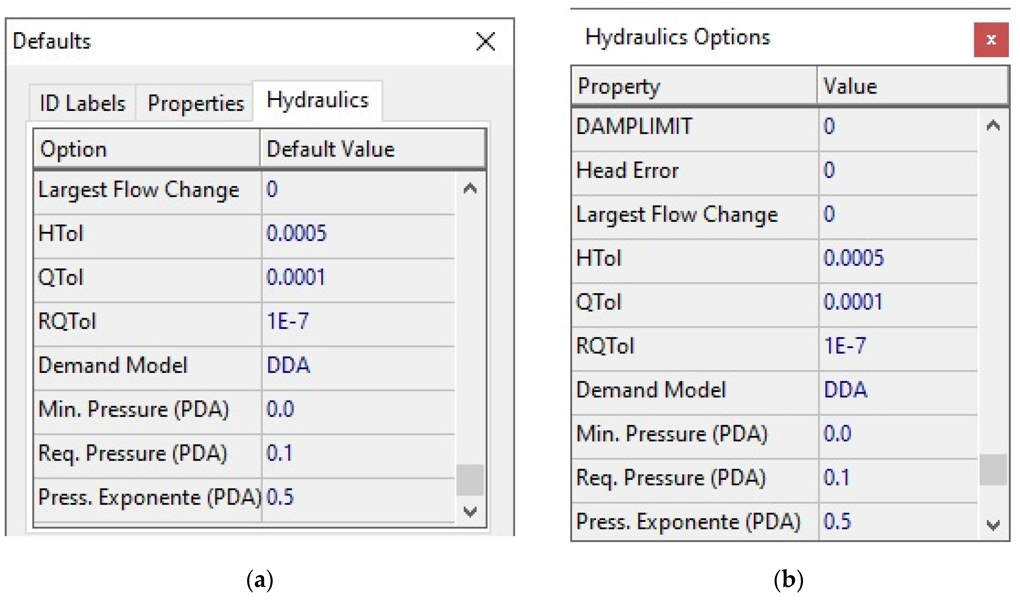
Convergence related parameters and PDA parameters are set in the Project | Defaults | Hydraulics page, or through the Hydraulics Options (from the Browser Data window)—Figure 1.
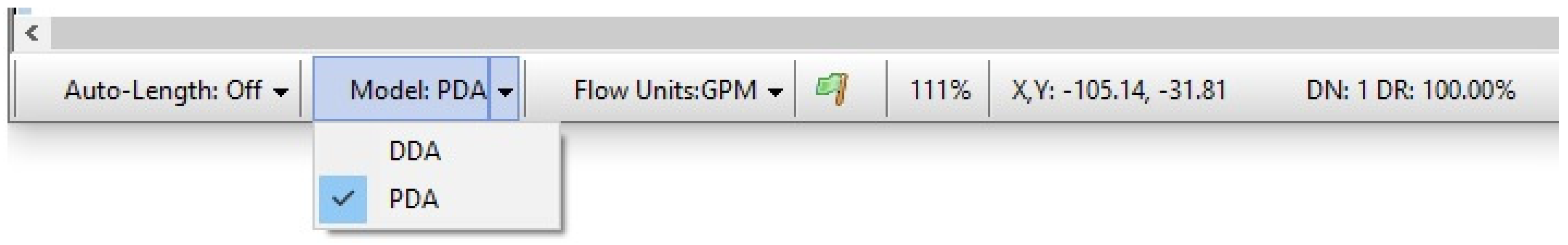
The demand model can be selected in the properties editor for the Hydraulics Options or in the Status Bar. The Status Bar also allows the change of the flow units and reports the number of pressure deficient nodes (DN) and their percentage of demand reduction (DR)—see Figure 2.
One of the most appreciated features of the EPANET user interface is its visualization capability with color-coded scales. Several output variables can be shown in the network map, for example, demand, pressure, head and chemical concentration, for nodes, and flow, velocity, unit head loss, for links. These output variables are computed by the solver at runtime and saved on a binary file for each time step. Due to questions related to backward compatibility, the number of variables (or its size) cannot be changed. Thus, the new pressure dependent data must be collected using the API and saved to a different binary file.
Accordingly, the RunHydraulics function was rewritten to collect and write data to a new file (for details see file Fsimul.pas in [10])—see Listing 1:
| Listing 1. The RunHydraulics function was rewritten to save pressure-dependent data to a binary file. |
| function TSimulationForm.RunHydraulics: Integer; begin ENopenH (); ENinitH ( 1 ); // Initialize hydraulics solver repeat // Solve hydraulics in each period ENrunH ( t ); ENnextH ( tstep ); // Get and save demand deficit values ENgetnodevalue (nodeIndex, EN_DEMANDDEFICIT, value) BlockWrite (F, DemandDefictArray, sizeof…); // Get and save number of pressure deficit nodes ENgetstatistic (EN_DEFICITNODES, value) BlockWrite (F, value, sizeof (single)); // Get and save demand reduction percent ENgetstatistic (EN_DEMANDREDUCTION, value) BlockWrite (F, value, sizeof (single)); until “no more steps” ENcloseH(); // Close hydraulics solver end; |
Two entries are added to the NodeVariable array (see Consts.txt in [10]), Pressure Deficit and Demand Deficit, and appended to the Browser Map window. In this way the user, at runtime, can easily find the nodes with pressure deficient conditions and their demand reduction. Like with other output variables, the user can build time series graphs and tables for these new variables.
The new parameters are saved in an EPANET-format input file, as expected by the EPANET toolkit. The GUI extension allows saving the network as an EPANET binary project file. The user can choose to save the network in the new format (v 2.2) or in the old one (v 2.0). In the latter case, the new parameters are lost.
4. Example
The EPANET example network Net2 was chosen to illustrate the PDA capabilities of the solver (release 2.2). For this purpose, the required pressure (Req. Pressure (PDA)) was set to 15 psi.
The simulation was run in the default demand-driven mode. The nodal pressures were enough, so all required demand was satisfied—see Figure 3.
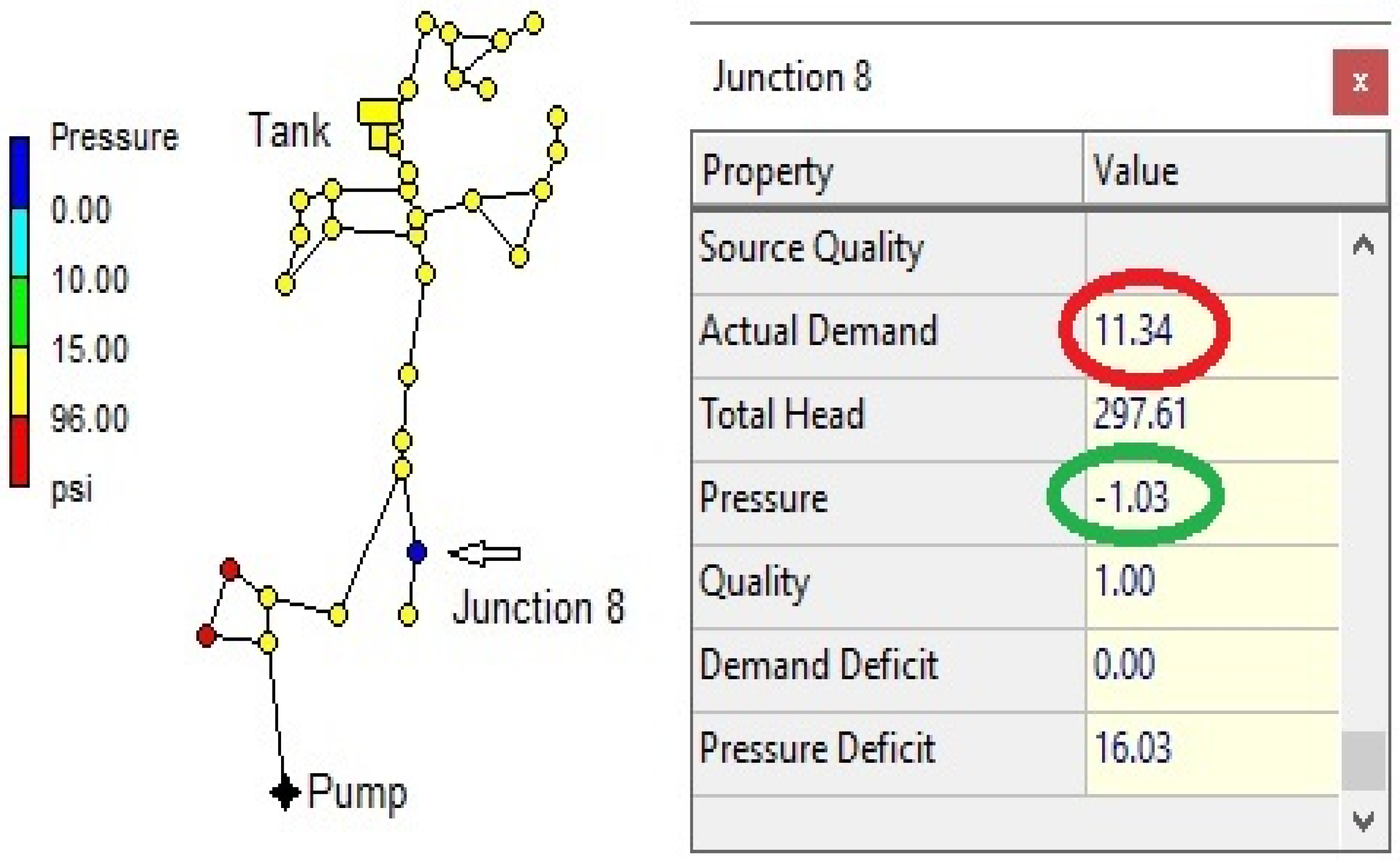
The next step was to induce a negative pressure in some node by changing its elevation. After changing junction 8 elevation, from 110 to 300 m, and running a new simulation, the program issued a warning message due to the presence of negative pressure.
The output variables for junction 8 showed a pressure of −1.03 psi and a total pressure deficit of 16.03 psi (=15 + 1.03)—see Figure 4.
Figure 4 also shows a physical impossibility: the required demand (11.34 GPM) was fully satisfied at a node that had negative pressure—this is a major concern of the demand-driven approach from EPANET.
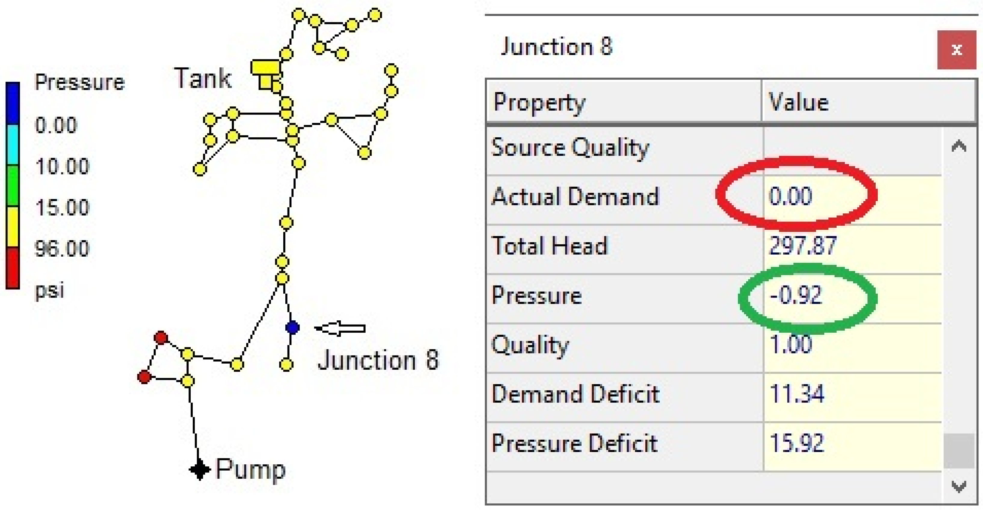
Selecting the pressure-driven approach (Demand Model set to PDA) and running again, the program ran successfully without any warning message. However, then, the Status Bar specified that there was one pressure deficient node with a demand reduction of 100% (DN: 1 DR: 100%).
Analyzing the program output, junction 8 still showed a negative pressure, but then, no demand was delivered. There existed a pressure deficit of 15.92 psi and a demand deficit of 11.34 GPM, which corresponded to a demand reduction of 100%—see Figure 5.
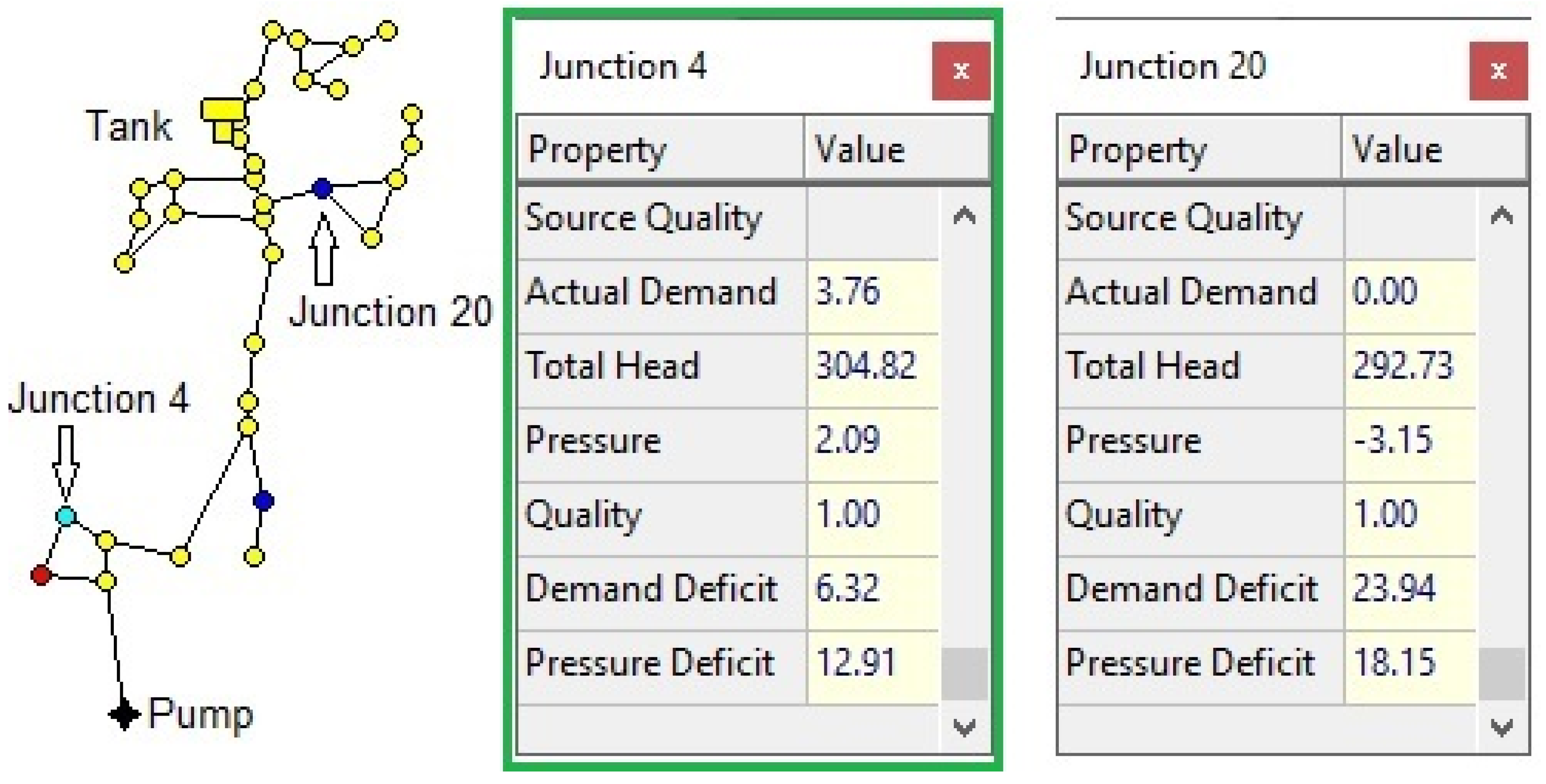
The scenario of pressure deficient conditions can be a little more severe, where several nodes do not have enough pressure to satisfy the required demand. Figure 6 shows a scenario where 3 nodes had their elevation set to 300 m. In this scenario, junctions 8 and 20 exhibited negative pressures, and junction 4 had a pressure that was greater than the minimum pressure but below the required pressure. The available demand for junction 4 was computed by expression (1) considering the actual pressure (2.09 psi) and the required demand (10.08 GPM). The Status Bar specified that, for this time step, there were 3 nodes with deficient pressure and a total demand reduction of 91.71% (DN: 3 DR: 91.71 %).
5. Discussion, Conclusions and Future Work
An EPANET GUI extension was developed to work together with the most recent release of the EPANET solver (DLL v2.2). The EPANET toolkit is not changed, so, at least in theory, the proposed extension is compatible with future releases of the toolkit. The new data are collected through API functions and handled on the GUI side of the tool.
It is shown how the new convergence parameters and PDA parameters are inserted in the graphical user interface and how the DLL and the GUI are set up to work together. The change from DDA to PDA and vice-versa is handled with just one mouse click, allowing a friendly user interaction.
The new pressure deficit and demand deficit variables, and its values, are integrated in the Browser Map, reducing in this way the user learning curve.
Regarding the solver current release (v2.2), there are some issues that should be revisited in future releases. Among these is the pressure-driven implementation. The use of global parameters for the minimum and required pressures does not allow the specification of networks with different pressure requirements and should be modified. Another issue that must be incorporated in the toolkit is the computation of leaks at pipe level, since it is closely related to the pressure-dependent behavior of the network. Besides these concerns, the new solver release is a big step in the right direction, and the proposed GUI extension follows it.
In the future, the authors plan to compare the solver results with their own implementation of the pressure-driven simulation (WaterNetGen) and study the behavior of the EPANET 2.2 solver when the current pressure approaches the minimum pressure, as it seems that the solver can face some convergence problems and numerical instabilities.
Author Contributions
All authors have read and agreed to the published version of the manuscript. The authors contributed equally to this work.
Funding
This research was partially funded by the Portuguese Foundation for Science and Technology under project UIDB/00308/2020.
Conflicts of Interest
The authors declare no conflict of interest.
References
- Rossman, L. EPANET 2 Users’ Manual; Risk Reduction Eng. Lab., Office of Research and Development, U.S. Environmental Protection Agency: Cincinnati, OH, USA, 2000. [Google Scholar]
- EPANET Web Site. 2020. Available online: https://www.epa.gov/water-research/epanet (accessed on 12 February 2020).
- Muranho, J.; Ferreira, A.; Sousa, J.; Gomes, A.; Sá Marques, A. WaterNetGen: An EPANET extension for automatic water distribution network models generation and pipe sizing. Water Supply 2012, 12, 117–123. [Google Scholar] [CrossRef]
- Muranho, J.; Ferreira, A.; Sousa, J.; Gomes, A.; Sá Marques, A. Pressure dependent demand and leakage modeling with an EPANET extension—WaterNetGen. Procedia Eng. 2014, 89, 642–639. [Google Scholar] [CrossRef]
- Muranho, J.; Ferreira, A.; Sousa, J.; Gomes, A.; Sá Marques, A. Convergence Issues in the EPANET solver. Procedia Eng. 2014, 119, 700–709. [Google Scholar] [CrossRef]
- Uber, J.; Boccelli, D.; Hatchett, S.; Kapelan, Z.; Saldarriaga, J.; Simpson, A.; Tryby, M.; van Zyl, J. Let’s Get Moving and Write Software: An Open Source Project for EPANET. J. Water Resour. Plan. Manag. 2018, 144, 01818001. [Google Scholar] [CrossRef]
- Salomons, E.; Hatchett, S.; Eliades, D. The EPANET Open Source Initiative. In Proceedings of the 1st International Joint Conference WDSA/CCWI, Kingston, ON, Canada, 23–25 July 2018. [Google Scholar]
- Open Water Analytics EPANET GitHub Site. 2020. Available online: https://github.com/OpenWaterAnalytics/EPANET (accessed on 12 February 2020).
- Wagner, J.M.; Shamir, U.; Marks, D.H. Water distribution reliability—Simulation methods. J. Water Res. Plan. Manag. 1988, 114, 276–294. [Google Scholar] [CrossRef]
- EPANET 2.2 Gui by WNG GitHub Site. 2020. Available online: https://github.com/WaterNetGen/Epanet-2.2-Gui-By-WNG (accessed on 12 February 2020).
Figure 1.
Properties editor for convergence related parameters and pressure-driven (PDA) parameters: (a) Project defaults settings; (b) Hydraulics Options.
Figure 1.
Properties editor for convergence related parameters and pressure-driven (PDA) parameters: (a) Project defaults settings; (b) Hydraulics Options.

Figure 2.
The Status Bar allows the selection of the demand model and the flow units, and informs about the number of deficient nodes (DN) and the percent of demand reduction (DR).
Figure 2.
The Status Bar allows the selection of the demand model and the flow units, and informs about the number of deficient nodes (DN) and the percent of demand reduction (DR).

Figure 3.
DDA: junction 8 had a pressure of 81.29 psi, so its demand was satisfied.

Figure 4.
DDA: junction 8 had a negative pressure (−1.03 psi), but apparently the demand was still satisfied.
Figure 4.
DDA: junction 8 had a negative pressure (−1.03 psi), but apparently the demand was still satisfied.

Figure 5.
PDA: junction 8 had a negative pressure (−0.92 psi) and no demand was delivered.

Figure 6.
PDA: junctions 8 and 20 had negative pressures, while although junction 4 had a positive pressure, it was not enough to fully satisfy the required demand.
Figure 6.
PDA: junctions 8 and 20 had negative pressures, while although junction 4 had a positive pressure, it was not enough to fully satisfy the required demand.

Figure 7.
PDA: pressure-deficient scenario: (a) pressure deficit; (b) demand deficit.

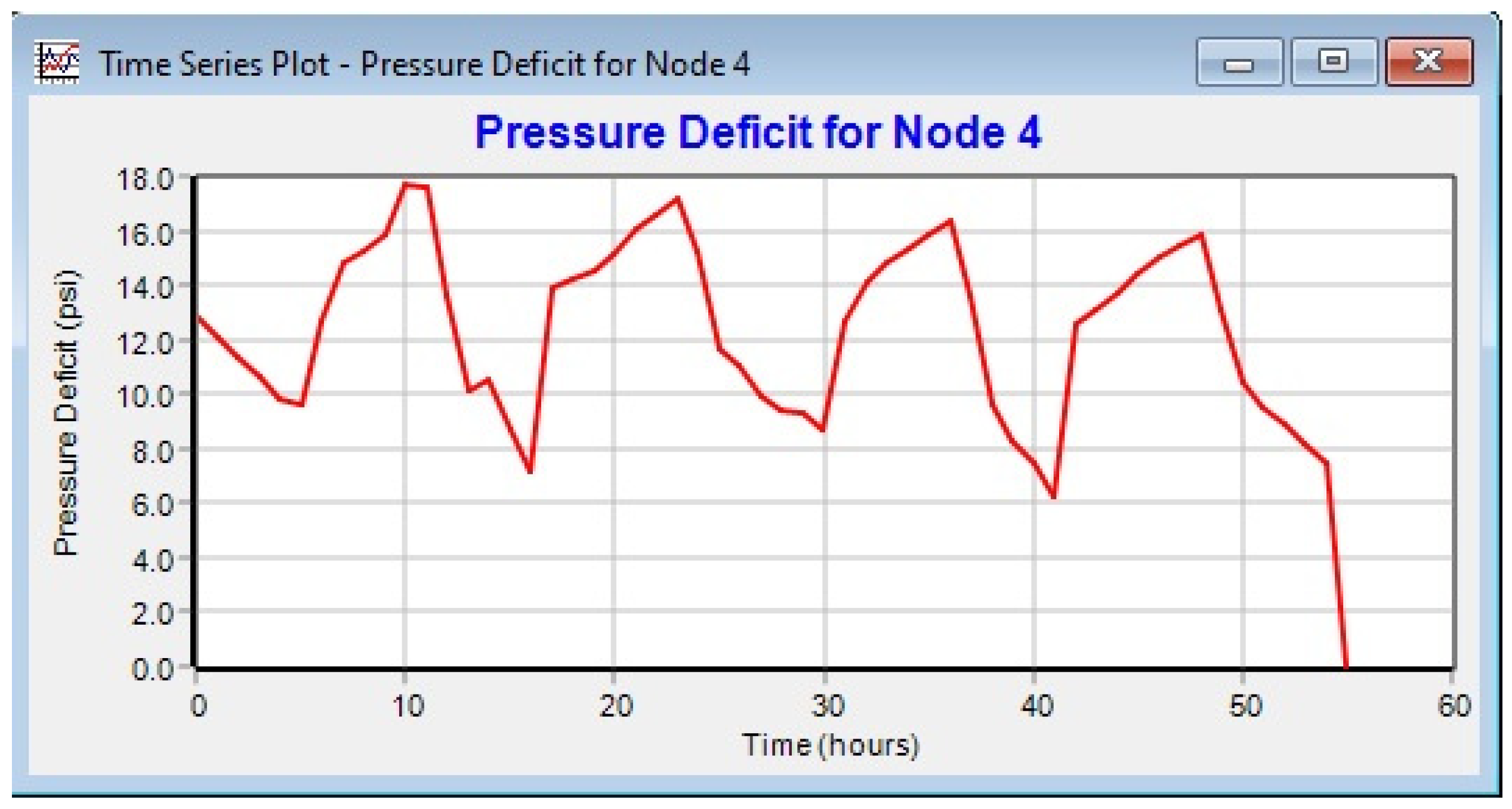
Figure 8.
PDA: pressure deficit for junction 4.

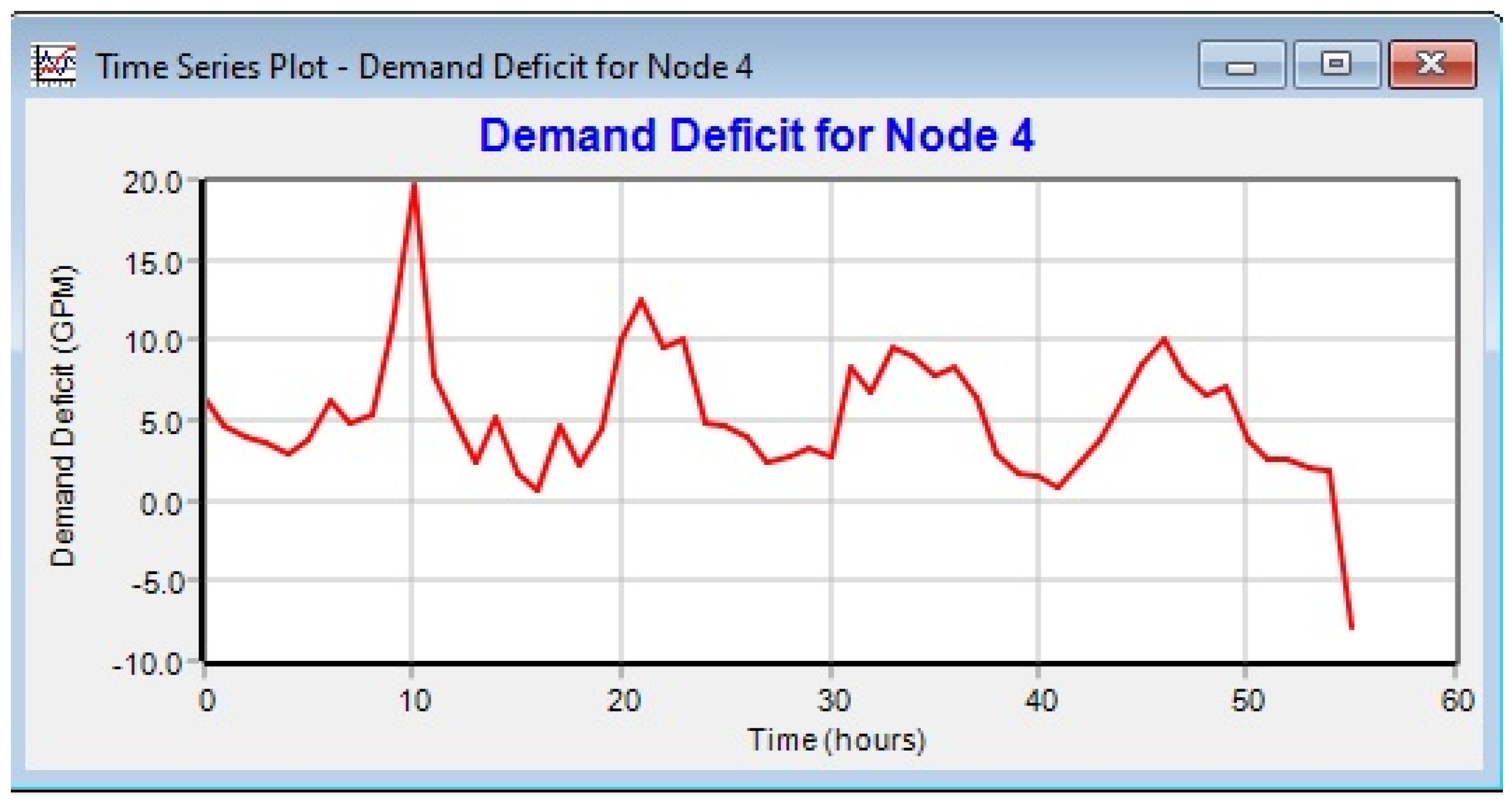
Figure 9.
PDA: demand deficit for junction 4.

Publisher’s Note: MDPI stays neutral with regard to jurisdictional claims in published maps and institutional affiliations. |
© 2020 by the authors. Licensee MDPI, Basel, Switzerland. This article is an open access article distributed under the terms and conditions of the Creative Commons Attribution (CC BY) license (https://creativecommons.org/licenses/by/4.0/).
Share and Cite
MDPI and ACS Style
Muranho, J.; Ferreira, A.; Sousa, J.; Gomes, A.; Marques, A.S. An Interface Extension for the New EPANET 2.X. Environ. Sci. Proc. 2020, 2, 60. https://0-doi-org.brum.beds.ac.uk/10.3390/environsciproc2020002060
AMA Style
Muranho J, Ferreira A, Sousa J, Gomes A, Marques AS. An Interface Extension for the New EPANET 2.X. Environmental Sciences Proceedings. 2020; 2(1):60. https://0-doi-org.brum.beds.ac.uk/10.3390/environsciproc2020002060
Chicago/Turabian StyleMuranho, João, Ana Ferreira, Joaquim Sousa, Abel Gomes, and Alfeu Sá Marques. 2020. "An Interface Extension for the New EPANET 2.X" Environmental Sciences Proceedings 2, no. 1: 60. https://0-doi-org.brum.beds.ac.uk/10.3390/environsciproc2020002060