
Evaluation of a Meta-Analysis of Ambient Air Quality as a Risk Factor for Asthma Exacerbation


1
School of Public Health, University of Alberta, Edmonton, AB T6G 1C9, Canada
2
CGStat, Raleigh, NC 27607, USA
3
Outcome Based Medicine, Raleigh, NC 27614, USA
4
401 Rocky Hill Road, Brownwood, TX 76801-0986, USA
*
Author to whom correspondence should be addressed.
J. Respir. 2021, 1(3), 173-196; https://0-doi-org.brum.beds.ac.uk/10.3390/jor1030017
Submission received: 29 April 2021
/
Revised: 10 June 2021
/
Accepted: 16 June 2021
/
Published: 25 June 2021
Abstract
:Background: An irreproducibility crisis currently afflicts a wide range of scientific disciplines, including public health and biomedical science. A study was undertaken to assess the reliability of a meta-analysis examining whether air quality components (carbon monoxide, particulate matter 10 µm and 2.5 µm (PM10 and PM2.5), sulfur dioxide, nitrogen dioxide and ozone) are risk factors for asthma exacerbation. Methods: The number of statistical tests and models were counted in 17 randomly selected base papers from 87 used in the meta-analysis. Confidence intervals from all 87 base papers were converted to p-values. p-value plots for each air component were constructed to evaluate the effect heterogeneity of the p-values. Results: The number of statistical tests possible in the 17 selected base papers was large, median = 15,360 (interquartile range = 1536–40,960), in comparison to results presented. Each p-value plot showed a two-component mixture with small p-values < 0.001 while other p-values appeared random (p-values > 0.05). Given potentially large numbers of statistical tests conducted in the 17 selected base papers, p-hacking cannot be ruled out as explanations for small p-values. Conclusions: Our interpretation of the meta-analysis is that random p-values indicating null associations are more plausible and the meta-analysis is unlikely to replicate in the absence of bias.
1. Introduction
One aspect of replication—the performance of another study statistically confirming the same hypothesis or claim—is a cornerstone of science and replication of research findings is particularly important before causal inference can be made [1]. However, an irreproducibility crisis currently afflicts a wide range of scientific disciplines, including public health and biomedical science. Far too frequently, scientists are unable to replicate claims made in published research [2].
A branch of biomedical science—environmental epidemiology—depends, in part, on establishing statistical associations in default of establishing direct causal biological links between risk factors and health outcomes such as respiratory diseases (e.g., asthma, chronic obstructive pulmonary disease). We have previously shown through independent analysis that published environmental epidemiology studies claiming air quality–heart attack associations may be compromised by false-positives and bias [3,4]. For the present study we examined whether these shortcomings are occurring with observational studies of air quality–asthma attack associations.
1.1. False-Positives and Bias in Biomedical Science Literature
False-positives—False-positive results may be a common feature of the biomedical science literature with others estimating that a large portion of positive (statistically significant) research findings that physicians rely on—as much as 90 percent—may be flawed [5] and simply ‘false-positives’ [6]. Today the traditional 0.05 p-value has lost its ability to discriminate important biomedical science research findings, especially when numerous comparisons (multiple tests) are being made, and can produce research results that are irreproducible and, in some examples, harmful to the public’s health [7].
False-positive findings can arise in research when statistical methods are applied incorrectly or when p-values (or confidence intervals) are interpreted without sufficient understanding of the multiple testing problem [8]. False-positive results are reported to dominate the epidemiologic literature, with most of the traditional areas of epidemiologic research more closely reflecting the performance settings and practices of early human genome epidemiology showing at least 20 false-positive results for every one true-positive result [9]. On the other hand, studies with negative (non-statistically significant) results are more likely to remain unpublished than studies with positive results [10]. Epidemiological literature may be distorted as a result and any systematic reviews or meta-analyses of these studies would be biased [11,12] because they are summarizing information and data from a misleading, selected body of evidence [13,14,15]. Too many of the results coming from observational studies turn out to be wrong when they are re-examined [16]. This excess of false-positive results in published observational (and experimental) literature has been attributed mostly to bias [17,18,19,20,21].
Bias—Bias consists of systematic alteration of research findings due to factors related to study design, data acquisition, analysis or reporting of results [18]. Selective reporting proliferates in published observational studies where researchers routinely test many models and questions during a study and then report those models that offer interesting (statistically significant) results [22]. Selective reporting biases affecting overall results and specific analyses within studies are reported by others to likely be the greatest and most elusive issue distorting published research findings in the biomedical science field today [23,24,25,26,27].
There are at least 235 catalogued biases in published biomedical science literature [28]. Although most of the listed terminology for bias in literature is used infrequently, different bias terms used in diverse disciplines appear to refer to biases that have overlapping/similar meaning. Some of the more common bias terms used in current biomedical science literature include [28]: publication bias, confounding, selection bias and response bias. These types of biases may be important in observational studies of air quality–asthma attack associations. Published observational studies exists that question or do not find air quality–asthma attack associations [29,30,31,32,33].
1.2. Positive and Negative Predictive Values of Risk Factor–Chronic Disease Effects
Because of the prominence of disease prevention in our current health care system, observational risk factor–chronic disease research plays a key role in providing evidence to public health decision makers; e.g., providing advice on the intervention of asthma. Analysis of biomedical diagnostic test results being true depends on sensitivity, specificity and disease prevalence in a population [34,35,36]. Similar to this, a Bayesian simulation model was developed to quantify the extent of non-replicability in a study (i.e., the number of research results in a study that are expected to be “false”) [37]. This theoretical model relies on statistical hypothesis testing, incorporating pre-study (i.e., prior) odds of a research result being true, the number of statistical significance tests, a quantitative measure of investigator bias and other factors. The model can be used to understand the probability of a research finding in a single study being true in the presence of bias.
Others have critiqued the model and noted [38]: many biomedical science research findings are less definitive than readers suspect, p-values are widely misinterpreted, bias of various forms is widespread, multiple approaches are needed to prevent the literature from being systematically biased, and there is a need for more data on the prevalence of false claims. The National Academy of Science, Engineering and Medicine stated that [14]… any initial results that are statistically significant [in a study] need further confirmation and validation. These positions support a need for independent testing of statistically significant (positive) research claims made in published biomedical science literature.
Given the importance of bias in observational studies [39], we extended the simulation model to estimate the probability of positive research findings (Positive Predictive Value or PPV) and negative, or null, research findings (Negative Predictive Value or NPV) in a single study being true for different levels of bias and prevalence rates for asthma and the other most common chronic diseases in United States. Table 1 presents estimates of prevalence for the most common chronic diseases of interest in United States (Supplemental Information (SI) 1 provides details upon which estimates are based). The four most common types of chronic diseases in the world’s population (including developed and developing countries) are [40,41]: respiratory diseases (primarily asthma), heart and stroke disease, diabetes and cancers.
Using relationships we developed in SI 1, Figure 1 illustrates the theoretical probability of a research finding in a single study being true as a function of disease prevalence within the range 0.0001 to 0.1. In Figure 1 we show how bias affects the probability for two situations: a study collectively influenced by relatively minor biases (0.2), and a study collectively influenced by relatively major biases (0.8).
Bias represents the proportion of probed analyses [relationships] in a study that would not have been “research findings,” but nevertheless end up presented and reported as such, because of bias [37]. This definition does not distinguish among different ways researchers can alter findings due to factors related to study design, data acquisition, analysis or reporting of results, etc. It simply aggregates these forms of bias into a single quantity ranging between 0 and 1. Figure 1 suggests that asthma and other most common chronic diseases listed in Table 1 correspond with low post-study probabilities of a positive research finding in a study being true—less than 30%. On the other hand, these diseases correspond with high post-study probabilities of a negative (null) research finding in a study being true—greater than 95%.
Figure 1 suggests that for asthma and the other common chronic diseases of interest—i.e., diseases with a prevalence < 0.1—NPV (PPV) has relatively small (large) dependence on prevalence and bias. Figure 1 also suggests that a PPV exceeding 30% is difficult to achieve in risk factor–chronic disease epidemiological research for asthma and the other most common chronic diseases of interest. A majority of modern biomedical science research making positive claims may be operating in areas with very low pre- and post-study probability for true findings [37], including asthma and other chronic diseases listed in Table 1. This, in part, may help explain why false-positive results dominate the epidemiologic literature in this area. This is consistent with others [9] reporting that most traditional fields of epidemiologic research have high ratios of false-positive to false-negative findings. It is also consistent with the general claim that false-positive results are common features of the biomedical science literature today, including the broad range of risk factor–chronic disease research [42,43,44].
1.3. Ambient Air Quality–Chronic Disease Observational Studies
Many published observational epidemiology studies claim certain air quality components are risk factors that are causal of chronic diseases [45,46,47]. Claims that ambient air quality causes all the diseases listed in Table 1 have been made using meta-analysis—asthma [48], COPD [49], heart attack [50], diabetes [51], and breast [52], prostate [53], colorectal [54] and lung cancer [55]. However, it has been noted that, in the presence of unmeasured confounders, causality is hard to establish for a relatively weak health risk factor such as ambient air quality [56]. Low post-study probabilities for asthma and the other common chronic diseases (see Table 1 and Figure 1) may offer statistical reasons to question the reliability of these claims.
Part of this ‘reliability’ problem may arise from researchers of modern ambient air quality–health effect observational studies performing large numbers of statistical tests and using multiple statistical models—referred to as MTMM (multiple testing and multiple modelling) [4,42,57,58]:
- Multiple testing involves statistical null hypothesis testing of many separate predictor (e.g., air quality) variables against numerous representations of dependent (e.g., chronic disease) variables taking into account covariates, which may or may not act as confounders. For example, different air quality predictor variables—nitrogen dioxide, carbon monoxide—can be tested in the presence/absence of weather variables (e.g., temperature, relative humidity, etc.) against effects (e.g., heart attack hospitalizations) in a whole population of interest, females only, males only, those greater than 55 years old, etc.
- Multiple modelling involves testing using multiple Model Selection procedures or different model forms (e.g., simple univariate, bivariate or multivariate logistic regression, etc.). For example, different models can be used in a single study to test independent predictor variables and covariates against dependent (e.g., chronic disease) variables.
MTMM is analogous to what others call Model Selection in statistical models used to estimate the effects of environmental impacts [59,60]. This refers to the fact that with k potential explanatory variables in a model one can in principle run 2k possible regressions and select one after the fact that that yields the ‘best’ or ‘most interesting’ result. p-Hacking is multiple testing and multiple modelling without statistical correction [61,62,63,64]. It involves the relentless search for statistical significance and comes in many forms [65]. It enables researchers to find statistically significant results even when their samples are much too small to reliably detect the effect they are studying or even when they are studying an effect that is non-existent [66]. Examples of different forms of p-hacking include [67]: increasing sample size, analyzing data subsets, increasing variables in a model, adjusting data, transforming data (i.e., log transformations), removing suspicious outliers, changing the control group, using different statistical tests.
1.4. Objective of the Current Study
We have previously reported on the potential for epidemiology literature, particularly observational studies related to air quality component–heart attack associations, to be compromised by false-positives and bias [3,4]. For the present study we were interested in exploring whether the same sort of issues might be occurring with observational studies of air quality component–asthma attack associations. Asthma has an estimated prevalence in United States of 0.079 (Table 1) with any ambient air quality–chronic disease observational study ‘positive effect’ having a low theoretical post-study probability of being true—less than 25% (Figure 1).
A meta-analysis offers a window into a research claim, for example, that some ambient air quality components are causal of a chronic disease. A meta-analysis examines a claim by taking a summary statistic along with a measure of its reliability from multiple individual ambient air quality–chronic disease studies (base papers) found in the epidemiological literature. These statistics are combined to give what is supposed to be a more reliable estimate of an air quality effect. A key assumption of a meta-analysis is that estimates drawn from the base papers for the analysis are unbiased estimates of the effect of interest [68]. However, as stated previously, studies with negative results are more likely to remain unpublished than studies with positive results leading to distortion of effects in the epidemiological literature and subsequent unreliable meta-analysis of these effects [10,11,12,13,14,15].
Here, we evaluated the meta-analysis study of Zheng et al. [48]. This meta-analysis has received 280 Google Scholar citations as of 21 April 2021. We were interested in evaluating two specific properties of the meta-analysis following along the lines of two recent published studies [3,4]:
- Whether heterogeneity across the base papers of the meta-analysis is more complex than simple sampling from a single normal process [69].
2. Methods
Zheng et al. [48] undertook a systematic computerized search of published observational studies to identify those studies focusing on short-term exposures (same day and lags up to 7 days, which are never chosen a priori) to six ambient air quality components—carbon monoxide (CO), particulate matter with aerodynamic equivalent diameter ≤10 micron (PM10), particulate matter with aerodynamic equivalent diameter ≤2.5 micron (PM2.5), sulfur dioxide (SO2), nitrogen dioxide (NO2) and ozone (O3)—and asthma exacerbation (hospital admission and emergency room visits for asthma attack).
Associations between air quality components and asthma-related hospital admission and emergency room visits were expressed as risk ratios (RRs) and 95% confidence intervals (CIs) that were derived from single-pollutant models reporting RRs (95% CIs) or percentage change (95% CIs). They further recalculated these associations to represent a 10 μg/m3 increase, except for CO (where they recalculated associations to represent a 1 mg/m3 increase). Zheng et al. [48] concluded that all six air quality components were associated with significantly increased risks of asthma-related hospital admission and emergency room visits for all air quality components:
- CO: RR (relative risk) = 1.045 (95% CI (confidence interval) 1.029, 1.061);
- PM10: RR = 1.010 (95% CI 1.008, 1.013);
- PM2.5: RR = 1.023 (95% CI 1.015, 1.031);
- SO2: RR = 1.011 (95% CI 95% CI 1.007, 1.015);
- NO2: RR = 1.018 (95% CI 1.014, 1.022);
- O3: RR = 1.009 (95% CI 1.006, 1.011).
It is generally accepted that there are two classes of causes of asthma—primary and secondary [70]. ‘Primary’ causes of asthma relate to the increase in risk of developing the disorder (e.g., asthma). Whereas ‘secondary’ causes relate to triggering/precipitation of asthma exacerbation. The Zheng et al. meta-analysis focused studies of short-term exposures to ambient air quality components and hence on secondary causes of asthma. Zheng et al. initially identified 1099 literature reports. After screening titles and abstracts of these reports, they selected and assessed 246 full-text articles for eligibility, of which 87 base papers were selected for their meta-analysis. Citations and summary details for the 87 base papers each used by Zheng et al. in their meta-analysis are provided in SI 2.
2.1. Analysis Search Space
Analysis search space (or search space counts) represents an estimate of the number of exposure-disease combinations tested in an observational study. Our interest in search space counts is explained further. During a study there is flexibility available to researchers to undertake a range of statistical tests and use different statistical models (i.e., perform MTMM) before selecting, using and reporting only a portion of the test and model results. This researcher flexibility is commonly referred to as researcher degrees of freedom in the psychological sciences [71].
Base papers with large search space counts suggest the use of large numbers of statistical tests and statistical models and the potential for researchers to search through and only report only a portion of their results (i.e., results showing positive, statistically significant results). As acknowledged elsewhere [4], search space counts are considered lower bound approximations of the number of tests possible.
A 5–20% sample from a population whose characteristics are known is considered acceptable for most research purposes as it provides an ability to make generalizations for the population [72]. Given the prior screening and data collection procedures used by Zheng et al., we assumed that their 87 papers had sufficiently consistent characteristics suitable for use in meta-analysis. Based on this assumption, we randomly selected 17 of the 87 papers (~20%) for search space counting in the following manner. Using methods described previously [3,4,73], we started with the 87 base papers and assigned a separate number in ascending order to each paper (numbered 1–87). We then used the online web tool numbergenerator.org to generate 10 random numbers between 1 and 87. We then removed the 10 selected papers from the ordered list, renumbered the remaining papers 1–77 and used the web tool to generate another 7 random numbers between 1 and 77. This allowed us to select 17 of the Zheng et al. base papers for further evaluation (refer to SI 2).
Electronic copies of the 17 randomly selected base papers (and any corresponding electronic Supplementary Information Files) were obtained and read. One change was made from previous search space counting procedures we used [3,4]. It was apparent that several of the base papers we selected [74,75,76,77] employed a variety of model forms in their analysis. To accommodate this, we separately counted the number of model forms along with the number of outcomes, predictors, time lags, covariates reported in each base paper (covariates can be vague as they might be mentioned anywhere in a base paper). Specifically, analysis search space of a base paper was estimated as follows:
- The product of outcomes, predictors, model forms and time lags = number of questions at issue, Space1.
- A covariate may or may not act as a confounder to a predictor variable and the only way to test for this is to include/exclude the covariate from a model. As it can be in or out of a model, one way to approximate the modelling options is to raise 2 to the power of the number of covariates, Space2.
- The product of Space1 and Space2 = an approximation of analysis search space, Space3.
Table 2 provides three examples of search space analysis of a hypothetical observational study of ambient air quality versus hospitalization due to asthma exacerbation.
2.2. p-Value Plots
It is traditional in epidemiology to use confidence intervals instead of p-values from a hypothesis test to demonstrate or interpret statistical significance. As both confidence intervals and p-values are constructed from the same data, they are interchangeable, and one can be calculated from the other [78,79]. We first calculated p-values from confidence intervals for data from the Zheng et al. meta-analysis. Following the ideas of others [80], p-value plots were then developed to inspect the distribution of the set of p-values reported for each ambient air quality component.
The p-value can be defined as the probability, if nothing is going on, of obtaining a result equal to or more extreme than what was observed. The p-value is a random variable derived from a distribution of the test statistic used to analyze data and to test a null hypothesis. The p-value is distributed uniformly over the interval 0 to 1 regardless of sample size under the null hypothesis and a distribution of true null hypothesis points in a p-value plot should form a straight line [80,81].
A plot of p-values sorted by rank corresponding to a true null hypothesis should conform to a near 45-degree line. The plot can be used to assess the validity of a false claim being taken as true and, specific to our interest, can be used to examine the reliability of base papers used in the Zheng et al. meta-analysis.
p-Value plots for each ambient air quality component were constructed and interpreted as follows [80]:
- p-Values were computed using the method of others [79] and ordered from smallest to largest and plotted against the integers, 1, 2, 3, …
- If the points on the plot follow an approximate 45-degree line, then the p-values are assumed to be from a random (chance) process—supporting the null hypothesis of no significant association.
- If the points on the plot follow approximately a line with slope < 1, where most of the p-values are small (less than 0.05), then the p-values provide evidence for a real effect—supporting a statistically significant association.
- If the points on the plot exhibit a bilinear shape (divide into two lines), then the p-values used for meta-analysis constitute a mixture and a general (over-all) claim is not supported; in addition, the p-value reported for the overall claim in the meta-analysis paper cannot be taken as valid.
To assist interpretation of the p-value plots we constructed, we also show p-value plots for plausible true null outcomes (supporting the null hypothesis of no significant association) and true alternative hypothesis outcomes (supporting a statistically significant association) based on meta-analysis of observational datasets.
3. Results
3.1. Analysis Search Space
Estimated analysis search spaces for the 17 randomly selected base papers from Zheng et al. are presented in Table 3. From Table 3, investigating multiple (i.e., 2 or more) asthma outcomes in the selected base were as common as single outcome investigations. In addition, use of multiple models and lags was common in their analysis, so were adjustments for multiple possible covariate confounders. While the use of multiple factors (i.e., outcomes, predictors, models, lags and treatment of covariates) is seemingly realistic, these attempts to find possible exposure–disease associations among combinations of these factors will increase the overall number of statistical tests performed in a single study (e.g., refer to Table 2).
Summary statistics of the possible numbers of tests in the 17 base papers are presented in Table 4. The median number of possible statistical tests (Space3) of the 17 randomly selected base papers was 15,360 (interquartile range 1536–40,960), in comparison to actual statistical test results presented. Given these large numbers, statistical test results taken from the base papers are unlikely to provide unbiased measures of effect for meta-analysis.
3.2. p-Values
The method we used for calculating p-values [79] recommends reporting 0.0001 for a calculated p-value smaller than 0.0001. Consequently, p-values calculated < 0.0001 were reported simply as 0.0001. This was done to facilitate creation of p-value plots for each air quality component. Zheng et al. drew upon many (332) summary statistics from 87 base papers for their meta-analysis of six air quality components. Summary statistics they used in their meta-analysis of PM2.5 (i.e., Risk Ratio (RR), Lower Confidence Level (LCL) and Upper Confidence Level (UCL) values) and p-values we calculated are presented in Table 5. Summary statistics for the other air quality components (CO, NO2, O3, SO2 and PM10) and calculated p-values are provided in SI 3. In Table 5 (and tables presented in SI 3), calculated p-values ≤ 0.05, taken as a statistically significant result, are bolded and italicized.
Table 6 presents additional information on each of the air quality components (i.e., RR and p-value counts). Zheng et al. drew upon 37 summary statistics from 32 base papers for their PM2.5 meta-analysis. The majority of PM2.5 summary statistics had p-values greater than 0.05 (22 of 37), 15 of 37 were smaller than 0.05 and 8 of 37 were smaller than 0.001. Researchers often accept a p-value of 0.001 or smaller as virtual certainty [4]. If a summary statistic has a p-value small enough to indicate certainty, one should expect few p-values larger than 0.05 [68,82]. This is not the case as 45% or more of all summary statistics used by Zheng et al. had p-values greater than 0.05 (refer to Table 6).
Epidemiological literature can be distorted, i.e., mostly containing studies with positive results, and any meta-analysis of these studies are summarizing information and data from a misleading body of evidence [11,12,13,14,15]. Yet, even with this prevailing bias and given the base studies selected by Zheng et al., their many null results in Table 6 for each air quality component (third column) are not encouraging support for an effect.
3.3. p-Value Plots
A plot of ranked p-values versus integers for a dataset of a true null relationship would present as a sloped line going left to right at approximately 45-degrees. Whereas a plot of ranked p-values versus integers for a dataset of a plausible true relationship should have a majority of p-values smaller than 0.05. To support this, p-value plots of small datasets (n < 13 base papers) taken from a meta-analysis of selected cancers in petroleum refinery workers [83] are presented in SI 4. The distribution of the p-value under the alternative hypothesis—where the p-value is a measure of evidence against the null hypothesis—is a function of both sample size and the true value or range of true values of the tested parameter [81].
The p-value plots shown in SI 4 conform to that explained above—i.e., sloped line from left to right at an approximate 45-degrees for data suggesting a plausible true null chronic myeloid leukemia causal relationship in petroleum refinery workers and a majority of p-values below the 0.05 line for data suggesting a plausible true mesothelioma causal relationship in petroleum refinery workers. Another set of p-value plots of meta-analysis datasets for large numbers of base papers (n > 65) are illustrated in SI 5 (true null relationship [84]) and SI 6 (true relationship [85]).
Figure 2 presents p-value plots for each of the six air components in the Zheng et al. meta-analysis. All these plots are different from p-value plot behavior of both plausible true null and true relationships (refer to p-value plots in SI 4–SI 6). Variability among data is apparent in p-value plots for each air component. For example, the p-value plot for PM2.5 (lower left image) presents as a distinct bilinear (two-component) mixture. This two-component mixture may suggest a true-positive causal relationship or a false-positive causal relationship due to p-hacking for p-values below the 0.05 line, and random outcomes or false-negative relationships for p-values above the 0.05 line.
p-Value plots are standard technology used by us and others [3,4,42,80,81,86,87,88,89,90,91]. A two-component mixture of p-values indicates a mix of studies suggesting an association and no association. Both cannot be true. Given potentially large search spaces used in the base papers (Table 3 and Table 4), the two-component shapes of the p-value plots (Figure 2) may indicate questionable research practices being used to obtain small p-values in the base papers. The p-value plots showing these mixture relationships do not support a real exposure–disease (air quality–asthma exacerbation) claim.
4. Discussion
Asthma is considered an important disease that affects the airways to the lungs. It is one of the most common types of chronic disease in the world’s population [40,41]. However, we were interested in understanding whether independent, statistical test methods—simple counting, p-value plots—support findings of the Zheng et al. meta-analysis, and whether the Zheng et al. air quality–asthma exacerbation claims are reliable. If they are reliable, the shape of the p-value plots in Figure 2 should be consistent with p-value plots presented in SI 4–SI 6. One should be concerned if they are not.
As to the characteristics of this important disease, asthma frequently first expresses itself early in the first few years of life arising from a combination of host and other factors (refer to SI 7). Triggering/precipitating factors that may provoke exacerbations or continuously aggravate symptoms (secondary causes of asthma) are multifactorial in nature and are listed in SI 7. The underlying pathology of asthma, regardless of its severity, is chronic inflammation of the airways and reactivity/spasm of the airways. A combined contribution of genetic predisposition and non-genetic factors accounts for divergence of the immune system towards T helper (Th) type 2 cell responses that include production of pro-inflammatory cytokines, Immunoglobulin E (IgE) antibodies and eosinophil infiltrates (circulating granulocytes) known to associate with asthma [92]. Additional information on asthma characteristics—development of asthma, triggering/precipitating factors and seasonality of asthma exacerbations—is provided in SI 7.
4.1. Multiple Testing Multiple Modelling (MTMM) Bias
The median (interquartile range) analytical search space count of 17 randomly selected base papers reviewed is considered large—15,360 (1536–40,960)—indicating the potential of large numbers of statistical tests conducted in the base papers of the Zheng et al. meta-analysis. We also note that search space counts of air quality component–heart attack observational studies in the published literature are similarly large (i.e., median (interquartile range) = 6784 (2600–94,208), n = 14 [3] and 12,288 (2496–58,368), n = 34 [4].
The MTMM bias can be explained as follows. It involves researchers performing many statistical tests; whereas a form of questionable research practices involves researchers only selecting and reporting a portion of their findings—ones with positive associations—in a study, possibly to support a point-of-view. Researchers then only need to describe research designs and methods in their studies that are consistent with their reported findings (and point-of-view) and other findings, e.g., negative associations, can be ignored.
This can be written up in a professional manner and submitted to a scientific journal. Journal editors can overlook MTMM practices given the professional, tight presentation of a scientific manuscript and send it off for independent review, likewise for independent reviewers. In the end, what gets published can be based on a portion of the tests performed (i.e., selectively reported test results) and disregarding whether these are true or false-positive findings. Others [5,6,93] have reported that studies like these are more likely presenting false-positive findings.
For any given set of multiple null hypothesis tests, 1 of every 20 p-value results could be 0.05 or less even when the null hypothesis is true based on the Neyman–Pearson theory of hypothesis testing—known as the Type I (false-positive) error rate [81,94]. A p-value less than 0.05 does not by any means indicate that a positive outcome is not a chance finding [7]. When many null outcomes are tested, the expected number of false-positive outcomes can be inflated compared to what one might expect or allow due to chance (typically 5%) as the overall chance of a false-positive error can exceed the nominal error rate used in each individual test [4,42,88,95,96,97]. Large numbers of null hypothesis tests were a common feature of the 17 randomly selected base papers that we reviewed. Thus, for these base papers, the upper limit of expected number of false-positive outcomes may even exceed 5% of the tests performed.
The problem may worsen with MTMM of observational datasets whose explanatory (predictor) variables are not independent of each other. For example, in urban areas where most observational air quality–effect studies draw data from, there are known correlations between air quality components related to co-pollutant emissions from motor vehicle, commercial and industrial activities—e.g., NO2 with CO and SO2; PM2.5 with PM10, SO2 with CO [74,75,98]. Here, the expected overall false-positive error rate can decrease or become inflated. Any variable correlated with a false-positive variable may also be selected. However, the effective number of variables will be reduced. On balance correlations will reduce the number of claimed associations, but they will add to the complexity even more among results when multiple tests (comparisons) of co-dependent explanatory variables are made [99,100,101,102,103,104]. In addition, others have showed that employing a few common forms of p-hacking may cause the false-positive error rate for a single study to increase from the nominal 5% to over 60% [104].
One is unable to conclude anything of consequence by observing 1 positive (statistically significant) result from 20 independent statistical null hypothesis tests based on a 5% false-positive error rate. If these tests are not independent and p-hacking is employed, one is unable to conclude anything of consequence even observing more than 1 positive result because of the potential for false-positive error rate inflation. The probability of this occurrence depends on a host of factors and is almost never uniform across the tests performed (thus violating a key assumption of the 1 in 20 error rate rule of a null hypothesis test). If statistical null hypothesis testing is used as a kind of data beach-combing tool unguided by clear (and ideally prospective) specification of what findings are expected and why, much that is nonsense will be “discovered” and added to the peer-reviewed literature [105]. Failing to correct for MTMM can be detected by estimating the number of independent variables measured and the number of analyses performed in a study [97]—which is why we estimated analysis search spaces (i.e., number of analyses performed).
The MTMM bias, as stated previously, is analogous to Model Selection in statistical models used to estimate the effects of environmental impacts [59,60]. Given k potential explanatory variables for a model, a researcher can in principle run 2k possible regressions using Model Selection and select one of the models that yields the ‘best’ results. Coefficient standard errors for this model will be invalid because it does not account for model uncertainty. Others [57,60,106] instead have recommended Bayesian Model Averaging (BMA), which entails estimating all 2k models then generating posterior distributions of the coefficients weighted by the support each model gets from the data.
Of interest to our study, researchers [106] used both Model Selection and BMA techniques for estimating statistical associations between air quality component levels and two respiratory health outcomes—(i) monthly hospital admission rates by age group and (ii) length of patient days in hospital—for all lung diagnostic categories, including asthma, in 11 large Canadian cities from 1974 to 1994. These researchers observed that when using hospital admission rates as the dependent variable, only insignificant or negative effects were estimated regardless of whether Model Selection and BMA were used. When using patient days as the dependent variable, they observed that none of the air quality components showed a significant positive effect on health (including asthma), again regardless of whether Model Selection and BMA was used.
These findings are particularly notable given that the time period of their analysis—1974 to 1994—represented conditions with much higher air quality component levels in Canadian cities compared to today. Their study also highlighted the danger that incomplete modelling efforts—such as using Model Selection techniques—could yield apparent air quality component–health associations that are not robust to reasonable variations in estimation methods.
4.2. Lack of Transparent Descriptions of Statistical Tests and Statistical Models
In reviewing the 17 randomly selected base papers from the Zheng et al. meta-analysis, we observed lack of transparency in the methodology descriptions. This made it challenging for us and, in general, for readers to understand how many statistical tests and models were used in these studies. Consequently, our reviews required careful reading and re-reading of the ‘Method’ section, and the ‘Results’ and “Discussion’ sections of these base papers to understand what was done and to compile information for estimating the analysis search spaces. As an example, in one base paper reviewed [107] only near the end of their Discussion section did they indicate that multiple pollutants were included in the same model—implying that multivariate models were employed along with univariate and bivariate models that they described in their Methods section.
Why this lack of transparency is important is explained further. It is common today for observational studies employing MTMM to seek out information on multiple exposures and disease outcomes, and the possibility exists for researchers to test thousands of exposure–disease combinations [19] and only report a portion of results that allow them to make interesting claims. Several hypothetical analytical search space scenarios were presented in Table 2. A single model form was used for these scenarios, although in practice it is not uncommon to use multiple modelling forms [57,74,75,76,77].
As shown in Table 2, analysis search spaces can easily inflate into tests of thousands of exposure–disease combinations. Without clear, concise descriptions about details of outcomes, predictors, models, lags and covariate confounders used (or available) in a study, readers will not be able to comprehend what was done relative to the few statistical results that typically get presented in a study. The latter Examples 2 and 3 in Table 2 illustrate opportunities for researchers to search through but only report statistically significant, positive exposure–disease associations in a study.
Selective reporting of findings is not meaningful in the face of false-positive error rates for a large number of tests. Specifically, theoretical expected numbers of false-positives within a large number of tests, based on a false-positive error rate of 5% may be = Space3 × 5% (independent variables tested) and ≥ Space3 × 5% (for correlated variables tested) [100,101,102]. Given the dependency of numerous variables tested in the models, discussed above, expected numbers of false-positive findings for Examples 2 and 3 from Table 2 could be:
- Example 2—≥2304 × 0.05 (i.e., ≥115).
- Example 3—≥23,040 × 0.05 (i.e., ≥1152).
Performing large numbers of statistical tests without offering all findings (which is now possible with Supplemental Materials and web posting), and how and whether the dependency issue is dealt with among known correlated explanatory variables tested makes it challenging to ascertain how many true or false-positive versus negative findings might exist in an analysis. The issue of whether p-hacking was used also cannot be disentangled when only a few of the findings are presented. It is our view that the reader cannot make a reasoned judgment decision about the reliability of a research finding in a study when only a few statistically significant findings are presented relative to the overall number of tests conducted.
4.3. Heterogeneity
Heterogeneity arises because of effects in the populations which the studies represent are not the same or even the analysis methods employed are not the same. Beyond the role of chance, the influence of bias, confounding or both can contribute to heterogeneity among observational studies [108,109].
The median number of possible statistical tests of the 17 randomly selected base papers from Zheng et al. was large—a median of 15,360 (interquartile range 1536–40,960). Further, p-value plots of the six air quality components (Figure 2) show a two-component mixture—i.e., obvious variation—common to all the components with small p-values used from some base papers (which may be due to p-hacking) while other p-values appear random (i.e., > 0.05). In this case, estimating an overall effect (association) in meta-analysis by averaging over the mixture does not make sense. The p-value plots in Figure 2 do not directly confirm evidence of p-hacking in the base papers. However, in the presence of possibly large numbers of statistical tests in the base papers reviewed (Table 2 and Table 3), p-hacking cannot be ruled out as an explanation for small p-values.
Heterogeneity will always exist whether or not one can detect it using a statistical test [108]. Zheng et al. calculated statistical heterogeneity (I2)—which quantifies the proportion of the variation in point estimates due to among-study differences. For their overall analysis of the six air components, they reported I2 values of 85.7% (CO), 69.1% (PM10), 82.8% (PM2.5), 77.1% (SO2), 87.6% (NO2) and 87.8% (O3).
Low, moderate and high I2 values of 25%, 50% and 75% have been assigned for meta-analysis [110]. Another guide to interpretation of I2 values is [108]: 0–40% might not be important, 30–60% may be moderate heterogeneity, 50–90% may represent substantial heterogeneity and 75–100% represents considerable heterogeneity. These criteria suggest that meta-analysis of all air components (except PM10) by Zheng et al. are associated with high/substantial heterogeneity (i.e., >75%).
A key source of heterogeneity in meta-analysis is publication bias in favor of positive effects, often facilitated by use of researcher degrees of freedom (flexibility) to find a statistically significant effect more often than expected by chance [8]. Zheng et al. acknowledge that publication bias was detected in all of their analyses except for PM2.5. In addition, Zheng et al.—as described in their Methods section—indicated the screening and data collection procedures for identifying their base studies complied with PRISMA—Preferred Reporting Items for Systematic Reviews and Meta-analysis [111].
PRISMA is one of dozens of quality appraisal methods that exist in research synthesis studies [112]; however, we note that the PRISMA checklist is silent on MTMM bias (and possible p-hacking). These factors cannot be dismissed as possible explanations for their findings.
4.4. Limits of Observational Epidemiology
All of the Zheng et al. 17 randomly selected base papers that we reviewed made use of exposure–response models that cannot address the complexities related to real-world air quality component exposure–asthma responses. These models represented the population level and did not capture individual level behaviors and possible exposures to other triggers and other real-world confounders. Admittedly, these are difficult to capture in population-based studies due to feasibility and cost limitations.
An important criterion supporting causality of an air quality component–asthma exacerbation association is a dose–response relationship. In the absence of flexibility in data collection, analysis and reporting available to researchers, exposure to a true trigger cannot both cause and not cause asthma exacerbation per equivalent unit change in air quality component level (i.e., per 10 per μg/m3 increase) across populations tested. Of the 332 Zheng et al. summary statistics (RRs) used for meta-analysis of air quality components (Table 5), 196 (or 59%) represented null (statistically non-significant) associations. That is to say, they offer insufficient evidence to support an air quality component exposure–asthma exacerbation causal relationship.
Quantitative results from observational studies (e.g., RRs, odds ratios) can figure prominently into regulatory decisions but frequently observational studies offer RRs and odds ratios extremely close to 1.0. A disservice to observational epidemiology is the practice of searching for and reporting and attempting to defend weak statistical associations (e.g., RRs and odds ratios extremely close to 1.0)—among which the potential for distorting influences of chance, bias and confounding is further enhanced [18]. In its simplest form, risk factor–chronic disease observational epidemiology examines statistical relationships (associations) between risk factors (independent variables) and chronic diseases (dependent variables) in the presence/absence of confounders and moderating factors (covariates) that may or may not alter these relationships. However, observational associations between variables do not guarantee causality and they are often complex and influenced by other variables—e.g., confounders and moderating factors [113].
The biomedical science literature is largely absent on evidence that air quality components represent a strong risk factor to the common chronic diseases in United States unlike evidence for factors such as unhealthy diet, physical inactivity, tobacco use and harmful substance abuse (e.g., alcohol) [40,41]. For air quality component–chronic disease observational studies to offer meaningful statistical results and meaningful evidence for public health practitioners, risk results (e.g., RRs, odds ratios) need to be high enough, whether in the presence/absence of confounders and moderating factors, to be taken seriously. For example, others recommend RRs >2 to rule out bias and confounding [114,115,116,117]. Of 332 RRs used in the Zheng et al. meta-analysis for all six air quality components, only 2 (<1%) had RRs >2. Thus, we are unable to rule out bias and confounding out as explanations for the vast majority (>99%) of RRs used for meta-analysis by Zheng et al. from the 87 base papers.
Epidemiology studies that test many null hypotheses tend to provide results of limited quality for each association due to limited exposure assessment and inadequate information on potential confounders [118]. These studies also tend to generate more errors of false-positive or false-negative associations [119]. The independent statistical methods that we employed in this study—simple counting and p-value plots—do not support findings of the base studies and meta-analysis as being reliable.
Further, we view the Zheng et al. meta-analysis as a possible example of what is known as ‘vibration of effects’ [39,113,120]—wherein summary statistics for a weak risk factor (i.e., ambient air quality) are combined from base studies whose outcomes vibrate between suggesting associations/no associations dependent upon how researchers designed the studies, collected and analyzed data and reported their results. Flexibility in data collection, analysis and reporting available to researchers can dramatically increase actual false-positive rates [104] and this was not considered by Zheng et al. as a possible explanation for their findings.
Observational studies of air quality component–health effect associations ought to survive a battery of independent, passable tests, such as p-value plots. The same holds true for observational studies of other risk factor–chronic disease associations. Researchers always have the burden of proof to defend statistically significant associations. We should be concerned that several independent inquiries of published meta-analysis studies of air quality component–health effect associations have failed to pass p-value plot tests, which is a standard technology used in this study and others [3,4].
We do not take a position that our findings absolutely disprove claims there are air quality component–asthma exacerbations associations. Yet, our findings are consistent with the general claim that false-positive results are common features of the biomedical science literature today, including a broad range of risk factor–chronic disease research [42,43,44].
Epidemiologists tend to seek out small but (nominally) significant risk factor–health outcome associations (i.e., those that are less than 0.05) in multiple testing environments. These practices may render their research susceptible to reporting false-positives as real results, and to risk mistaking an improperly controlled covariate for a positive association. One should be careful when conducting multiple tests on the same data. Performing multiple tests and reporting only those that surpass a particular significance threshold (i.e., p-value less than 0.05) can lead to uninterpretable p-values and wrong scientific practice.
Due to pressure to limit the length of manuscripts for publication and in part due to predominance of hypothesis testing in statistics, there may be a tendency for researchers to select only a subset of associations they consider worthy of reporting (reporting bias?). If this is occurring, there may be a bias in the epidemiologic literature because “statistically significant” associations are more likely to be published than “nonsignificant” ones [13,14,15]. The ability of public health practitioners to weigh evidence concerning a suspected risk factor in the literature can be compromised by this unmeasurable bias [13].
It is therefore as important to publish findings of no effect as findings of statistically significant associations. We also make a case for publishing studies like ours. This study and others [3,4] show how a set of statistical techniques—simple counting and p-value plots—can provide independent tests of epidemiology meta-analyses to detect p-hacking and other frailties in the underlying biomedical science literature. A set of studies in a meta-analysis whose p-values demonstrate bilinearity in a p-value plot should properly be regarded as suspect.
4.5. Recommendations for Improvement
It is our belief that risk factor–chronic disease researchers are unaware of improper use of statistical methods, and that positive research findings from published observational studies may be false. Additionally, there are many sources of bias currently being underestimated by observational study researchers with selective reporting biases likely a key issue distorting their findings, and publication bias likely a key issue distorting the epidemiologic literature in general. Here, we offer recommendations for ways of improving risk factor–chronic disease observational studies to address these issues.
Our recommendations have largely been advanced by others in the past [121,122,123,124]. In addition, this issue has become a topic of interest more recently [8,14,16,125,126,127,128,129,130,131,132]. Regarding individual researchers improving risk factor–chronic disease observational studies, it is apparent to us that funding agencies and journal editors (and reviewers) play an important role in research publication. Many funding agencies and journals largely emphasize novelty of research for publication [8,131]. Researchers are aware of this bias to the novel. Regrettably, many researchers are also aware of the possibility that you can publish if you find a significant (positive) effect [8]. This may motivate researchers to engage in MTMM and other questionable research practices to produce and publish positive (but false) research findings to advance their careers [133].
A recent survey of researchers found that researchers themselves believe they are responsible for addressing issues of reproducibility, but that a supportive institutional infrastructure (e.g., training, mentoring, funding and publishing) is needed [14]. While the importance of this cannot be dismissed, we suggest there will be little incentive to change current practices at the individual researcher-level unless there is a commitment to change how funding agencies, journal editors (and reviewers) conduct their end of the research publication process. Therefore, our recommendations are aimed specifically at funding agencies and journal editors, although many helpful recommendations exist in literature for individual researchers [9,14,71,97,125,130,131,132,134].
We see the following topics as being important for enabling improvements in risk factor–chronic disease observational studies at the funding agency/journal level:
- Preregistration.
- Changes in funding agency, journal editor (and reviewer) practices.
- Open sharing of data.
- Facilitation of reproducibility research.
Preregistration—Preregistration involves defining the research hypothesis to be tested, identifying whether the study is confirmatory or exploratory and defining the entire data collection and data analysis protocol prior to conducting an observational study [8,14,126,130,131]. Preregistration is intended to address issues of [8]: (i) hypothesizing after results are known (HARKing), (ii) minimize researcher flexibility in data analysis and reporting of findings (p-hacking) and (iii) publication bias.
Preregistration should be openly published, time-stamped (and should not be changed) and be sufficiently detailed to establish that a study was actually done in line with the hypothesis and free from biases due to how researchers analyze the data and report the results [131]. It is crucial for descriptions of data collection and analysis protocols to be transparent [128]; for example, to the point where readers have a clear understanding of details about the number of independent variables measured and the number of analyses performed in an observational study [97]. This was a key limitation that we faced in our present evaluation of the Zheng et al. meta-analysis.
Changes in funding agency, journal editor (and reviewer) practices—Funding agencies and research sponsors tend to emphasis novelty of research [8]. These efforts should be reallocated towards supporting replication of important research findings for the benefit of the scientific community. Concurrent with this is funding agencies requiring preregistration and open sharing of data (i.e., making data available to the pubic) as a requirement for funding observational studies.
Journals too seek novelty in research in part because of the competition for impact factors [8]. In fact, editors are often rewarded for actions that increase the impact factor of the journal [14]. Studies which report novel findings are more often highly cited and thus contribute to the stature of a journal. This should not be a focus. Rather, journals and journal editors should formalize editorial policies and practices around making decisions to publish based on issues of scientific quality and logical reasoning by researchers and not on novelty or the direction (i.e., positive versus negative results) and strength of study results [124].
Open sharing of data—We consider the potential for bias to be particularly severe for observational studies that investigate subtle/weak risk factor–chronic disease relationships. This type of epidemiological research poses a considerable challenge for the most common chronic diseases of interest in United States (Table 1) because this research operates in areas with very low pre- and post-study theoretical probability for true findings (Figure 1). Along with preregistration, another way to deal with this challenge is to make the data from these studies openly available for independent reanalysis after publication [14,16,131,132].
Facilitation of reproducibility research—Funding agencies (and journals) are seldom willing to fund (allow publication) of replication research, particularly when the results contradict earlier findings [131]. As replication research fulfils an important need in the advancement of scientific knowledge and to address publication bias [130,131], funding agencies (and journals) should fund (publish) replication research.
5. Summary
False-positive results and bias may be common features of the biomedical science literature today, including risk factor–chronic disease research. Included with this are observational studies of ambient air quality as a chronic disease risk factor, which operate in areas with low theoretical probability of positive findings being true for the most common chronic diseases, including asthma, in United States. Because of these potential problems, we undertook an evaluation of the reliability of observational base studies used in the Zheng et al. meta-analysis examining whether six ambient air quality components trigger asthma exacerbation. We observed that the median number of possible statistical tests of 17 randomly selected base papers from Zheng et al. was large—15,360 (interquartile range 1536–40,960)—suggesting that large numbers of statistical tests were a common feature of the base studies.
Given this, p-hacking cannot be ruled out as explanations for small p-values reported in some of the base papers. We also observed that p-value plots of the six air quality components showed a two-component mixture common to all components—with p-values from some base papers having small values (which may be false-positives) while other p-values appearing random (>0.05). The two-component shapes of these plots appear consistent with the possibility of questionable research practices being used to obtain small p-values in the base papers. Our interpretation of the Zheng et al. meta-analysis is that the random p-values indicating null associations are more plausible and that their meta-analysis is unlikely replicate in the absence of bias.
Regarding two properties of the Zheng et al. meta-analysis that we were interested in understanding:
- As for the reliability of claims made in the base papers of their meta-analysis, we suggest that the meta-analysis is unreliable due to the presence of multiple testing and multiple modelling bias in the base papers.
- As for whether heterogeneity across the base papers of their meta-analysis is more complex than simple sampling from a single normal process, we show that the two-component mixture of data used in the meta-analysis (i.e., Figure 2) does not represent simple sampling from a single normal process.
It is our belief that risk factor–chronic disease researchers are unaware many positive research findings from published observational studies may be false. In this regard, we see the following areas as being crucial for enabling improvements in risk factor–chronic disease observational studies at the funding agency and journal level: preregistration, changes in funding agency, journal editor (and reviewer) practices, open sharing of data and facilitation of reproducibility research.
Supplementary Materials
The following are available online at https://0-www-mdpi-com.brum.beds.ac.uk/article/10.3390/jor1030017/s1, Supplemental Information File (SI 1 to SI 7).
Author Contributions
Conceptualization, S.Y. and W.K.; methodology, S.Y. and W.K.; formal analysis, S.Y., W.K. and T.M.; investigation, S.Y., W.K. and T.M.; writing—original draft preparation, W.K. and S.Y.; writing—review and editing, S.Y., W.K., T.M. and J.D. All authors have read and agreed to the published version of the manuscript.
Funding
This research received no external funding.
Institutional Review Board Statement
Not applicable.
Informed Consent Statement
Not applicable.
Data Availability Statement
Not Applicable.
Acknowledgments
This study was developed based on work originally undertaken for the National Association of Scholars (nas.org), New York, NY. The authors gratefully acknowledge comments provided by reviewers selected by the Editor and anonymous to the authors. The comments helped improve the quality of the final article.
Conflicts of Interest
The authors declare no conflict of interest.
References
- Moonesinghe, R.; Khoury, M.J.; Janssens, A.C.J.W. Most published research findings are false—But a little replication goes a long way. PLoS Med. 2007, 4, e28. [Google Scholar] [CrossRef] [Green Version]
- Sarewitz, D. Beware the creeping cracks of bias. Nature 2012, 485, 149. [Google Scholar] [CrossRef] [Green Version]
- Young, S.S.; Acharjee, M.K.; Das, K. The reliability of an environmental epidemiology meta-analysis, a case study. Reg. Toxicol. Pharmacol. 2019, 102, 47–52. [Google Scholar] [CrossRef] [Green Version]
- Young, S.S.; Kindzierski, W.B. Evaluation of a meta-analysis of air quality and heart attacks, a case study. Crit. Rev. Toxicol. 2019, 49, 84–95. [Google Scholar] [CrossRef]
- Freedman, D.H. Lies, Damned Lies, and Medical Science; The Atlantic: Washington, DC, USA, 2010; Available online: https://www.theatlantic.com/magazine/archive/2010/11/lies-damned-lies-and-medical-science/308269/ (accessed on 10 July 2020).
- Keown, S. Biases Rife in Research, Ioannidis Says. NIH Record, Volume VXIV, No. 10. 2012. Available online: Nihrecord.nih.gov/sites/recordNIH/files/pdf/2012/NIH-Record-2012-05-11.pdf (accessed on 10 July 2020).
- Bock, E. Much Biomedical Research is Wasted, Argues Bracken. NIH Record, July 1, 2016, Vol. LXVIII, No. 14. 2016. Available online: Nihrecord.nih.gov/sites/recordNIH/files/pdf/2016/NIH-Record-2016-07-01.pdf (accessed on 10 July 2020).
- Forstmeier, W.; Wagenmakers, E.J.; Parker, T.H. Detecting and avoiding likely false-positive findings—A practical guide. Biol. Rev. Camb. Philos. Soc. 2017, 92, 1941–1968. [Google Scholar] [CrossRef] [PubMed]
- Ioannidis, J.P.A.; Tarone, R.E.; McLaughlin, J.K. The false-positive to false-negative ratio in epidemiologic studies. Epidemiology 2011, 22, 450–456. [Google Scholar] [CrossRef] [PubMed]
- Franco, A.; Malhotra, N.; Simonovits, G. Publication bias in the social sciences: Unlocking the file drawer. Science 2014, 345, 1502–1505. [Google Scholar] [CrossRef] [PubMed]
- Egger, M.; Dickersin, K.; Smith, G.D. Problems and Limitations in Conducting Systematic Reviews. In Systematic Reviews in Health Care: Meta-Analysis in Context, 2nd ed.; Egger, M., Smith, G.D., Altman, D.G., Eds.; BMJ Books: London, UK, 2001; p. 497. [Google Scholar]
- Sterne, J.A.C.; Egger, M.; Smith, G.D. Investigating and dealing with publication and other biases in meta-analysis. BMJ 2001, 323, 101–105. [Google Scholar] [CrossRef]
- Thomas, D.C.; Siemiatycki, J.; Dewar, R.; Robins, J.; Goldberg, M.; Armstrong, B.G. The problem of multiple inference in studies designed to generate hypotheses. Am. J. Epidemiol. 1985, 122, 1080–1095. [Google Scholar] [CrossRef] [PubMed] [Green Version]
- National Academies of Sciences, Engineering, and Medicine (NASEM). Reproducibility and Replicability in Science; The National Academies Press: Washington, DC, USA, 2019. [Google Scholar] [CrossRef]
- Ioannidis, J.P.A. Interpretation of tests of heterogeneity and bias in meta-analysis. J. Eval. Clin. Pract. 2008, 14, 951–957. [Google Scholar] [CrossRef] [PubMed]
- Randall, D.; Welser, C. The Irreproducibility Crisis of Modern Science: Causes, Consequences, and the Road to Reform; National Association of Scholars: New York, NY, USA, 2018; Available online: Nas.org/reports/the-irreproducibility-crisis-of-modern-science (accessed on 10 July 2020).
- Taubes, G. Epidemiology faces its limits. Science 1995, 269, 164–169. [Google Scholar] [CrossRef] [Green Version]
- Boffetta, P.; McLaughlin, J.K.; Vecchia, C.L.; Tarone, R.E.; Lipworth, L.; Blot, W.J. False-positive results in cancer epidemiology: A plea for epistemological modesty. J. Natl. Cancer Inst. 2008, 100, 988–995. [Google Scholar] [CrossRef] [PubMed] [Green Version]
- Ioannidis, J.P.A. Excess significance bias in the literature on brain volume abnormalities. Arch. Gen. Psychiatry 2011, 68, 773–780. [Google Scholar] [CrossRef] [PubMed] [Green Version]
- Tsilidis, K.K.; Panagiotou, O.A.; Sena, E.S.; Aretouli, E.; Evangelou, E.; Howells, D.W.; Salman, R.A.; Macleod, M.R.; Ioannidis, J.P.A. Evaluation of excess significance bias in animal studies of neurological diseases. PLoS Biol. 2013, 11, e1001609. [Google Scholar] [CrossRef] [Green Version]
- Bruns, S.B.; Ioannidis, J.P. p-curve and p-hacking in observational research. PLoS ONE 2016, 11, e0149144. [Google Scholar] [CrossRef] [PubMed]
- Gotzsche, P.C. Believability of relative risks and odds ratios in abstracts: Cross sectional study. BMJ 2006, 333, 231–234. [Google Scholar] [CrossRef] [PubMed] [Green Version]
- Chan, A.W.; Hrobjartsson, A.; Haahr, M.T.; Gotzsche, P.C.; Altman, D.G. Empirical evidence for selective reporting of outcomes in randomized trials: Comparison of protocols to published articles. JAMA 2004, 291, 2457–2465. [Google Scholar] [CrossRef] [Green Version]
- Chan, A.W.; Krleza-Jeric, K.; Schmid, I.; Altman, D.G. Outcome reporting bias in randomized trials funded by the Canadian Institutes of Health Research. CMAJ 2004, 171, 735–740. [Google Scholar] [CrossRef] [Green Version]
- Chan, A.W.; Altman, D.G. Identifying outcome reporting bias in randomised trials on PubMed: Review of publications and survey of authors. BMJ 2005, 330, 753. [Google Scholar] [CrossRef] [PubMed] [Green Version]
- Mathieu, S.; Boutron, I.; Moher, D.; Altman, D.G.; Ravaud, P. Comparison of registered and published primary outcomes in randomized controlled trials. JAMA 2009, 302, 977–984. [Google Scholar] [CrossRef] [Green Version]
- Ioannidis, J.P.A. Meta-research: The art of getting it wrong. Res. Syn. Meth. 2010, 1, 169–184. [Google Scholar] [CrossRef]
- Chavalarias, D.; Ioannidis, J.P. Science mapping analysis characterizes 235 biases in biomedical research. J. Clin. Epidemiol. 2010, 63, 1205–1215. [Google Scholar] [CrossRef]
- Crighton, E.J.; Mamdani, M.M.; Upshur, R.E. A population based time series analysis of asthma hospitalisations in Ontario, Canada: 1988 to 2000. BMC Health Serv. Res. 2000, 1, 7. [Google Scholar] [CrossRef] [Green Version]
- Santus, P.; Russo, A.; Madonini, E.; Allegra, L.; Blasi, F.; Centanni, S.; Miadonna, A.; Schiraldi, G.; Amaducci, S. How air pollution influences clinical management of respiratory diseases. A case-crossover study in Milan. Respir. Res. 2012, 13, 95. [Google Scholar] [CrossRef] [PubMed] [Green Version]
- Moineddin, R.; Nie, J.X.; Domb, G.; Leong, A.M.; Upshur, R.E. Seasonality of primary care utilization for respiratory diseases in Ontario: A time-series analysis. BMC Health Serv. Res. 2008, 8, 160. [Google Scholar] [CrossRef] [Green Version]
- Neidell, M.J. Air pollution, health, and socio-economic status: The effect of outdoor air quality on childhood asthma. J. Health Econ. 2004, 23, 1209–1236. [Google Scholar] [CrossRef] [Green Version]
- Cox, L.A.T., Jr. Socioeconomic and air pollution correlates of adult asthma, heart attack, and stroke risks in the United States, 2010–2013. Environ. Res. 2017, 155, 92–107. [Google Scholar] [CrossRef] [PubMed]
- Schechter, M.T. Evaluation of the Diagnostic Process. In Principles and Practice of Research; Troidl, H., Spitzer, W.O., McPeek, B., Mulder, D.S., McKneally, M.F., Wechsler, A., Balch, C.M., Eds.; Springer: New York, NY, USA, 1986; pp. 195–206. [Google Scholar]
- Last, J.M. A Dictionary of Epidemiology, 4th ed.; Oxford University Press: New York, NY, USA, 2001. [Google Scholar]
- Shah, C.P. Public Health and Preventive Medicine in Canada, 5th ed.; Elsevier Saunders: Toronto, ON, Canada, 2003. [Google Scholar]
- Ioannidis, J.P.A. Why most published research findings are false. PLoS Med. 2005, 2, e124. [Google Scholar] [CrossRef] [PubMed] [Green Version]
- Goodman, S.; Greenland, S. Assessing the Unreliability of the Medical Literature: A Response to “Why Most Published Research Findings Are False.” Working Paper 135. Baltimore, MD: Johns Hopkins University, Department of Biostatistics. 2007. Available online: http://biostats.bepress.com/jhubiostat/paper135 (accessed on 10 July 2020).
- Ioannidis, J.P.A. Why most discovered true associations are inflated. Epidemiology 2008, 19, 640–648. [Google Scholar] [CrossRef] [Green Version]
- Beaglehole, R.; Ebrahim, S.; Reddy, S.; Voute, J.; Leeder, S. Prevention of chronic diseases: A call to action. Lancet 2007, 370, 2152–2157. [Google Scholar] [CrossRef]
- Alwan, A.; MacLean, D. A review of non-communicable disease in low-and middle-income countries. Int. Health 2009, 1, 3–9. [Google Scholar] [CrossRef]
- Westfall, P.H.; Young, S.S. Resampling-Based Multiple Testing; Wiley & Sons: New York, NY, USA, 1993. [Google Scholar]
- Young, S.S.; Karr, A. Deming, data and observational studies. Significance 2011, 8, 116–120. [Google Scholar] [CrossRef] [Green Version]
- Head, M.L.; Holman, L.; Lanfear, R.; Kahn, A.T.; Jennions, M.D. The extent and consequences of p-hacking in science. PLoS Biol. 2015, 13, e1002106. [Google Scholar] [CrossRef] [Green Version]
- Chen, H.; Goldberg, M.S. The effects of outdoor air pollution on chronic illnesses. McGill J. Med. 2009, 12, 58–64. [Google Scholar] [PubMed]
- To, T.; Feldman, L.; Simatovic, J.; Gershon, A.S.; Dell, S.; Su, J.; Foty, R.; Licskai, C. Health risk of air pollution on people living with major chronic diseases: A Canadian population-based study. BMJ Open 2015, 5, e009075. [Google Scholar] [CrossRef] [Green Version]
- To, T.; Zhu, J.; Villeneuve, P.J.; Simatovic, J.; Feldman, L.; Gao, C.; Williams, D.; Chen, H.; Weichenthal, S.; Wall, C.; et al. Chronic disease prevalence in women and air pollution—A 30-year longitudinal cohort study. Environ. Int. 2015, 80, 26–32. [Google Scholar] [CrossRef] [PubMed]
- Zheng, X.; Ding, H.; Jiang, L.; Chen, S.; Zheng, J.; Qiu, M.; Zhou, Y.; Chen, Q.; Guan, W. Association between air pollutants and asthma emergency room visits and hospital admissions in time series studies: A systematic review and meta-analysis. PLoS ONE 2015, 10, e0138146. [Google Scholar] [CrossRef] [PubMed]
- DeVries, R.; Kriebel, D.; Sama, S. Outdoor air pollution and COPD-related emergency department visits, hospital admissions, and mortality: A meta-analysis. J. Chronic Obstruct. Pulmonary Dis. 2017, 14, 113–121. [Google Scholar] [CrossRef]
- Mustafic, H.; Jabre, P.; Caussin, C.; Murad, M.H.; Escolano, S.; Tafflet, M.; Perier, M.-C.; Marijon, E.; Vernerey, D.; Empana, J.-P.; et al. Main air pollutants and myocardial infarction: A systematic review and meta-analysis. JAMA 2012, 307, 713–721. [Google Scholar] [CrossRef]
- Eze, I.C.; Hemkens, L.G.; Bucher, H.C.; Hoffmann, B.; Schindler, C.; Kunzli, N.; Schikowski, T.; Probst-Hensch, N.M. Association between ambient air pollution and diabetes mellitus in Europe and North America: Systematic review and meta-analysis. Environ. Health Perspect. 2015, 123, 381–389. [Google Scholar] [CrossRef]
- Keramatinia, A.; Hassanipour, S.; Nazarzadeh, M.; Wurtz, M.; Monfared, A.B.; Khayyamzadeh, M.; Bidel, Z.; Mhrvar, N.; Mosavi-Jarrahi, A. Correlation between NO2 as an air pollution indicator and breast cancer: A systematic review and meta-analysis. Asian Pacific J. Cancer Prevent. 2016, 17, 419–424. [Google Scholar] [CrossRef] [Green Version]
- Parent, M.E.; Goldberg, M.S.; Crouse, D.L.; Ross, N.A.; Chen, H.; Valois, M.F.; Liautaud, A. Traffic-related air pollution and prostate cancer risk: A case-control study in Montreal, Canada. Occup. Environ. Med. 2013, 70, 511–518. [Google Scholar] [CrossRef]
- Turner, M.C.; Krewski, D.; Diver, W.R.; Pope, C.A., III; Burnett, R.T.; Jerrett, M.; Marshall, J.D.; Gapstur, S.M. Ambient air pollution and cancer mortality in the Cancer Prevention Study II. Environ. Health Perspect. 2017, 125, 087013. [Google Scholar] [CrossRef] [Green Version]
- Hamra, G.B.; Laden, F.; Cohen, A.J.; Raaschou-Nielsen, O.; Brauer, M.; Loomis, D. Lung cancer and exposure to nitrogen dioxide and traffic: A systematic review and meta-analysis. Environ. Health Perspect. 2015, 123, 1107–1112. [Google Scholar] [CrossRef]
- Cox, L.A. Do causal concentration–response functions exist? A critical review of associational and causal relations between fine particulate matter and mortality. Crit. Rev. Toxicol. 2017, 47, 609–637. [Google Scholar] [CrossRef]
- Clyde, M. Model uncertainty and health effect studies for particulate matter. Environmetrics 2000, 11, 745–763. [Google Scholar] [CrossRef]
- Young, S.S. Air quality environmental epidemiology studies are unreliable. Reg. Toxicol. Pharmacol. 2017, 88, 177–180. [Google Scholar] [CrossRef] [PubMed]
- Koop, G.; Tole, L. Measuring the health effects of air pollution: To what extent can we really say that people are dying from bad air? J. Environ. Econ. Manag. 2004, 47, 30–54. [Google Scholar] [CrossRef] [Green Version]
- Koop, G.; McKitrick, R.; Tole, L. Air pollution, economic activity and respiratory illness: Evidence from Canadian cities, 1974–1994. Environ. Model. Softw. 2010, 25, 873–885. [Google Scholar] [CrossRef]
- Ellenberg, J. How Not to Be Wrong: The Power of Mathematical Thinking; Penguin Press: New York, NY, USA, 2014. [Google Scholar]
- Hubbard, R. Corrupt Research: The Case for Reconceptualizing Empirical Management and Social Science; Sage Publications: London, UK, 2015. [Google Scholar]
- Chambers, C. The Seven Deadly Sins of Psychology, A Manifesto for Reforming the Culture of Scientific Practice; Princeton University Press: Princeton, NY, USA, 2017. [Google Scholar]
- Harris, R. Rigor Mortis: How Sloppy Science Creates Worthless Cures, Crushes Hope, and Wastes Billions; Basic Books: New York, NY, USA, 2017. [Google Scholar]
- Streiner, D.L. Statistics commentary series, commentary no. 27: P-hacking. J. Clin. Psychopharmacol. 2018, 38, 286–288. [Google Scholar] [CrossRef] [PubMed]
- Simonsohn, U.; Nelson, L.D.; Simmons, J.P. p-curve and effect size: Correcting for publication bias using only significant results. Perspect. Psychol. Sci. 2014, 9, 666–681. [Google Scholar] [CrossRef] [Green Version]
- Motulsky, H.J. Common misconceptions about data analysis and statistics. Pharmacol. Res. Perspect. 2014, 3, e00093. [Google Scholar] [CrossRef]
- Boos, D.D.; Stefanski, L.A. Essential Statistical Inference: Theory and Methods; Springer: New York, NY, USA, 2013. [Google Scholar]
- DerSimonian, R.; Laird, N. Meta-analysis in clinical trials. Controlled Clin. Trials 1986, 7, 177–188. [Google Scholar] [CrossRef]
- Pekkanen, J.; Pearce, N. Defining asthma in epidemiological studies. Eur. Respir. J. 1999, 14, 951–957. [Google Scholar] [CrossRef] [PubMed] [Green Version]
- Wicherts, J.M.; Veldkamp, C.L.S.; Augusteijn, H.E.M.; Bakker, M.; Van Aert, R.C.M.; Van Assen, M.A.L.M. Degrees of freedom in planning, running, analyzing, and reporting psychological studies: A checklist to avoid p-hacking. Front. Psychol. 2016, 7, 1832. [Google Scholar] [CrossRef] [Green Version]
- Creswell, J. Research Design-Qualitative, Quantitative and Mixed Methods Approaches, 2nd ed.; Sage Publications: Thousand Oaks, CA, USA, 2003. [Google Scholar]
- Young, S.S.; Kindzierski, W.B. Background Information for Meta-analysis Evaluation. 2018. Available online: https://arxiv.org/abs/1808.04408 (accessed on 6 December 2019).
- Sheppard, L.; Levy, D.; Norris, G.; Larson, T.V.; Koenig, J.Q. Effects of ambient air pollution on nonelderly asthma hospital admissions in Seattle, Washington, 1987–1994. Epidemiology 1999, 10, 23–30. [Google Scholar] [CrossRef] [PubMed]
- Lin, M.; Chen, Y.; Burnett, R.T.; Villeneuve, P.J.; Krewski, D. The Influence of ambient coarse particulate matter on asthma hospitalization in children: Case-crossover and time-series analyses. Environ. Health Perspect. 2002, 110, 575–581. [Google Scholar] [CrossRef] [PubMed] [Green Version]
- Tsai, S.S.; Chen, C.-C.; Chen, C.-Y.; Kuo, H.-W. Air pollution and hospital admissions for asthma in a tropical city: Kaohsiung, Taiwan. Inh. Toxicol. 2006, 18, 549–554. [Google Scholar] [CrossRef]
- Hua, J.; Yin, Y.; Peng, L.; Du, L.; Geng, F.; Zhu, L. Acute effects of black carbon and PM2.5 on children asthma admissions: A time-series study in a Chinese city. Sci. Total Environ. 2012, 481, 433–438. [Google Scholar] [CrossRef]
- Altman, D.G.; Bland, J.M. How to obtain a confidence interval from a p value. BMJ 2011, 343, d2090. [Google Scholar] [CrossRef] [Green Version]
- Altman, D.G.; Bland, J.M. How to obtain the p-value from a confidence interval. BMJ 2011, 343, d2304. [Google Scholar] [CrossRef] [PubMed] [Green Version]
- Schweder, T.; Spjøtvoll, E. Plots of p-values to evaluate many tests simultaneously. Biometrika 1982, 69, 493–502. [Google Scholar] [CrossRef] [Green Version]
- Hung, H.M.J.; O’Neill, R.T.; Bauer, P.; Kohne, K. The behavior of the p-value when the alternative hypothesis is true. Biometrics 1997, 53, 11–22. [Google Scholar] [CrossRef] [Green Version]
- Johnson, V. Revised standards for statistical evidence. Proc. Natl. Acad. Sci. USA 2013, 110, 19313–19317. [Google Scholar] [CrossRef] [Green Version]
- Schnatter, A.R.; Chen, M.; DeVilbiss, E.A.; Lewis, R.J.; Gallagher, E.M. Systematic review and meta-analysis of selected cancers in petroleum refinery workers. J. Occup. Environ. Med. 2018, 60, e329–e342. [Google Scholar] [CrossRef]
- Barreto, P.D.S.; Rolland, Y.; Vellas, B.; Maltais, M. Association of long-term exercise training with risk of falls, fractures, hospitalizations, and mortality in older adults: A systematic review and meta-analysis. JAMA Int. Med. 2019, 179, 394–405. [Google Scholar] [CrossRef] [Green Version]
- Lee, P.N.; Forey, B.A.; Coombs, K.J. Systematic review with meta-analysis of the epidemiological evidence in the 1900s relating smoking to lung cancer. BMC Cancer 2012, 12, 385. [Google Scholar] [CrossRef] [Green Version]
- Cao, H.; Hripcsak, G.; Markatou, M. A statistical methodology for analyzing co-occurrence data from a large sample. J. Biomed. Inform. 2007, 40, 343–352. [Google Scholar] [CrossRef] [Green Version]
- Kim, J.; Bang, H. Three common misuses of p values. Dent. Hypotheses 2016, 7, 73–80. [Google Scholar] [CrossRef]
- Parker, R.A.; Rothenberg, R.B. Identifying important results from multiple statistical tests. Stat. Med. 1988, 7, 1031–1043. [Google Scholar] [CrossRef]
- Ryan, P.B.; Madigan, D.; Stang, P.E.; Schuemie, M.J.; Hripcsak, G. Medication-wide association studies. Pharmacomet. Syst. Pharmacol. 2013, 2, e76. [Google Scholar] [CrossRef]
- Selwyn, M.R. Dual controls, p-value plots, and the multiple testing issue in carcinogenicity studies. Environ. Health Perspect. 1989, 82, 337–344. [Google Scholar] [CrossRef] [PubMed]
- Young, S.S.; Bang, H.; Oktay, K. Cereal-induced gender selection? Most likely a multiple testing false positive. Proc. R. Soc. B Biol. Sci. 2009, 276, 1211–1212. [Google Scholar] [CrossRef] [Green Version]
- Noutsios, G.T.; Floros, J. Childhood asthma: Causes, risks, and protective factors; a role of innate immunity. Swiss Med. Wkly. 2014, 44, w14036. [Google Scholar] [CrossRef]
- Feinstein, A.R. Scientific standards in epidemiologic studies of the menace of daily life. Science 1988, 242, 1257–1263. [Google Scholar] [CrossRef]
- Lew, M.J. A Reckless Guide to p-Values. In Good Research Practice in Non-Clinical Pharmacology and Biomedicine; Handbook of Experimental Pharmacology; Bespalov, A., Michel, M.C., Steckler, T., Eds.; Springer: New York, NY, USA, 2020; Volume 257, pp. 223–256. [Google Scholar]
- Shaffer, J.P. Multiple hypothesis testing. Ann. Rev. Psychol. 1995, 46, 561–584. [Google Scholar] [CrossRef]
- Van Belle, G.; Fisher, L.D.; Heagerty, P.J.; Lumley, T. Biostatistics: A Methodology for the Health Sciences, 2nd ed.; John Wiley & Sons: Hoboken, NJ, USA, 2004. [Google Scholar]
- Makin, T.R.; Xivry, J.O.D. Ten common statistical mistakes to watch out for when writing or reviewing a manuscript. eLife 2019, 8, e48175. [Google Scholar] [CrossRef]
- Cheng, M.H.; Chen, C.-C.; Chiu, H.-F.; Yang, C.-Y. Fine particulate air pollution and hospital admission for asthma: A case-crossover study in Taipei. J. Toxicol. Environ. Health Part A 2014, 77, 1071–1083. [Google Scholar] [CrossRef] [PubMed]
- Royall, R.M. The effect of sample size on the meaning of significance tests. Am. Stat. 1986, 40, 313–315. [Google Scholar] [CrossRef]
- Bland, J.M.; Altman, D.G. Multiple significance tests: The Bonferroni method. BMJ 1995, 310, 170. [Google Scholar] [CrossRef] [Green Version]
- Bender, R.; Lange, S. Adjusting for multiple testing—When and how? J. Clin. Epidemiol. 2001, 54, 343–349. [Google Scholar] [CrossRef]
- Ilakovac, V. Statistical hypothesis testing and some pitfalls. Biochemia Med. 2009, 19, 10–16. [Google Scholar] [CrossRef]
- Graf, A.C.; Bauer, P.; Glimm, E.; Koeing, F. Maximum type 1 error rate inflation in multiarmed clinical trials with adaptive interim sample size modifications. Biom. J. 2014, 56, 614–630. [Google Scholar] [CrossRef] [PubMed] [Green Version]
- Simmons, J.P.; Nelson, L.D.; Simonsohn, U. False-positive psychology: Undisclosed flexibility in data collection and analysis allows presenting anything as significant. Psychol. Sci. 2011, 22, 1359–1366. [Google Scholar] [CrossRef] [Green Version]
- Mark, D.B.; Lee, K.L.; Harrell, F.E. Understanding the role of p values and hypothesis tests in clinical research. JAMA Cardiol. 2016, 1, 1048–1054. [Google Scholar] [CrossRef]
- Koop, G.; McKitrick, R.; Tole, L. Does Air Pollution Cause Respiratory Illness? A New Look at Canadian Cities. 2007. Available online: https://strathprints.strath.ac.uk/7736/6/strathprints007736.pdf (accessed on 10 July 2020).
- Evans, K.A.; Halterman, J.S.; Hopke, P.K.; Fagnano, M.; Rich, D.Q. Increased ultrafine particles and carbon monoxide concentrations are associated with asthma exacerbation among urban children. Environ. Res. 2014, 129, 11–19. [Google Scholar] [CrossRef] [Green Version]
- Higgins, J.P.T.; Green, S. (Eds.) Cochrane Handbook for Systematic Reviews of Interventions Version 5.0.0 [Updated February 2008]. The Cochrane Collaboration. 2008. Available online: https://www.cochrane-handbook.org/ (accessed on 18 July 2019).
- Egger, M.; Schneider, M.; Smith, G.D. Spurious precision? Meta-analysis of observational studies. BMJ 1998, 316, 140–144. [Google Scholar] [CrossRef]
- Higgins, J.P.T.; Thompson, S.G.; Deeks, J.J.; Altman, D.G. Measuring inconsistency in meta-analyses. BMJ 2003, 327, 557–560. [Google Scholar] [CrossRef] [Green Version]
- Moher, D.; Liberati, A.; Tetzlaff, J.; Altman, D.G.; The PRISMA Group. Preferred reporting items for systematic reviews and meta-analyses: The PRISMA statement. PLoS Med. 2009, 6, e1000097. [Google Scholar] [CrossRef] [PubMed] [Green Version]
- Wells, K.; Littell, J.H. Study quality assessment in systematic reviews of research on intervention effects. Res. Soc. Work Pract. 2009, 19, 52–62. [Google Scholar] [CrossRef]
- Palpacuer, C.; Hammas, K.; Duprez, R.; Laviolle, B.; Ioannidis, J.P.A.; Naudet, F. Vibration of effects from diverse inclusion/exclusion criteria and analytical choices: 9216 different ways to perform an indirect comparison meta-analysis. BMC Med. 2019, 17, 174. [Google Scholar] [CrossRef] [Green Version]
- Doll, R.; Peto, R. The causes of cancer: Quantitative estimates of avoidable risks in the United States today. J. Nat. Cancer Inst. 1981, 66, 1192–1308. [Google Scholar] [CrossRef]
- Ahlbom, A.; Axelson, O.; Hansen, E.S.; Hogstedt, C.; Jensen, U.J.; Olsen, J. Interpretation of “negative” studies in occupational epidemiology. Scand. J. Work Environ. Health 1990, 16, 153–157. [Google Scholar] [CrossRef] [PubMed] [Green Version]
- Beaglehole, R.; Bonita, R.; Kjellstrom, T. Basic Epidemiology; World Health Organization: Geneva, Switzerland, 1993; p. 175. [Google Scholar]
- Federal Judicial Center. Reference Manual on Scientific Evidence, 3rd ed.; National Academies Press: Washington, DC, USA, 2011. Available online: https://www.fjc.gov/content/reference-manual-scientific-evidence-third-edition-1 (accessed on 24 August 2019).
- Savitz, D.A.; Olshan, A.F. Multiple comparisons and related issues in the interpretation of epidemiologic data. Am. J. Epidemiol. 1995, 142, 904–908. [Google Scholar] [CrossRef]
- Rothman, K.J. No adjustments are needed for multiple comparisons. Epidemiology 1990, 1, 43–46. [Google Scholar] [CrossRef] [Green Version]
- Patel, C.J.; Burford, B.; Ioannidis, J.P.A. Assessment of vibration of effects due to model specification can demonstrate the instability of observational associations. J. Clin. Epidemiol. 2015, 68, 1046–1058. [Google Scholar] [CrossRef] [Green Version]
- Simes, R.J. Publication bias: The case for an international registry of clinical trials. J. Clin. Oncol. 1986, 4, 1529–1541. [Google Scholar] [CrossRef]
- Begg, C.B.; Berlin, J.A. Publication bias: A problem in interpreting medical data. J. R. Stat. Soc. Ser. A 1988, 151, 419–463. [Google Scholar] [CrossRef]
- Angell, M. Negative studies. N. Engl. J. Med. 1989, 321, 464–466. [Google Scholar] [CrossRef] [PubMed]
- Dickersin, K. The existence of publication bias and risk factors for its occurrence. JAMA 1990, 263, 1385–1389. [Google Scholar] [CrossRef] [PubMed]
- Song, F.; Parekh, S.; Hooper, L.; Loke, Y.K.; Ryder, J.; Sutton, A.J.; Hing, C.; Kwok, C.S.; Pang, C.; Harvey, I. Dissemination and publication of research findings: An updated review of related biases. Health Technol. 2010, 14. [Google Scholar] [CrossRef]
- Lash, T.L.; Vandenbroucke, J.P. Should preregistration of epidemiologic study protocols become compulsory? Epidemiology 2012, 23, 184–188. [Google Scholar] [CrossRef]
- Wicherts, J.M.; Kievit, R.A.; Bakker, M.; Borsboom, D. Letting the daylight in: Reviewing the reviewers and other ways to maximize transparency in science. Front. Comput. Neurosci. 2012, 6, 20. [Google Scholar] [CrossRef] [PubMed] [Green Version]
- Connell, L.; MacDonald, R.; McBride, T.; Peiperl, L.; Ross, A.; Simpson, P.; Winker, M. Observational studies: Getting clear about transparency. PLoS Med. 2014, 11, e1001711. [Google Scholar] [CrossRef] [Green Version]
- Vandenbroucke, J.P.; Von Elm, E.; Altman, D.G.; Gotzsche, P.C.; Mulrow, C.D.; Pocock, S.J.; Poole, C.; Schlesselman, J.J.; Egger, M. Strengthening the reporting of observational studies in epidemiology (STROBE): Explanation and elaboration. Int. J. Surg. 2014, 12, 1500–1524. [Google Scholar] [CrossRef] [PubMed] [Green Version]
- Lakens, D.; Hilgard, J.; Staaks, J. On the reproducibility of meta-analyses: Six practical recommendations. BMC Psychol. 2016, 4, 24. [Google Scholar] [CrossRef] [PubMed] [Green Version]
- Wicherts, J.M. The weak spots in contemporary science (and how to fix them). Animals 2017, 7, 90. [Google Scholar] [CrossRef] [Green Version]
- Miyakawa, T. No raw data, no science: Another possible source of the reproducibility crisis. Mol. Brain. 2020, 13, 24. [Google Scholar] [CrossRef] [Green Version]
- Banks, G.C.; Rogelberg, S.G.; Woznyj, H.M.; Landis, R.S.; Rupp, D.E. Evidence on questionable research practices: The good, the bad, and the ugly. J. Bus Psychol. 2016, 31, 323–338. [Google Scholar] [CrossRef] [Green Version]
- Gelman, A.; Loken, E. The Garden of Forking Paths: Why Multiple Comparisons Can Be a Problem, Even When There Is No “Fishing Expedition” or “p-Hacking” and the Research Hypothesis Was Posited Ahead of Time. 2013. Available online: http://www.stat.columbia.edu/~gelman/research/unpublished/p_hacking.pdf (accessed on 24 August 2019).
Figure 1.
Theoretical probability of a research finding in a study being true as a function of disease prevalence rate for various levels of bias (u) (Note: For α = 0.05 and power = 80%; NPV = negative predictive value—probability that a negative (null) relationship (i.e., risk factor does not cause disease) is true; PPV = positive predictive value—probability that a positive relationship (i.e., risk factor causes disease) is true. Relationships for this figure are developed in SI 1).

Figure 2.
p-Value plots for six air quality components of the Zheng et al. meta-analysis.


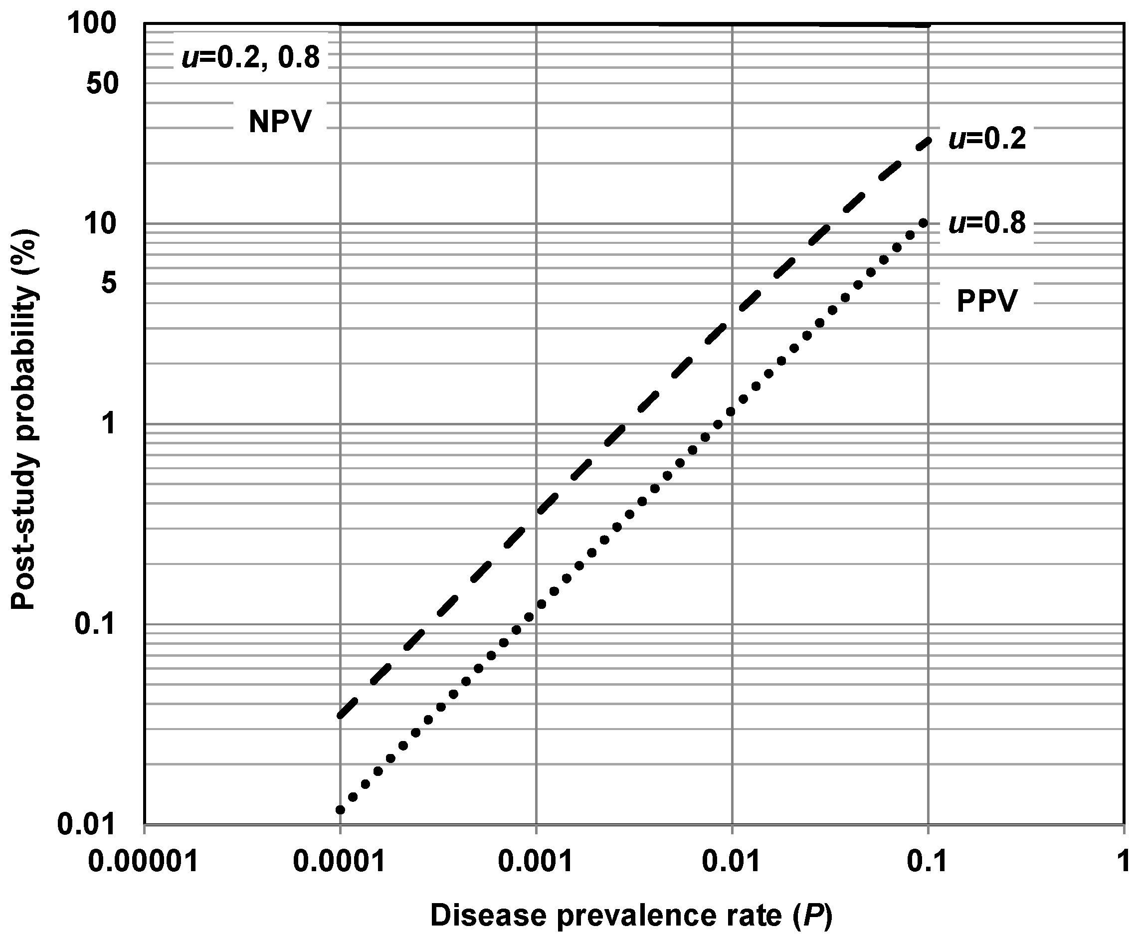
Table 1.
Estimates of prevalence for common chronic diseases of interest in United States.
| Disease Category | Disease | Population of Interest | Prevalence Rate (P) | Timeframe |
|---|---|---|---|---|
| Respiratory diseases | asthma | total males and females | 0.079 | in 2017 |
| chronic obstructive pulmonary disease (COPD) | adults ≥18 years | 0.059 | in 2014–2015 | |
| Heart diseases | coronary heart disease, angina or heart attack | adults ≥18 years | 0.056 | in 2018 |
| Diabetes | diabetes | total males and females | 0.094 | in 2015 |
| Cancers | breast | females ≥35 years | 0.037 | in 2016 |
| prostate | males ≥55 years | 0.072 | in 2016 | |
| colorectal | total males and females | 0.0040 | in 2016 | |
| lung and bronchus | total males and females | 0.0017 | in 2016 |
Note: Prevalence (P) is represented as a fraction (e.g., 0.0079 is 79 people out of 1000 for asthma). Refer to SI 1 for references upon which the prevalence rate (P) is based.
Table 2.
Three examples of search space analysis of a hypothetical observational study of ambient air quality versus hospitalization due to asthma exacerbation.
Table 2.
Three examples of search space analysis of a hypothetical observational study of ambient air quality versus hospitalization due to asthma exacerbation.
| Example 1 A simple univariate analysis of childhood asthma hospital admissions is considered using 6 air quality predictors—daily average levels of PM10, PM2.2, SO2, NO2, CO and O3, and no lags or weather covariate confounders: |
|
| Example 2 For a slightly more typical analysis of the same 6 predictors with 3 lags (i.e., same day, 1 and 2 day lags), and 2 weather variables treated as covariate confounders (daily average temperature and relative humidity), and also adjusting for possible confounding of co-pollutants in the analysis (i.e., air quality variables are also treated as covariate confounders in the analysis), we have the following search space counts: |
|
| Example 3 For a typical (and more in-depth) example, in addition to Example 2 characteristics, four different subgroups are used in the analysis (e.g., children ≤4 years, children 5–14 years, boys only ≤14 years and girls only ≤14 years) along with the main study population: |
|
* There are 7 covariates in Space 2—daily average temperature and relative humidity are 2 covariates; 1 pollutant is treated as a predictor adjusted with the other 5 pollutants (covariates) in the model.
Table 3.
Authors, variable counts, and analysis search spaces for the 17 randomly selected base papers from Zheng et al. [48].
Table 3.
Authors, variable counts, and analysis search spaces for the 17 randomly selected base papers from Zheng et al. [48].
| First Author | Outcomes | Predictors | Models | Lags | Covariates | Space1 | Space2 | Space3 |
|---|---|---|---|---|---|---|---|---|
| Thompson | 1 | 10 | 3 | 4 | 7 | 120 | 128 | 15,360 |
| Andersen | 3 | 11 | 1 | 6 | 8 | 198 | 256 | 50,688 |
| Chardon | 3 | 3 | 1 | 16 | 8 | 144 | 256 | 36,864 |
| Sheppard | 1 | 14 | 5 | 5 | 8 | 350 | 256 | 89,600 |
| Gouveia | 4 | 11 | 1 | 4 | 8 | 176 | 256 | 45,056 |
| Tenias | 1 | 24 | 4 | 4 | 5 | 384 | 32 | 12,288 |
| Magas | 4 | 6 | 1 | 2 | 5 | 48 | 32 | 1536 |
| Chakraborty | 1 | 3 | 2 | 1 | 4 | 6 | 16 | 96 |
| Tsai | 1 | 10 | 2 | 3 | 2 | 60 | 4 | 240 |
| Laurent | 4 | 4 | 3 | 6 | 5 | 288 | 32 | 9216 |
| Lavigne | 5 | 5 | 1 | 1 | 3 | 25 | 8 | 200 |
| Mar | 1 | 2 | 1 | 6 | 8 | 12 | 8 | 96 |
| Evans | 3 | 7 | 2 | 7 | 6 | 294 | 64 | 18,816 |
| Abe | 2 | 10 | 2 | 2 | 9 | 80 | 512 | 40,960 |
| Santus | 32 | 10 | 2 | 8 | 3 | 5120 | 8 | 40,960 |
| Hua | 2 | 2 | 8 | 5 | 4 | 160 | 16 | 2560 |
| Lin | 3 | 3 | 3 | 7 | 7 | 189 | 128 | 24,192 |
Note: Author name is first author listed (refer to SI 2); Space 1 = number of questions at issue = Outcomes × Predictors × Models × Lags; Space 2 = 2k where k = number of Covariates; Space 3 = approximation of analysis search space = Space 1 × Space 2.
Table 4.
Summary statistics for the number of possible tests using the three search spaces.
| Statistic | Space1 | Space2 | Space3 |
|---|---|---|---|
| minimum | 6 | 4 | 96 |
| lower quartile | 60 | 16 | 1536 |
| median | 160 | 32 | 15,360 |
| upper quartile | 288 | 256 | 40,960 |
| maximum | 5120 | 512 | 89,600 |
| mean | 450 | 118 | 22,866 |
Note: Space 1 = number of questions at issue = Outcomes × Predictors × Models × Lags; Space 2 = 2k where k = number of Covariates; Space 3 = approximation of analysis search space = Space 1 × Space 2.
Table 5.
Risk Ratio (RR), Lower Confidence Level (LCL) and Upper Confidence Level (UCL) values and corresponding p-values calculated for base papers used by Zheng et al. [48] in their PM2.5 meta-analysis.
Table 5.
Risk Ratio (RR), Lower Confidence Level (LCL) and Upper Confidence Level (UCL) values and corresponding p-values calculated for base papers used by Zheng et al. [48] in their PM2.5 meta-analysis.
| Study 1st Author 1 | Publication Year | RR | LCL | UCL | p-Value 2 |
|---|---|---|---|---|---|
| Lee SL | 2006 | 1.024 | 1.014 | 1.035 | 0.0001 |
| Ko FWS | 2007 | 1.004 | 1.000 | 1.009 | 0.0803567 |
| Jalaludin BB | 2008 | 1.017 | 1.008 | 1.027 | 0.000432 |
| Lavigne E | 2012 | 1.000 | 0.909 | 1.121 | 1 |
| Stieb DM | 2009 | 1.011 | 0.987 | 1.037 | 0.3923886 |
| Chimonas MAR | 2007 | 0.992 | 0.964 | 1.024 | 0.6144624 |
| Sluaghter JC (ER) | 2005 | 1.030 | 0.980 | 1.090 | 0.279572 |
| (H) | 1.010 | 0.910 | 1.110 | 0.8548709 | |
| Li S | 2011 | 1.032 | 1.007 | 1.057 | 0.010805 |
| Mar TF | 2010 | 1.000 | 0.957 | 1.043 | 1 |
| Sheppard L | 1999 | 1.034 | 1.017 | 1.059 | 0.001249 |
| Yamazaki S (W) | 2013 | 0.958 | 0.776 | 1.182 | 0.7025466 |
| (C) | 1.039 | 0.883 | 1.222 | 0.6573244 | |
| Santus P | 2012 | 0.991 | 0.970 | 1.011 | 0.399061 |
| Babin S | 2008 | 1.000 | 0.990 | 1.020 | 1 |
| Kim SY | 2012 | 1.009 | 0.991 | 1.026 | 0.3161553 |
| Paulu C | 2008 | 1.010 | 0.960 | 1.060 | 0.7070236 |
| Halonen JI (A) | 2008 | 1.003 | 0.957 | 1.050 | 0.907147 |
| (O) | 1.068 | 1.014 | 1.131 | 0.0180712 | |
| Szyszkowicz M | 2008 | 1.085 | 1.010 | 1.166 | 0.025766 |
| Malig BJ | 2013 | 1.020 | 1.010 | 1.030 | 0.0001 |
| Evans KA | 2013 | 0.821 | 0.418 | 1.403 | 0.5339787 |
| Ito K | 2007 | 1.060 | 1.052 | 1.072 | 0.0001 |
| Chardon B | 2007 | 1.044 | 0.999 | 1.104 | 0.0909348 |
| Lin M | 2002 | 1.011 | 0.925 | 1.065 | 0.7736097 |
| Silverman RA | 2010 | 1.075 | 1.050 | 1.100 | 0.0001 |
| Barnett AG (0–4y) | 2005 | 1.045 | 1.018 | 1.071 | 0.000713 |
| (5–14y) | 1.034 | 0.992 | 1.076 | 0.1067006 | |
| Iskandar A | 2012 | 1.188 | 1.083 | 1.271 | 0.0001 |
| Santus P | 2012 | 0.992 | 0.967 | 1.017 | 0.5433122 |
| Strickland MJ | 2010 | 1.022 | 1.002 | 1.042 | 0.029066 |
| Andersen ZJ | 2008 | 1.300 | 1.000 | 1.640 | 0.037304 |
| Hua J | 2014 | 1.003 | 1.000 | 1.010 | 0.2403955 |
| Gleason JA | 2014 | 1.012 | 1.000 | 1.024 | 0.048279 |
| Raun LH | 2014 | 1.033 | 0.983 | 1.083 | 0.1901706 |
| Cheng MH (W) | 2014 | 1.069 | 1.034 | 1.103 | 0.0001 |
| (C) | 1.017 | 1.000 | 1.046 | 0.1420481 |
1 letters/numbers in brackets indicates results for different population subgroups from the same study. 2 bold, italicized p-value < 0.05 calculated after [79].
Table 6.
Summary information about numbers of base papers and significant results used for meta-analysis for each air quality component.
Table 6.
Summary information about numbers of base papers and significant results used for meta-analysis for each air quality component.
| Air Quality Component | Number of Risk Ratios (RRs) Used | RRs with p-Values > 0.05 (%) | RR with p-Values ≤ 0.05 | RRs with p-Values ≤ 0.001 |
|---|---|---|---|---|
| CO | 42 | 29 (69) | 13 | 9 |
| NO2 | 66 | 30 (45) | 36 | 16 |
| O3 | 71 | 40 (56) | 31 | 11 |
| PM2.5 | 37 | 22 (59) | 15 | 8 |
| PM10 | 51 | 28 (55) | 23 | 6 |
| SO2 | 65 | 46 (70) | 19 | 6 |
Publisher’s Note: MDPI stays neutral with regard to jurisdictional claims in published maps and institutional affiliations. |
© 2021 by the authors. Licensee MDPI, Basel, Switzerland. This article is an open access article distributed under the terms and conditions of the Creative Commons Attribution (CC BY) license (https://creativecommons.org/licenses/by/4.0/).
Share and Cite
MDPI and ACS Style
Kindzierski, W.; Young, S.; Meyer, T.; Dunn, J. Evaluation of a Meta-Analysis of Ambient Air Quality as a Risk Factor for Asthma Exacerbation. J. Respir. 2021, 1, 173-196. https://0-doi-org.brum.beds.ac.uk/10.3390/jor1030017
AMA Style
Kindzierski W, Young S, Meyer T, Dunn J. Evaluation of a Meta-Analysis of Ambient Air Quality as a Risk Factor for Asthma Exacerbation. Journal of Respiration. 2021; 1(3):173-196. https://0-doi-org.brum.beds.ac.uk/10.3390/jor1030017
Chicago/Turabian StyleKindzierski, Warren, Stanley Young, Terry Meyer, and John Dunn. 2021. "Evaluation of a Meta-Analysis of Ambient Air Quality as a Risk Factor for Asthma Exacerbation" Journal of Respiration 1, no. 3: 173-196. https://0-doi-org.brum.beds.ac.uk/10.3390/jor1030017