Investigation of Environmentally Dependent Movement of Bottlenose Dolphins (Tursiops truncatus)

Abstract

How environmental features (e.g., people, enrichment, or other animals) affect movement is an important element for the study of animal behavior, biomechanics, and welfare. Here we present a stationary overhead camera-based persistent monitoring framework for the investigation of bottlenose dolphin (Tursiops truncatus) response to environmental stimuli. Mask R-CNN, a convolutional neural network architecture, was trained to automatically detect 3 object types in the environment: dolphins, people, and enrichment floats that were introduced to stimulate and engage the animals. Detected objects within each video frame were linked together to create track segments across frames. The animals’ tracks were used to parameterize their response to the presence of environmental stimuli. We collected and analyzed data from 24 sessions from bottlenose dolphins in a managed lagoon environment. The seasons had an average duration of 1 h and around half of them had enrichment (42%) while the rest (58%) did not. People were visible in the environment for 18.8% of the total time (∼4.5 h), more often when enrichment was present (∼3 h) than without (∼1.5 h). When neither enrichment nor people were present, the animals swam at an average speed of 1.2 m/s. When enrichment was added to the lagoon, average swimming speed decreased to 1.0 m/s and the animals spent more time moving at slow speeds around the enrichment. Animals’ engagement with the enrichment also decreased over time. These results indicate that the presence of enrichment and people in, or around, the environment attracts the animals, influencing habitat use and movement patterns as a result. This work demonstrates the ability of the proposed framework for the quantification and persistent monitoring of bottlenose dolphins’ movement, and will enable new studies to investigate individual and group animal locomotion and behavior.

1. Introduction

Features in an animal’s environment have the potential to influence behavior, biomechanics and movement patterns during daily life. For animals in managed settings, monitoring movement patterns to inform welfare practices is essential [1,2,3]. Behavior and movement patterns in response to common or long-term events in the surrounding environment can be predictable and identifiable [4,5,6]. For example, terrestrial animal studies [7] have shown that fixed feeding times during the day can result in stable and predictable behavior in stump-tailed macaques under human care. Previous animal studies have also investigated how enrichment and human interaction affect dolphin behavior in managed settings with trained observers monitoring and recording behavior [1,8]. Key to the identification of how these environmental conditions influence the animals is the ability to measure and quantify movement without influencing behavior [9]. Traditionally, trained researchers directly observe and manually record animal behavior, but this approach can be time consuming and is limited to when the animals are visible to the observer [1,8]. Observational approaches also tend to be qualitative, and are not capable of capturing the kinematics (position, speed, acceleration) of the animals as they move in the environment.

Biologging tags, which consist of sensors that record animal movement, sound, video, and other environmental measures, are used to provide high resolution measurements from animals [10,11]. Tags provide direct measurements of kinematics, but do not capture much information about the environmental context that may be driving behavior. Additionally, the animals have to be trained to wear the tags, and drag forces, high acceleration swimming or interactions with other animals can detach the sensors [12,13]. Camera data have been used in conjunction with direct observation to quantify swimming kinematics and body posture [10,14]. Camera systems installed in the environment enable continuous records of movement, environmental use, social interaction, and animal kinematics [13,14,15,16,17,18,19]. For shorter duration sessions, manual tracking is possible [20], however this becomes intractable as video lengths grow. Ideally, cameras could be used to persistently monitor animals and their environment for days or weeks at a time, but this requires robust automated object tracking methods with sufficient precision to characterize animal movement.

Here we implement an automated computer vision framework using methods from robotics to track bottlenose dolphins, people, and enrichment in a lagoon environment, and investigate how the presence of enrichment influences movement. Computer-automated animal tracking in a managed environment has only been explored recently, with initial research employing hand-crafted detection methods [6,16], later followed by a convolutional neural-network approach [17]. The method used in this work, Mask R-CNN [21], is a state-of-the-art object detection technique that is an enhancement of the Faster R-CNN detector [22] employed in [17]. Mask R-CNN was chosen for its additional precision over the older method, and the ability to extract object profiles. Using this algorithm to simultaneously mask and track the animals as they engage and respond to people and enrichment provides important kinematic information to quantify movement during these conditions.

For the experiment, video data were recorded at midday from animals in the main lagoon at Dolphin Quest (Oahu) during an extended period of unstructured swimming, both with and without enrichment. Positions and contours of dolphins, people and enrichment were extracted from the video frames and used to form dynamic tracks (tracklets). Animal kinematics (position, speed, heading) from these tracks were used to investigate how the animals move in the environment both with and without enrichment. These data were also used to score dynamic interactions between animals and enrichment, a first step towards quantification of animal preference for different enrichment types. Importantly, the computer-vision-based approach presented has broad applicability, and can be implemented to quantify movement and behavior as long as cameras can be installed in the environment, e.g., [16,17,18,19].

2. Materials and Methods

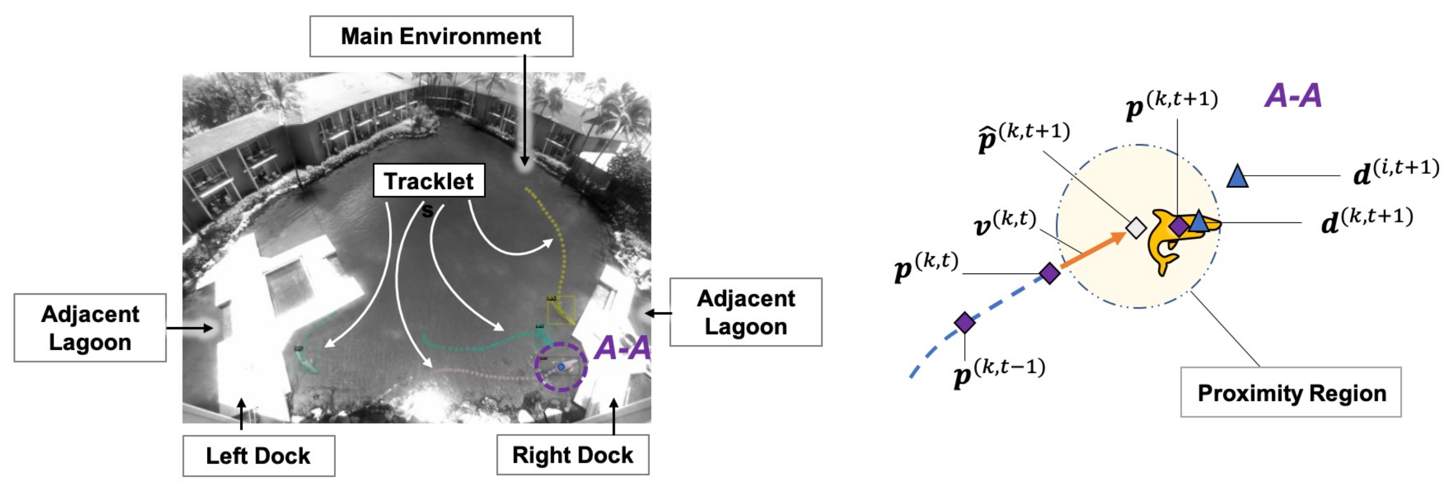
2.1. Environment Setups

The proposed research was conducted in the main lagoon environment at Dolphin Quest Oahu, Hawaii. The lagoon is ~36 m wide and ~54 m long, with two floating docks separating the main environment from two adjacent lagoons. The docks are used by the animal care specialists to move within the lagoon system and interact with the animals. During the trials, the movement of the animals in the lagoon was recorded using a stationary overhead camera (Allied Vision Manta G-319) with a wide angle lens (Kowa LM4NCL ½” 3.5 mm F/1.4 C-Mount Lock Screw Industrial Lens) equipped with a linear glass polarizing filter (Edmund Optics, 70 mm unmounted linear polarizer, wavelength range 400 to 700 nm) mounted using custom 3D-printed hardware. The wide angle lens (with polarizing filter) was calibrated using the Fisheye Camera Calibration tools in MATLAB and was able to capture the entire lagoon, along with the animal care specialists when present on the docks. Data from four bottlenose dolphins were collected over 24 days during periods of free swimming at midday, with hour long sessions taking place from 12:00 pm to 1:00 pm or from 1:00 pm to 2:00 pm. During these lunchtime sessions the animals moved freely in the environment, and the natural lighting conditions improved the ability to observe the dolphins when swimming underwater.

Animal care specialists were free to move within the environment during the trials. For half of the sessions one of two types of floating enrichment was introduced into the environment: red soft rounded jolly balls or black cylindrical buoys. Jolly Balls are smaller and dolphins can grasp them with their mouth when swimming, while Buoys are larger and harder for the dolphins to bring underwater. Both enrichment types have been routinely presented to the animals by the animal care specialists on a pseudo randomized schedule prior to this study as a means to promote welfare.

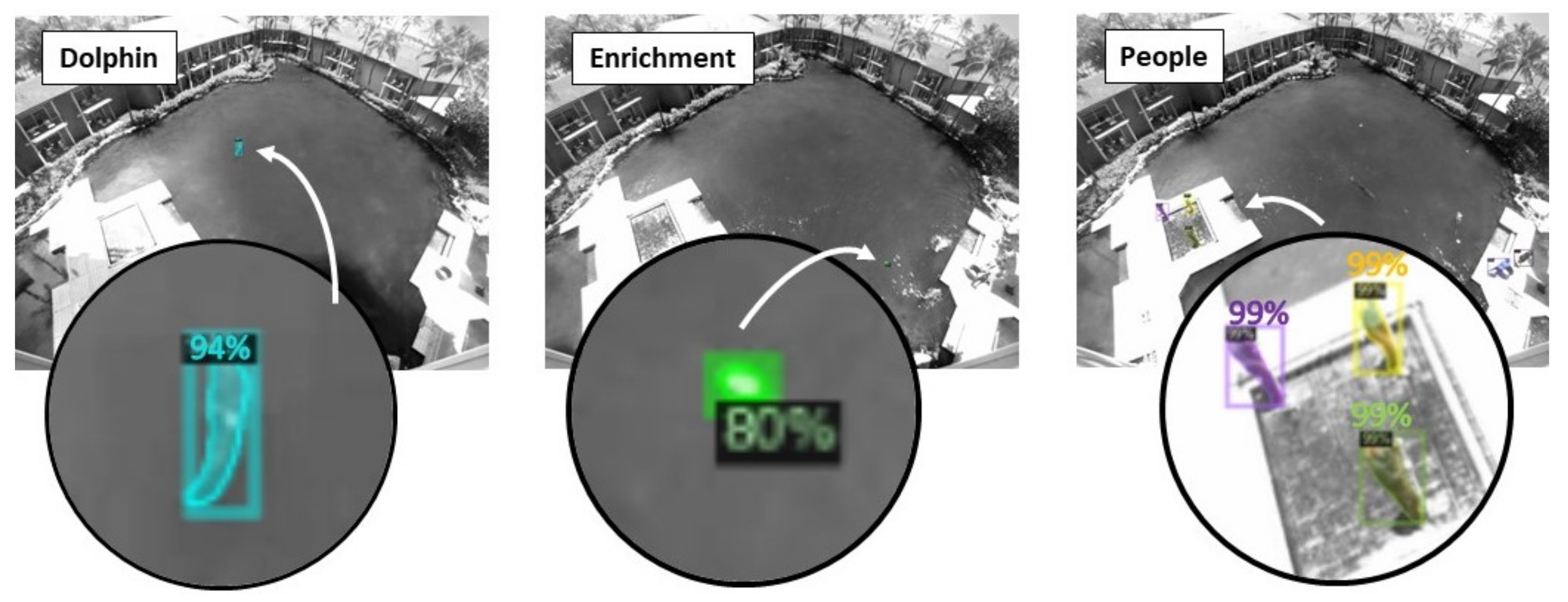
2.2. Target Detection

Three objects were detected and tracked in this study to explore how environmental stimuli affect animal movement: dolphins, people (animal care specialists) and floating enrichment. A convolutional neural network, Mask R-CNN [21], was implemented and trained to detect the object types from multi-hour video recordings. Mask R-CNN outputs include instance detection, classification and pixel-level object segmentation. Objects in the overhead video data are small and lack detail. Mask R-CNN was selected for this work because it is a well developed and validated object segmentation method, making it possible to reliably detect and mask objects using a more limited set of image features.

The model was trained using a dataset composed of 1200 frames selected from two 1-h sessions in August 2020. An additional 50 labeled frames for each type of enrichment were selected from 2 days to supplement the original training dataset. Objects (dolphins, people, enrichment) were manually annotated using the VGG Image Annotator [23], a stand-alone software package for manually annotating images. Each annotated object was also manually traced for the masking. Half of the labeled data were used to train the Mask R-CNN model, and the other half were used to test the classification results. The assessment results of the prediction confidence coefficient for the three detectors were greater than 80% (Figure 1). The camera frame rate was down sampled to 5 Hz, and the detectors were used to process 24 data sets collected in August, September, and October 2020.

The position of each detected object was estimated as the geometric center point of its mask and was transformed to correct for fisheye lens distortions using the Fisheye Camera Calibration tools in MATLAB. The corrected detections were mapped from the camera reference frame to the world reference frame by implementing a perspective transformation homography [24] and then used for the kinematic analysis.

2.3. Tracklet Formation and Kinematics

The world reference frame detections were initially independent for each image frame. To extract dynamic information from the targets, continuous tracklets were generated by applying a prediction-association constant velocity Kalman filter framework [16,24] to the detections across video frames, Figure 2. This prediction-association process forms a tracklet by identifying a detection in the next frame that could be associated with the current track. Based on the detection information in the current frame at time t, where ${\mathit{p}}^{(\mathit{k},\mathit{t})}=[{\mathit{p}}_{\mathit{x}}^{(\mathit{k},\mathit{t})},{\mathit{p}}_{\mathit{y}}^{(\mathit{k},\mathit{t})}]$ is the filtered position and ${\mathit{v}}^{(\mathit{k},\mathit{t})}=[{\mathit{v}}_{\mathit{x}}^{(\mathit{k},\mathit{t})},{\mathit{v}}_{\mathit{y}}^{(\mathit{k},\mathit{t})}]$ is the corresponding velocity of the k-th tracklet, the target’s predicted position (${\widehat{\mathit{p}}}^{(\mathit{k},\mathit{t}+1)}$) and velocity (${\widehat{\mathit{v}}}^{(\mathit{k},\mathit{t}+1)}$) in the next frame (t + 1) is obtained using a constant velocity model:

$$\begin{array}{cc}\hfill & {\mathit{v}}^{(\mathit{k},\mathit{t})}=({\mathit{p}}^{(\mathit{k},\mathit{t})}-{\mathit{p}}^{(\mathit{k},\mathit{t}-1)})/\Delta \mathit{t},\hfill \end{array}$$

(1)

$$\begin{array}{cc}\hfill & {\widehat{\mathit{p}}}^{(\mathit{k},\mathit{t}+1)}={\mathit{p}}^{(\mathit{k},\mathit{t})}+{\mathit{v}}^{(\mathit{k},\mathit{t})}\Delta \mathit{t},\hfill \end{array}$$

(2)

$$\begin{array}{cc}\hfill & {\widehat{\mathit{v}}}^{(\mathit{k},\mathit{t}+1)}={\mathit{v}}^{(\mathit{k},\mathit{t})}.\hfill \end{array}$$

(3)

If the position of the closest detection (${\mathit{d}}^{(\mathit{k},\mathit{t}+1)}$) in the next frame falls into the proximity region drawn from Kalman-predicted position ${\widehat{\mathit{p}}}^{(\mathit{k},\mathit{t}+1)}$, it is identified as an associated point for tracklet k at the time (t + 1) and used to generate the next filtered position ${\mathit{p}}^{(\mathit{k},\mathit{t}+1)}=\mathit{f}\mathit{i}\mathit{l}\mathit{t}\mathit{e}\mathit{r}({\widehat{\mathit{p}}}^{(\mathit{k},\mathit{t}+1)},{\mathit{d}}^{(\mathit{k},\mathit{t}+1)})$. If there are no detections within the proximity region at time step (t + 1), the predicted position (${\widehat{\mathit{p}}}^{(\mathit{k},\mathit{t}+1)}$) and velocity (${\widehat{\mathit{v}}}^{(\mathit{k},t+1)}$), are used to propagate the model forward, i.e., ${\mathit{p}}^{(\mathit{k},\mathit{t}+1)}={\widehat{\mathit{p}}}^{(\mathit{k},\mathit{t}+1)}$ and ${\mathit{v}}^{(\mathit{k},\mathit{t}+1)}={\widehat{\mathit{v}}}^{(\mathit{k},\mathit{t}+1)}$. If the number of unassociated frames grows larger than five time steps, the tracklet is considered inactive and is truncated at the last confirmed association. The speed ($\left|\mathit{v}\right|$) and heading (h) of an animal at time t correspond to the magnitude and direction of the filtered velocity vector ${\mathit{v}}^{(\mathit{k},\mathit{t})}$, respectively. Although heading rate ($\dot{\mathit{h}}$) is the derivative of heading:

$$\begin{array}{cc}\hfill & \left|\mathit{v}\right|=\sqrt{{\mathit{v}}_{\mathit{x}}^2+{\mathit{v}}_{\mathit{y}}^2},\hfill \end{array}$$

(4)

$$\begin{array}{cc}\hfill & \mathit{h}=arctan\frac{{\mathit{v}}_{\mathit{y}}}{{\mathit{v}}_{\mathit{x}}},\hfill \end{array}$$

(5)

$$\begin{array}{cc}\hfill & {\dot{\mathit{h}}}^{\left(\mathit{t}\right)}=({\mathit{h}}^{\left(\mathit{t}\right)}-{\mathit{h}}^{(\mathit{t}-1)})/\Delta \mathit{t}.\hfill \end{array}$$

(6)

2.4. Movement in the Environment

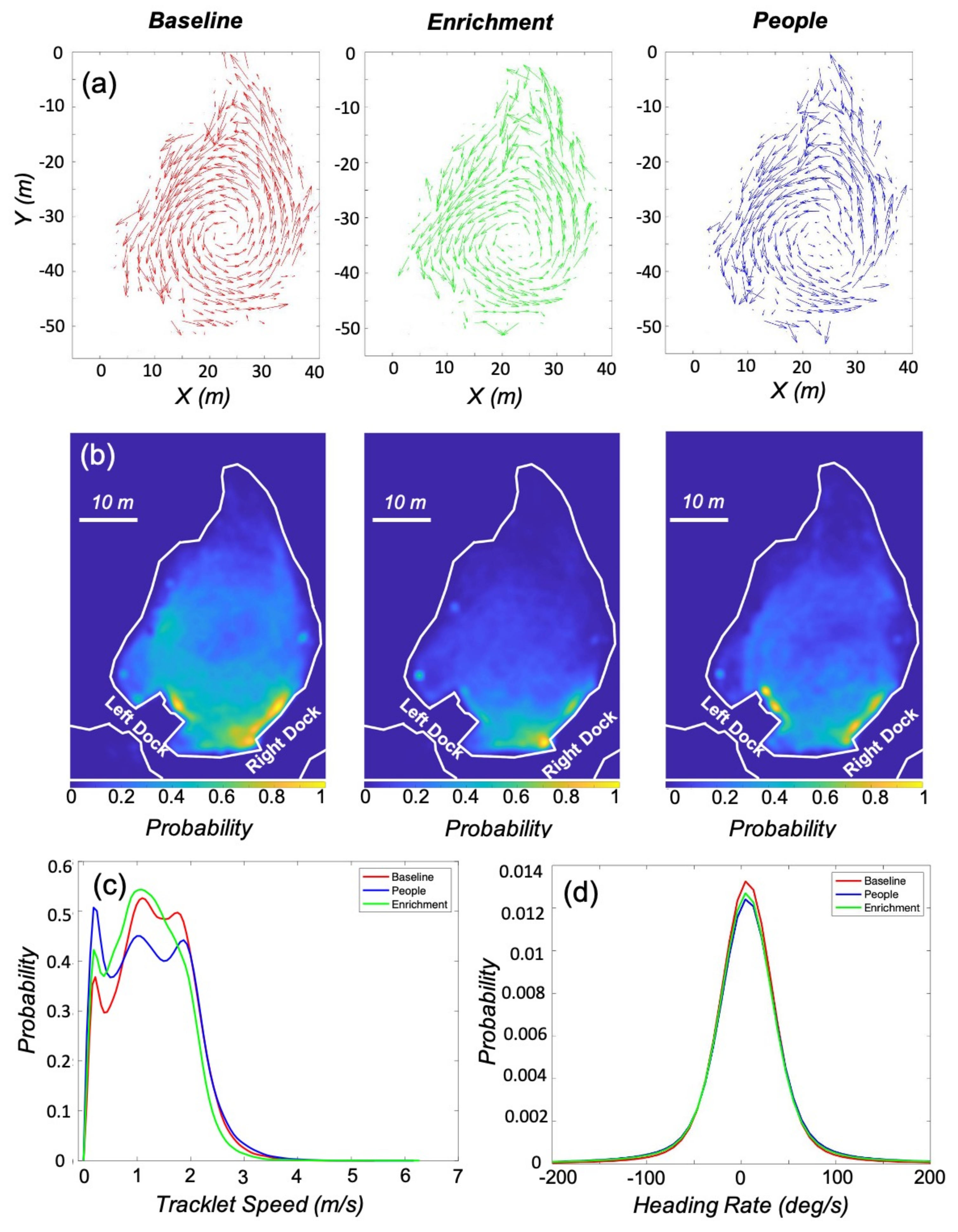
2.4.1. Occupancy Heatmaps and Flow in the Environment

Occupancy heatmaps were use to characterize where the animals tended to spend time during the experiment [5]. The heatmaps were generated by integrating the occupancy probability distribution for all detections onto a blank map. The maximum occupancy density was then scaled to 1 for each heatmap, resulting in a relative habitat use for each condition. Percentage Use of the habitat was then calculated as:

$$\mathrm{Percentage}\mathrm{Use}=\frac{{\mathit{A}}_{(0,1]}}{\mathit{A}},$$

(7)

where, A denotes the whole lagoon area and ${\mathit{A}}_{(0,1]}$ is the area where detections occurred (Probability greater than 0). Quiver plots were used to visualize the flow of the moving animals [24]. The environment was first subdivided into individual 2 m × 2 m cells. Vector headings for all tracklets that fell within an individual cell were then summed. If the animals tended to travel in the same direction as they passed through a cell, the summation adds and the resulting flow vector will have greater magnitude. Similarly, if the animals rarely move through a cell or if they move through a cell in many different directions, the resulting magnitude of the flow will be small.

2.4.2. Probability Density

Probability density functions for speed and heading rate were numerically determined for each experimental condition. A two-sample Kolmogorov-Smirnov (K-S) test [25] was used to compare the numerically derived distributions for movement in the presence of people and enrichment with the baseline condition. Comparing the density functions provides insight into trends present in the animals’ movements during different environmental conditions. The K-S test statistic returns the maximum absolute difference between the empirical cumulative distributions of the two compared datasets. Critical values were determined using a 0.05 significance level, and the numbers of data points used to generate the density functions were: 416,257 for the baseline condition, 213,631 for the enrichment, and 196,185 when people were present. If a K-S statistic is greater than its critical value, the null hypothesis, that the two datasets share the same distribution, is rejected.

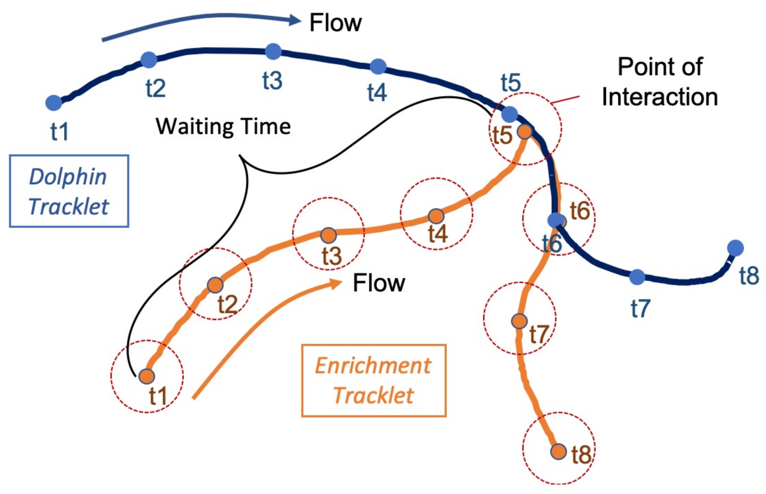
2.5. Engaging with Enrichment

A scoring system was used to evaluate how attractive enrichment introduced into the environment was for the dolphins. Data from four trails, two with buoys and two with jolly balls, were examined for this analysis. The number of observed interactions, and the time taken by the animals to engage with enrichment, waiting time, were used to parameterize enrichment attractiveness. Using this parameter we would expect animals to engage with an attractive piece of enrichment quickly and frequently, while a less attractive object will ‘wait’ longer for an interaction. Waiting time was calculated as the difference between the start time of an enrichment tracklet and the time when an animal tracklet passes within 2 m of the enrichment. The example in Figure 3 illustrates a single interaction where the waiting time is the difference between t1 and t5 for the orange enrichment tracklet. To summarize the data, the hour long sessions were partitioned into eighteen 200 s bins. Average waiting time was calculated for all animal–enrichment interactions within that bin. Only enrichment tracklets with recorded interactions were included in the average.

3. Results

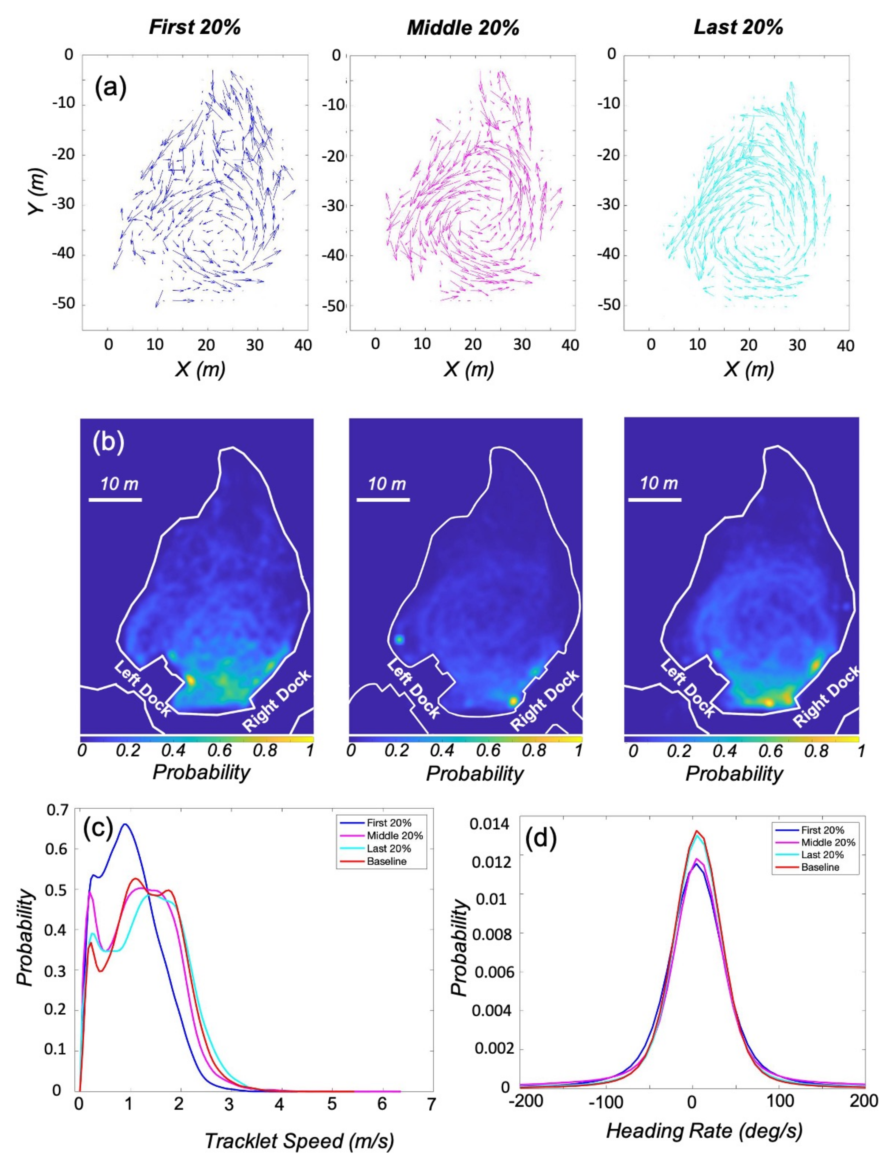
3.1. Kinematic Analysis

During the experiment, ∼9.5 h of baseline data and ∼10 h of data with enrichment were collected. Over the course of all the trials, people were present in the environment for ∼4.5 h, with ∼1.5 h of which involved no enrichment. The remaining ∼3 h of data had both enrichment and people present, and was excluded from the analysis. During this time, there were around 825,000 detections of the three objects in the environment. Figure 4a presents the flow of the animals, and indicates a general counter-clockwise movement during all three conditions. The pattern of movement does vary between conditions, with a less defined center of rotation when enrichment or people were present. During the experiment the animals had a preference for areas in the environment near the docks for all three conditions, Figure 4b. The normalized probability was highest, the yellow areas, near both docks during the baseline and people conditions, and near the right dock when enrichment was present. During the baseline condition, the animals had a larger and more defined circular area of use in the center of the environment, indicating more time spent in the circular counter-clockwise motion present in the flow. The percentage use of the environment was also the largest for the baseline condition, with an 89.3%, 72.6%, and 79.7% use for the baseline, enrichment, and people, respectively.

The probability density functions calculated for speed and heading rate are presented in Figure 4c,d. All three conditions had mean heading rates of 5 deg/s, confirming the counter-clockwise motion observed in the flow. Mean speed during the baseline condition (1.2 m/s) was higher than when either enrichment or people were present in the environment. The peaks in the density functions at the lower speeds (>0.5 m/s) indicate periods with little forward motion. This first peak is highest when people were present and lowest during the baseline condition. The density for baseline speed was used for comparison with the other two conditions (people and enrichment) in the two-sample Kolmogorov-Smirnov test. The resulting difference between the cumulative distribution of the baseline condition and the enrichment condition was 0.07, while the difference with people present was 0.08. The differences with the baseline distribution were small for both conditions, but both test statistics are greater than the corresponding critical values (

Table 1. Summary measures calculated from the tracklets for the three conditions (baseline, enrichment, and people). Mean, standard deviation, and the results of the K-S tests are reported. The enrichment and people conditions are compared with Baseline in the K-S tests.

Parameter (Condition)	Mean	Standard Deviation	K-S Test Statistic	Critical Values
Speed (Baseline)	1.20 m/s	0.74	0	0
Speed (Enrichment)	1.01 m/s	0.73	0.07	0.0036
Speed (People)	1.09 m/s	0.81	0.08	0.0037
Heading Rate (Baseline)	5.63 deg/s	43.01	0	0
Heading Rate (Enrichment)	5.33 deg/s	54.65	0.03	0.0036
Heading Rate (People)	5.94 deg/s	55.18	0.04	0.0037

).

3.2. Enrichment

The first 20%, middle 20%, and final 20% of the enrichment trials were examined to investigate how movement patterns change over time with enrichment present in the environment. The ∼2 h of data for each period were used to generate quiver plots and heatmaps, Figure 5. The motion of the animals was more variable when enrichment was first introduced, with a more defined counter-clockwise movement pattern returning by the last 20 % of the trials. The heatmaps indicate that the animals were more likely to be present in the bottom half of the lagoon between the docks during the first 20%, with hotspots near the right dock as the trials progressed. By the last 20% of the trials the circulate motion of the animals was again visible in the heatmap. The percentage use of the environment for the three periods were 75.33%, 61.79%, 67.06%. The mean speed of the animals increased from 1 m/s to 1.33 m/s over the course of the trials. The mean heading rate was around 5 deg/s for all three periods,

Table 2. Report the statistic of the tracklets’ speed and heading rate for the first 20%, middle 20%, and last 20% time sessions under enrichment condition. All three sessions were compared with the Baseline condition in the K-S tests.

Parameter (Condition)	Mean	Standard Deviation	K-S Test Statistic	Critical Values
Speed (First 20%)	1.00 m/s	0.57	0.21	0.0064
Speed (Middle 20%)	1.20 m/s	0.69	0.06	0.0058
Speed (Last 20%)	1.33 m/s	0.72	0.03	0.0062
Heading Rate (First 20%)	4.26 deg/s	54.89	0.07	0.0064
Heading Rate (Middle 20%)	5.56 deg/s	74.04	0.05	0.0058
Heading Rate (Last 20%)	5.95 deg/s	52.77	0.01	0.0062

.

The density functions for the three periods are compared to the baseline distribution in Figure 5c,d. The probability distribution for the speed during the first 20% of the enrichment trials is visibly different from the other three, with slower overall speeds and a higher probability of slow forward motion (>0.5 m/s). The density for baseline speed was again used for comparison with the other two conditions in the two-sample Kolmogorov-Smirnov test. The K-S tests indicate that as the enrichment trials progressed, the probability distributions for speed and heading rate both became more similar to the baseline distributions, Table 2. All K-S test statistics for speed exceeded the critical values, but the difference between the cumulative distribution of the baseline condition and the first 20% was the largest at 0.21, and decreased to 0.03 for the last 20% of the trials. The K-S test statistics for the heading rate were all small and ranged from 0.07 to 0.01, but all exceeded their corresponding critical values.

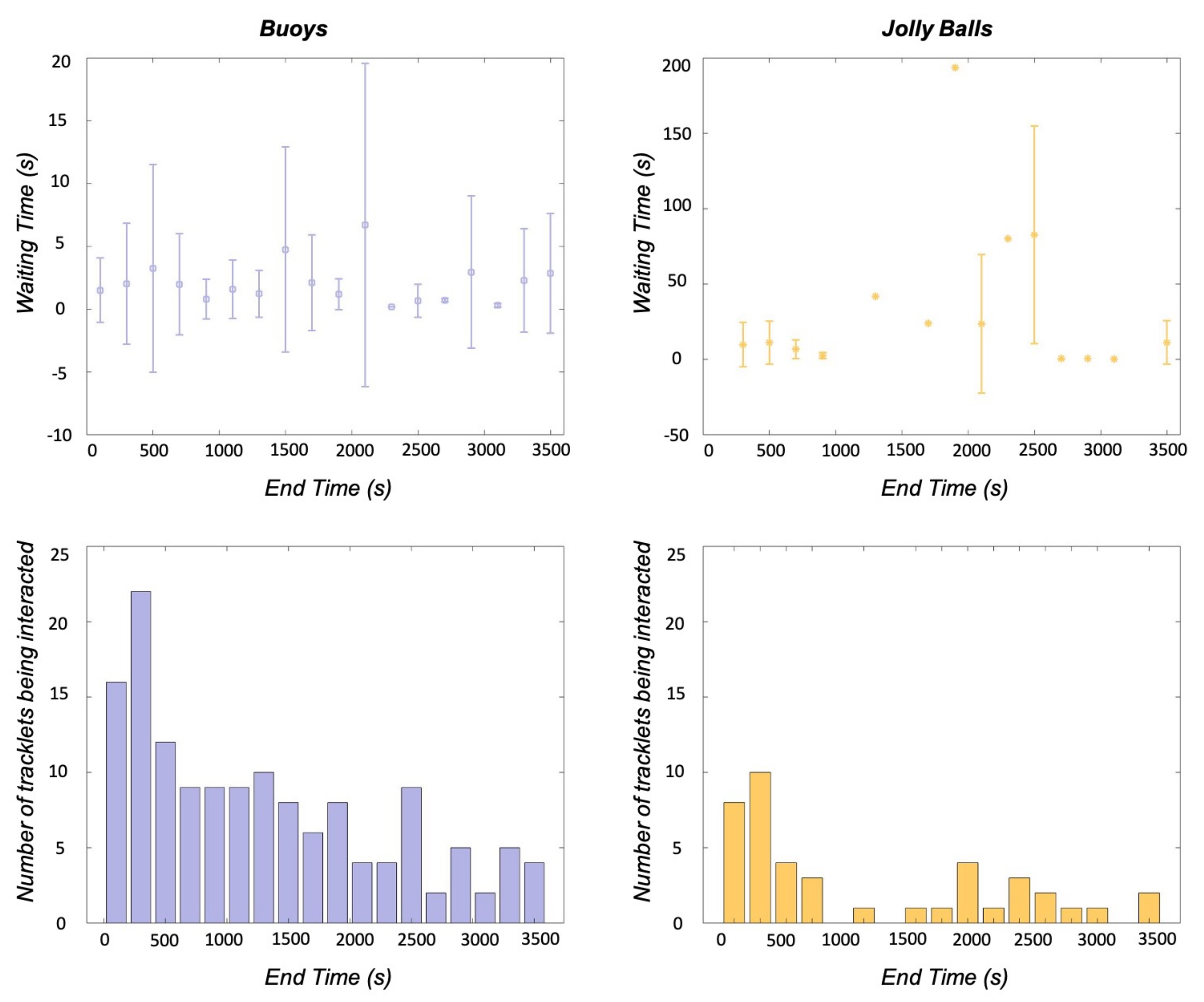
3.3. Enrichment Engagement

Waiting time was used to further investigate interactions between the animals and enrichment. A 4-trial subset of the data, two hours with buoys and two hours with jolly balls, was used to evaluated engagement with the enrichment. Figure 6 presents waiting time and interaction counts for both types of enrichment. The average waiting time for the buoys was 2.0 s (4.7 SD), with the average waiting time per bin never exceeding 10 s. However, the number of interactions decreased throughout the trial, beginning with interaction counts as high as 20, but ending with counts between 1 and 5 for the 200-second-wide bins. The waiting time for the jolly balls had a higher average, 22.1 s (41.7 SD), and was more variable, with times ranging from 0.2 to 193.6 s. The number of interactions with the jolly balls was lower than the buoys (144 vs. 42), but the same decreasing trend is present in the data.

4. Discussion

The ability to monitor how animals move in their environment while also identifying contextual factors that may influence movement is a challenging problem. In this work, we presented a computer vision based persistent monitoring and analysis framework to quantify bottlenose dolphin movement. Direct monitoring by trained behaviorists and observers provides important information about the animals in their environments. These observations are qualitative, and can be supplemented with information from cameras and other sensors placed in or around the environment. As sensing becomes integrated into more environments, the ability to efficiently and effectively extract information from sensor data will be key to maximizing the benefits of these systems. In this work, more than 21 h of data were examined, resulting in over 850,000 detected objects for the analysis. This detection density enabled the extraction of important animal kinematics (speed, heading, heading rate) that were used to characterize motion. If a trained observer were able to manually score one detection every second, it would take more than nine days of continuous work to label the entire dataset presented here. Further, the trained network can be used to classify objects from additional datasets, creating the opportunity to investigate behavior over the course of months or even different seasons.

To demonstrate the approach, we analyzed video data from four animals observed during hour long unstructured swimming trials in a lagoon environment at midday. Enrichment was present for half the sessions, and animal care specialists were free to move in the environment during the recordings. Qualitative differences from baseline are visible in the directional quiver plots and occupational heatmaps when enrichment or people were present. A general counter-clockwise flow was observed in the animal movement during all environmental conditions (i.e., baseline, enrichment, and people), Figure 4. This flow pattern is consistent with the previous observations that dolphins tend to swim in a counter-clockwise direction in the Northern Hemisphere when staying in a defined environment [26]. Although clockwise preferential swimming biases have been observed for dolphins in the Southern Hemisphere, it is speculated that the dominating flow direction is the result of global forces rather than individual dolphin anatomy [27].

Proximity to the docks occurred more frequently in the baseline condition than when enrichment was present. During baseline, the animals were observed swimming, interacting with another animal (e.g., paired swimming), or inspecting the adjacent lagoons separated by the floating docks. In the heatmaps, there were no people present on the docks, but the increased time spent near these areas could be driven by multiple reasons. It could be the result of their inspection of animals in neighboring lagoons, their interaction with the structure of the dock, an association of the docks with the trainers, or an anticipatory behavior. When enrichment was present the average speed decreased from 1.2 m/s (baseline) to 1.0 m/s, and the animals spent more time in the bottom half of the lagoon. Overall area of use also decreased from 89.3% to 72.6%. These changes in spacial distribution could be due to enrichment distribution in the lagoon. Enrichment was introduced from the docks, and wind would push the floating enrichment to the edges of the lagoon biasing distribution and the resulting animal movement.

The K-S statistics indicate that the speed and heading rate probability distributions when enrichment or people were present are different from the baseline condition, Table 1. Speed distributions have two sets of peaks: a first peak between 0 and 0.5 m/s and a second set of peaks between 0.5 and 4 m/s, Figure 4c. The first peak indicates a distinct period of time when the animals were swimming slowly or were stationary. The highest first peak probability occurred when people were present in the environment. A higher probability might be expected because this condition includes periods of time at the start and end of the trials when the animals were at station with the animal care specialists. Additional peaks in the probability functions around 1 m/s and 2 m/s are present during the baseline condition and when people are present. The distribution for the enrichment condition has a single peak around 1 m/s, which is in accordance with the overall drop in speed when enrichment is present. The probability distributions for the heading rate all indicate that the animals are turning counter-clockwise, confirming the direction of the flow in the quiver plots, Figure 4d.

Engagement with the enrichment was further investigated by calculating how often the animals interacted with the enrichment floats and how this changed over the course of the trial, Figure 5 and Figure 6. When enrichment was introduced, the first 20% of the trial, there is less circularity in the movement flow and the animals tended to remain between the two docks in the bottom part of the lagoon. The K-S test statistic for speed distribution during the first 20% of the enrichment condition (0.21) shows the largest difference with baseline movement of and condition, Table 1 and Table 2. However, as the trial progressed distributions for speed and heading rate reverted towards baseline behavior with K-S differences of 0.3 and 0.1, respectively. These temporal changes were also seen in the analysis of enrichment engagement.

Interactions between the animals and two types of enrichment floats (Buoys and Jolly Balls) were examined to demonstrate how this approach can be used to quantify animal movement and environmental features simultaneously. Engagement with the enrichment was quantified using interaction counts, and time duration between an interaction and the initial detection (waiting time). For the buoys, the average waiting time (2 s vs. 22 s) was shorter than for the Jolly Balls and the total number of interactions (144 vs. 42) was higher. The interaction counts for the first 20% of the trials (0–720 s) were the highest for both enrichment types, Buoys = ∼56 and Jolly Balls = ∼21, and dropped off considerably for the last 20% of the trials (2880–3600 s), Buoys = ∼11 and Jolly Balls = ∼4. These temporal changes could again be due to the distribution of the enrichment in the environment as wind tended to gradually blow the enrichment to the edges of the lagoon. Because the animals spend more time in the center of the lagoon environment, reducing the likelihood of encountering enrichment at the edge of the environment. Additionally, accessing the enrichment at the shallow rocky edges of the lagoon could be more difficult for the animal further reducing the opportunity for engagement. On the other hand, the animals ‘letting’ the enrichment be slowly blowing to the edges of the lagoon could also indicate habituation to the specific enrichment. The two types of floating enrichment were physically similar when compared to other enrichment categories (e.g., food dispensing enrichment, trainer involved enrichment, etc. [28,29,30,31]), yet the animals could still prefer one over the other. Jolly Balls are small and round with light colors that can be carried by mouth when swimming, while Buoys are larger and more difficult to bring underwater. The animals’ variable response to the two types of floating enrichment could result from the different interaction mechanisms or simply the physical appearance of the objects. It is of great interest to extend this work to investigate and compare animals’ response to other types of enrichment (e.g., food dispensing enrichment, trainer involved enrichment, etc. [28,29,30,31]) as a means to detect improvements in welfare.

The results of the computer vision based monitoring and analysis framework are promising, but there are limitations to consider. If different types of enrichment are introduced, new detectors will have to be trained using labeled data. Additionally, the detectors for this work were trained on data collected from the same time of day. To use these detectors with images from other periods of time, it may be necessary to retrain the network with images that cover a wide range of lighting conditions with the objects of interest. A single overhead camera mounted towards the bottom of the lagoon was used to collect the data for this work. A second camera placed to better observe the top half of the lagoon would improve the coverage of the environment. Biologging tags could also be used in conjunction with the monitoring cameras to achieve continuous monitoring of the animal [16,17] at the cost of the introduction of biologging tags.

5. Conclusions

A computer vision based persistent monitoring and analysis framework was presented to efficiently and effectively extract dolphin kinematics, and track the movement of people and enrichment in the environment. This ability to simultaneously extract animal kinematics and the factors that may influence movement is an important complement to direct monitoring by trained behaviorists and observers. The framework was used to investigate bottlenose dolphin movement during three conditions: baseline, with enrichment and with people. Animal kinematics (position, speed, heading, heading rate) were automatically extracted from over 21 h of video footage, at a resolution that would be infeasible to label manually. A general counter-clockwise swimming flow was observed during the three conditions, and the presence of both enrichment and people in the environment did modify the observed kinematics. These changes were largest when enrichment was first introduced, with animal movement largely returning to baseline by the final 20% of the trials. The proposed framework is flexible and can be implemented in other facilities where overhead video data can be collected, enabling new data streams for the investigation of animal movement in these environments.

References

1. Kagan, R.; Carter, S.; Allard, S. A Universal Animal Welfare Framework for Zoos. J. Appl. Anim. Welf. Sci. 2015, 18 (Suppl. 1), S1–S10. [Google Scholar] [CrossRef] [PubMed] [Green Version]
2. Whitham, J.C.; Wielebnowski, N. New Directions for Zoo Animal Welfare Science. Appl. Anim. Behav. Sci. 2013, 147, 247–260. [Google Scholar] [CrossRef]
3. Miller, L.J.; Vicino, G.A.; Sheftel, J.; Lauderdale, L.K. Behavioral Diversity as a Potential Indicator of Positive Animal Welfare. Animals 2020, 10, 1211. [Google Scholar] [CrossRef] [PubMed]
4. Daan, S. Adaptive Daily Strategies in Behavior. In Biological Rhythms; Springer: Boston, MA, USA, 1981; pp. 275–298. [Google Scholar]
5. Stamps, J.A. Individual Differences in Behavioural Plasticities: Behavioural Plasticities. Biol. Rev. Camb. Philos. Soc. 2016, 191, 534–567. [Google Scholar] [CrossRef]
6. Karnowski, J.; Hutchins, E.; Johnson, C. Dolphin Detection and Tracking. In Proceedings of the 2015 IEEE Winter Applications and Computer Vision Workshops, Waikoloa, HI, USA, 5–9 January 2015. [Google Scholar]
7. Waitt, C.; Buchanan-Smith, H.M. What Time Is Feeding? Appl. Anim. Behav. Sci. 2001, 75, 75–85. [Google Scholar] [CrossRef]
8. Mason, G.J. Species Differences in Responses to Captivity: Stress, Welfare and the Comparative Method. Trends Ecol. Evol. 2010, 25, 713–721. [Google Scholar] [CrossRef] [PubMed] [Green Version]
9. Mcbride, A.F.; Hebb, D.O. Behavior of the Captive Bottle-Nose Dolphin, Tursiops Truncatus. J. Comp. Physiol. Psychol. 1948, 41, 111–123. [Google Scholar] [CrossRef]
10. Johnson, M.P.; Tyack, P.L. A Digital Acoustic Recording Tag for Measuring the Response of Wild Marine Mammals to Sound. IEEE J. Ocean. Eng. 2003, 28, 3–12. [Google Scholar] [CrossRef] [Green Version]
11. Zhang, D.; Shorter, K.A.; Rocho-Levine, J.; van der Hoop, J.; Moore, M.; Barton, K. Behavior Inference from Bio-Logging Sensors: A Systematic Approach for Feature Generation, Selection and State Classification. In Proceedings of the ASME 2018 Dynamic Systems and Control Conference, Atlanta, GA, USA, 30 September–3 October 2018; Volume 2. [Google Scholar]
12. Van der Hoop, J.M.; Fahlman, A.; Hurst, T.; Rocho-Levine, J.; Shorter, K.A.; Petrov, V.; Moore, M.J. Bottlenose Dolphins Modify Behavior to Reduce Metabolic Effect of Tag Attachment. J. Exp. Biol. 2014, 217 Pt 23, 4229–4236. [Google Scholar] [CrossRef] [Green Version]
13. Zhang, D.; Hoop, J.M.; Petrov, V.; Rocho-Levine, J.; Moore, M.J.; Shorter, K.A. Simulated and Experimental Estimates of Hydrodynamic Drag from Bio-logging Tags. Mar. Mamm. Sci. 2020, 36, 136–157. [Google Scholar] [CrossRef]
14. Sibal, R.; Zhang, D.; Rocho-Levine, J.; Shorter, K.A.; Barton, K. Bidirectional LSTM Recurrent Neural Network plus Hidden Markov Model for Wearable Sensor-Based Dynamic State Estimation. ASME Lett. Dyn. Syst. Control 2021, 1, 1–6. [Google Scholar] [CrossRef]
15. Fish, F.E.; Legac, P.; Williams, T.M.; Wei, T. Measurement of Hydrodynamic Force Generation by Swimming Dolphins Using Bubble DPIV. J. Exp. Biol. 2014, 217 Pt 2, 252–260. [Google Scholar] [CrossRef] [Green Version]
16. Gabaldon, J.; Zhang, D.; Barton, K.; Johnson-Roberson, M.; Shorter, K.A. A Framework for Enhanced Localization of Marine Mammals Using Auto-Detected Video and Wearable Sensor Data Fusion. In Proceedings of the 2017 IEEE/RSJ International Conference on Intelligent Robots and Systems (IROS), Vancouver, BC, Canada, 24–28 September 2017. [Google Scholar]
17. Zhang, D.; Gabaldon, J.; Lauderdale, L.; Johnson-Roberson, M.; Miller, L.J.; Barton, K.; Shorter, K.A. Localization and Tracking of Uncontrollable Underwater Agents: Particle Filter Based Fusion of on-Body IMUs and Stationary Cameras. In Proceedings of the 2019 International Conference on Robotics and Automation (ICRA), Montreal, QC, Canada, 20–24 May 2019. [Google Scholar]
18. Tanaka, H.; Li, G.; Uchida, Y.; Nakamura, M.; Ikeda, T.; Liu, H. Measurement of Time-Varying Kinematics of a Dolphin in Burst Accelerating Swimming. PLoS ONE 2019, 14, e0210860. [Google Scholar] [CrossRef]
19. Rachinas-Lopes, P.; Ribeiro, R.; Dos Santos, M.E.; Costa, R.M. D-Track-A Semi-Automatic 3D Video-Tracking Technique to Analyse Movements and Routines of Aquatic Animals with Application to Captive Dolphins. PLoS ONE 2018, 13, e0201614. [Google Scholar] [CrossRef] [PubMed]
20. van der Hoop, J.M.; Fahlman, A.; Shorter, K.A.; Gabaldon, J.; Rocho-Levine, J.; Petrov, V.; Moore, M.J. Swimming Energy Economy in Bottlenose Dolphins under Variable Drag Loading. Front. Mar. Sci. 2018, 5. [Google Scholar] [CrossRef]
21. He, K.; Gkioxari, G.; Dollar, P.; Girshick, R. Mask R-CNN. In Proceedings of the IEEE International Conference on Computer Vision, Venice, Italy, 22–29 October 2017. [Google Scholar]
22. Ren, S.; He, K.; Girshick, R.; Sun, J. Faster R-CNN: Towards Real-Time Object Detection with Region Proposal Networks. arXiv 2015, arXiv:1506.01497. [Google Scholar] [CrossRef] [Green Version]
23. Dutta, A.; Zisserman, A. The VIA Annotation Software for Images, Audio and Video. In Proceedings of the 27th ACM International Conference on Multimedia, Nice, France, 21–25 October 2015; ACM: New York, NY, USA, 2019. [Google Scholar]
24. Gabaldon, J.; Zhang, D.; Lauderdale, L.; Miller, L.; Johnson-Roberson, M.; Barton, K.; Shorter, K.A. Vision-based monitoring and measurement of bottlenose dolphins’ daily habitat use and kinematics. bioRxiv 2021. Forthcoming. [Google Scholar]
25. Berger, V.W.; Zhou, Y. Kolmogorov—Smirnov test: Overview. In Wiley StatsRef: Statistics Reference Online; John Wiley & Sons, Ltd.: Hoboken, NJ, USA, 2014. [Google Scholar]
26. Sobel, N.; Supin, A.Y.; Myslobodsky, M.S. Rotational Swimming Tendencies in the Dolphin (Tursiops Truncatus). Behav. Brain Res. 1994, 65, 41–45. [Google Scholar] [CrossRef]
27. Stafne, G.M.; Manger, P.R. Predominance of Clockwise Swimming during Rest in Southern Hemisphere Dolphins. Physiol. Behav. 2004, 82, 919–926. [Google Scholar] [CrossRef]
28. Kuczaj, S.; Lacinak, T.; Fad, O.; Trone, M.; Solangi, M.; Ramos, J. Keeping environmental enrichment enriching. Int. J. Comp. Psychol. 2002, 15, 127–137. [Google Scholar]
29. Harley, H.E.; Fellner, W.; Stamper, M.A. Cognitive research with dolphins (Tursiops truncatus) at Disney’s The Seas: A program for enrichment, science education, and conservation. Int. J. Comp. Psychol. 2010, 23, 331–343. [Google Scholar]
30. Lauderdale, L.K.; Miller, L.J. Common Bottlenose Dolphin (Tursiops Truncatus) Problem Solving Strategies in Response to a Novel Interactive Apparatus. Behav. Process. 2019, 169, 103990. [Google Scholar] [CrossRef] [PubMed]
31. Lauderdale, L.K.; Miller, L.J. Efficacy of an Interactive Apparatus as Environmental Enrichment for Common Bottlenose Dolphins (Tursiops truncatus). Anim. Welf. 2020, 29, 379–386. [Google Scholar] [CrossRef]
Figure 1. Example detections of a dolphin, floating enrichment (a buoy), and people in the lagoon environment. Each detected object is shown with its corresponding mask and the likelihood of detection.
Jzbg 02 00023 g001
Figure 2. (Left) Detections and tracklets are shown for four animals in the lagoon. (Right) An illustration of the tracklet prediction-association-filtering process. Where for tracklet k the current filtered position is p ( k , t ) , the current filtered velocity is v ( k , t ) , the Kalman-predicted future position is p ^ ( k , t + 1 ) and the detection selected for filtering is d ( k , t + 1 ) , while the filtered position of the animal at the next step is p ( k , t + 1 ) . d ( i , t + 1 ) is another detection at (t + 1) that is not associated with the k-th tracklet.
Jzbg 02 00023 g002
Figure 3. An illustration of how waiting time was defined for the enrichment. Eight time steps are shown for a dolphin (blue) and a piece of enrichment (orange). A point of interaction occurs at t5 when the dolphin detection is within 2 m of the enrichment at the same time. The waiting time is then defined as the time from the initial detection (t1) to the point of interaction (t5).
Jzbg 02 00023 g003
Figure 4. Results comparing the three environmental conditions: baseline, enrichment, and people. (a) Quiver plots for all three conditions show counter-clockwise movement in the lagoon, with the most concentric pattern occurring during the baseline condition. (b) Position heatmaps for the conditions show how the presence of enrichment or people modified where the animals spent time in the environment. (c,d) Probability density functions for the speed and heading rate of the animals derived from the tracklets. The animals tended to swim faster during the baseline condition, and spent more time stationary when people where present in the environment. Mean heading rates for all three conditions were positive, indicating counter-clockwise swimming trend.
Jzbg 02 00023 g004
Figure 5. Animal movement when enrichment was present in the environment. (a) The quiver plots show a more varied movement pattern when enrichment is initially introduced. (b) The heatmaps also indicate that the use of the environment during the first 20% of the time with enrichment was more variable. For all three heatmaps, 1 in color bar represents the maximum occupancy density based on the corresponding conditions. (c,d) Probability density of tracklet speed and heading rate show that the animals tended to move faster during the middle and last 20%, and preference for counter-clockwise swimming was not as strong when the enrichment was initially introduced.
Jzbg 02 00023 g005
Figure 6. Average waiting time and standard deviation (top) and number of enrichment interactions (bottom) are shown for each 200-second-wide bins for two types of enrichment (Buoys and Jolly Balls). The waiting time for buoys is lower than that for Jolly Balls in general (note that the y-axes for waiting time are on different scales). The numbers of interactions for both enrichment show decreasing trends as the trials progress.
Jzbg 02 00023 g006