1. Introduction
Common bottlenose dolphins (hereafter referred to as ‘dolphins’),
Tursiops truncatus, that inhabit brackish inshore estuaries have been observed in salinities ranging from 15 to 25 ppt. These inshore dolphins can suffer adverse health effects from prolonged freshwater exposure and pollution introduced from surface runoff [
1,
2,
3,
4,
5], which can occur as a result of natural climatic events. For example, a high-precipitation event that coincided with local agricultural pesticide applications and reduced bay salinities to <10 ppt for several months was likely associated with a dolphin Unusual Mortality Event (UME), a period in which there is a significant die-off of a marine mammal population, along the mid-Texas coast [
6]. Poor water quality, prolonged freshwater exposure, and changes in water temperature were associated with increases in dolphin skin lesion prevalence and extent in multiple populations [
1,
2,
4,
7,
8]. Additionally, abrupt changes in water quality and salinity caused by floods were associated with the development of poxvirus-like skin lesions on Indo-Pacific bottlenose dolphins,
Tursiops aduncus [
9]. While an increasing number of studies show associations between poor water quality conditions, low salinities, and negative health complications in dolphins, there is still much to learn about how dolphins behaviorally respond to potentially harmful water quality conditions and low salinities in their habitat.
Natural climatic events, such as floods, can drastically alter water quality by affecting salinity, water temperature, dissolved oxygen (hereafter abbreviated as ‘DO’), pH, turbidity, nutrient levels, organic matter loadings, and primary productivity in estuaries over a short time period [
10,
11,
12], which can have impacts on dolphins. It may take several months for estuaries to return to normal levels, depending on the intensity of the flood [
10,
12]. Dolphins may respond to flood events by leaving the area and/or moving to areas with higher salinities. For example, Fury and Harrison [
10] found that Indo-Pacific bottlenose dolphins left two Australian estuary systems during flood events. Dolphins were more commonly found in higher-salinity areas, such as deep channels, following a hurricane that caused salinity to drop below 11 ppt for several weeks in Galveston Bay, Texas [
8]. Conversely, other studies have found that dolphins do not leave an area when water quality conditions deteriorate. Mazzoil and colleagues [
13] did not find correlations between dolphin density and salinity, sea surface temperature, and contaminant loads despite high levels of freshwater intrusion and contaminants from agricultural runoff in the Indian River Lagoon, Florida. In the Texas UME, stranding records showed that dolphins likely died inshore, suggesting that dolphins remained in the bay system despite low salinity levels and high concentrations of pesticides [
6]. Given the varied responses of dolphins to potentially harmful water quality conditions and low salinities, more information is needed to understand when and why dolphins choose to leave (or not leave) an area when water quality conditions deteriorate and whether dolphins are able to mitigate negative impacts from environmental changes. A record-breaking flood event in Pensacola Bay, Florida provided a natural experiment to explore how dolphins responded to abrupt changes in their environment.
On 29 April 2014, over 50 cm of rain fell in the Pensacola, Florida area [
14], resulting in an unprecedented three-meter freshwater surface layer over the entire Pensacola Bay estuary, which lasted several months [
15]. A population dynamics study on the inshore Pensacola Bay dolphin community was ongoing at the time [
15], providing an opportunity to examine dolphins’ behavioral response to this record-breaking flood. Twenty-seven percent of dolphins observed within three weeks of the flood had skin lesions, which was an increase in skin lesion prevalence compared to the previous session. Skin lesion prevalence remained elevated during flood conditions [
15]. However, only 20% of all identified dolphins observed within six months following the flood were seen with skin lesions [
16]. Additionally, there was no significant increase in mortality events following the flood based on local stranding data [
16]. Combined results indicate a lack of community-wide health complications [
16] despite unprecedented levels of sustained fresh water (<5 ppt) throughout the estuary and the influx of nutrients and contaminants from runoff (Table 2,
Figures S3–S8). Finally, there was no evidence of a decline in seasonal abundance following the flood to indicate that dolphins may have left the area [
15]. These results were surprising given the strength of the flood and the duration of flood-impact on the estuary. Pensacola Bay regularly experiences seasonal hypoxia and stratification of water temperature and salinity depending on the degree of mixing in the water column [
17]. Considering the regular occurrence of water column stratification and the large amount of freshwater intrusion during the flood, dolphins may have altered their distribution toward higher salinities in order to mitigate their freshwater exposure. The purpose here is to explore this hypothesis by examining noticeable dolphin distribution changes in response to the flood and determining whether dolphins avoided freshwater areas by moving south toward the estuary mouth and/or moving toward deeper water (>3 m) to get under the freshwater surface layer. Associations between environmental variables and dolphin distribution were also examined to identify environmental variables that potentially influence dolphin distribution during flood conditions. If dolphins avoided freshwater areas, it was expected that salinity and depth would be associated with dolphin distribution during flood conditions.
2. Materials and Methods
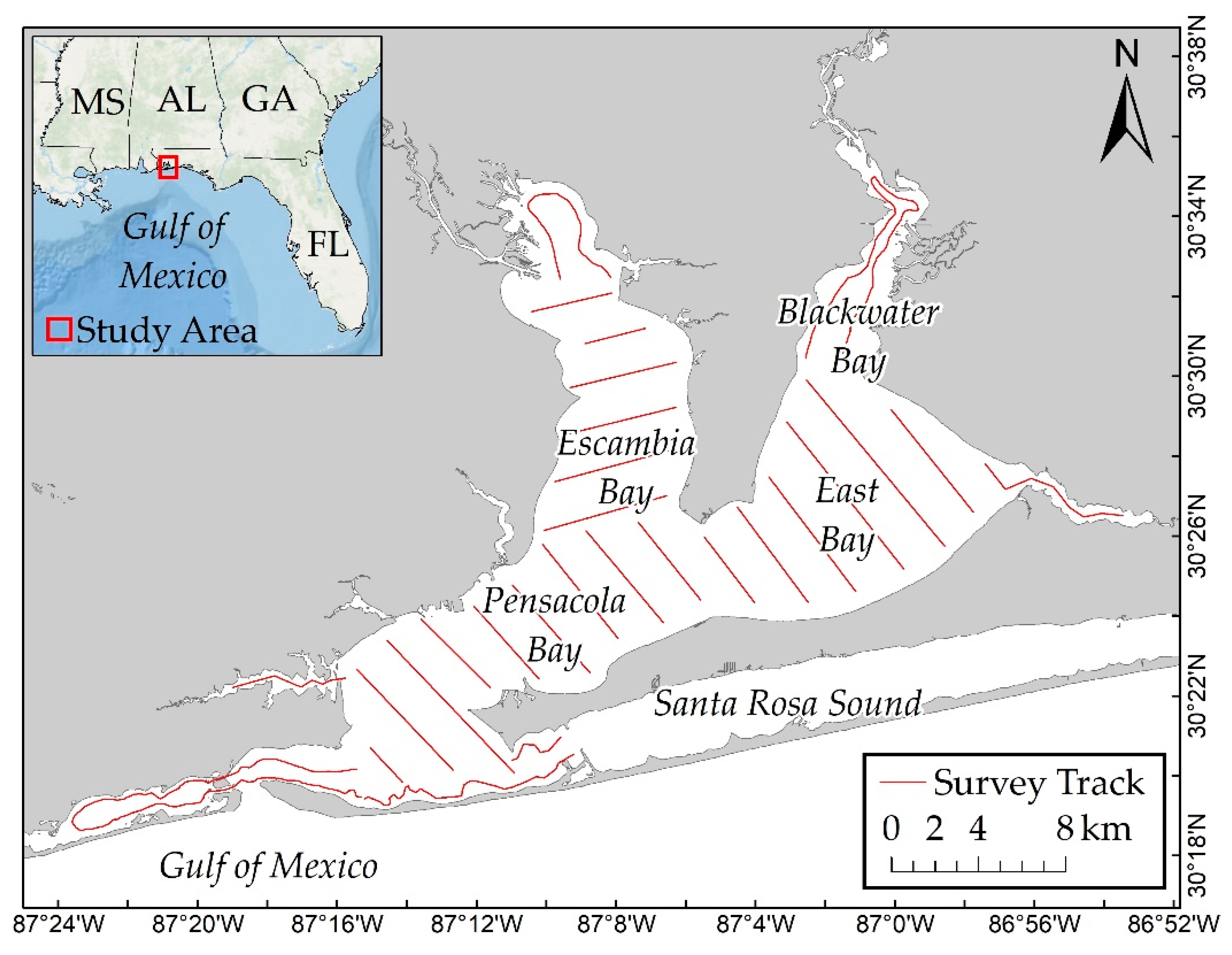
The Pensacola Bay system is located on the western Florida Panhandle and it consists of four interconnected estuaries: Blackwater, East, Escambia, and Pensacola Bays (
Figure 1).
This system has a vast watershed (~18,130 km
2) from Blackwater, Escambia and Yellow Rivers, which all drain into the bay [
18]. Pensacola Bay is connected to the Gulf of Mexico by a single narrow (~800 m wide) pass [
17]. The estimated average depth of the estuary system is 2.88 m (SD = 2.35 m) and ranges from approximately 0.15 to 10.5 m [
19]. Submerged aquatic vegetation (hereafter abbreviated as ‘SAV’) is located primarily in the southern region near the estuary mouth [
20].
Dolphin survey data from a boat-based population dynamics study [
15] were utilized for this study. Mark–recapture photo-identification surveys were conducted over a 2.5-year period (Summer 2013–Winter 2016), resulting in nine sampling sessions. Surveys were conducted in Beaufort Sea State ≤3. Dolphins were considered as part of the same group if they were within 100 m of each other and if they were generally moving in the same direction and engaging in the same activity [
21,
22]. The following information was recorded during dolphin sightings: GPS location, time, weather and sighting conditions, estimated group size and composition (i.e., adults, calves, and neonates), group activity, and environmental data, including surface salinity, water temperature, and DO that were recorded at the beginning of each dolphin sighting using a ©YSI instrument (Model 85).
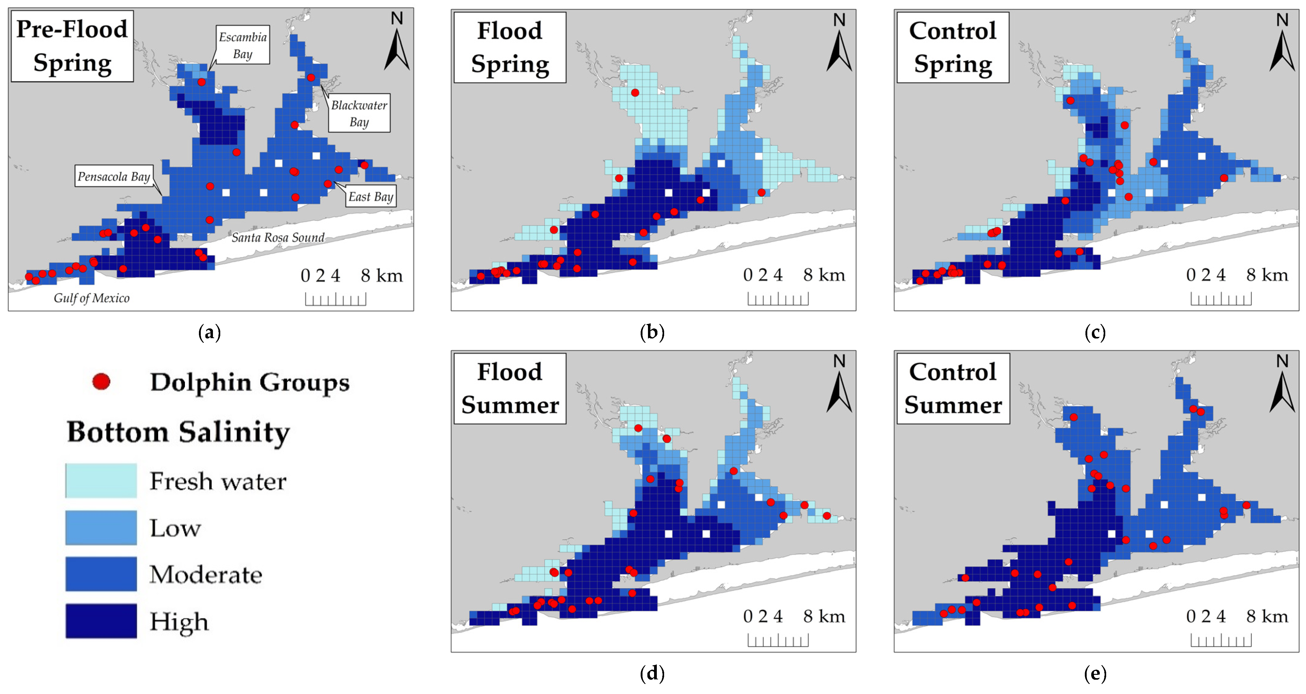
Dolphin survey data were organized into flood-impacted sessions and their respective seasonal control sessions unaffected by the flood event. Spring and Summer 2014 sessions were considered flood-impacted sessions (hereafter referred to as ‘Flood Spring’ and ‘Flood Summer’) based on the time it took for the freshwater surface layer to mix with salinities >11 ppt [
16,
17]. Consequently, Spring 2015 (hereafter referred to as ‘Control Spring’) served as the spring control session and it occurred one year after the flood. Summer 2013 (hereafter referred to as ‘Control Summer’) served as the summer control session and it occurred nine months before the flood. A sampling session was completed in March 2014, two months before the flood. This sampling session (hereafter referred to as ‘Pre-Flood Spring’) was retained for kernel density estimates to provide a baseline for early spring dolphin distribution prior to the flood.
Multiple sources in addition to dolphin surveys were used to acquire environmental data in order to maximize spatial coverage of the Pensacola Bay system. The Water Quality Portal (WQP), an online, public-access database of water quality data collected by multiple federal, state, and private organizations, was used to acquire samples of DO, salinity, water temperature, Kjeldahl nitrogen, and phosphorus [
23]. These data were queried to match the geographic survey area and time of dolphin surveys with an additional 2 weeks before and after surveys to increase sample size and spatial coverage. For Flood Spring, data were queried after the flood. Additionally, the local Environmental Protection Agency office monitors water quality conditions using CTD stations from northern Escambia Bay to the estuary mouth [
17]. CTD station samples were queried to match the temporal extent of queried WQP data. CTD station samples were not available for Control Summer and CTD stations did not collect nitrogen and phosphorus samples.
Due to seasonal hypoxia and water column stratification within Pensacola Bay [
17], samples for both surface and bottom salinity, water temperature, and DO were important to understand how dolphins may respond to water quality changes. Surface samples were collected at ≤0.25 m deep, which included recordings from dolphin surveys. Bottom samples were collected at the maximum depth from each available sampling station. Variables with sample data were interpolated using the Spline with Barriers tool in ArcGIS 10.X [
24] for each session.
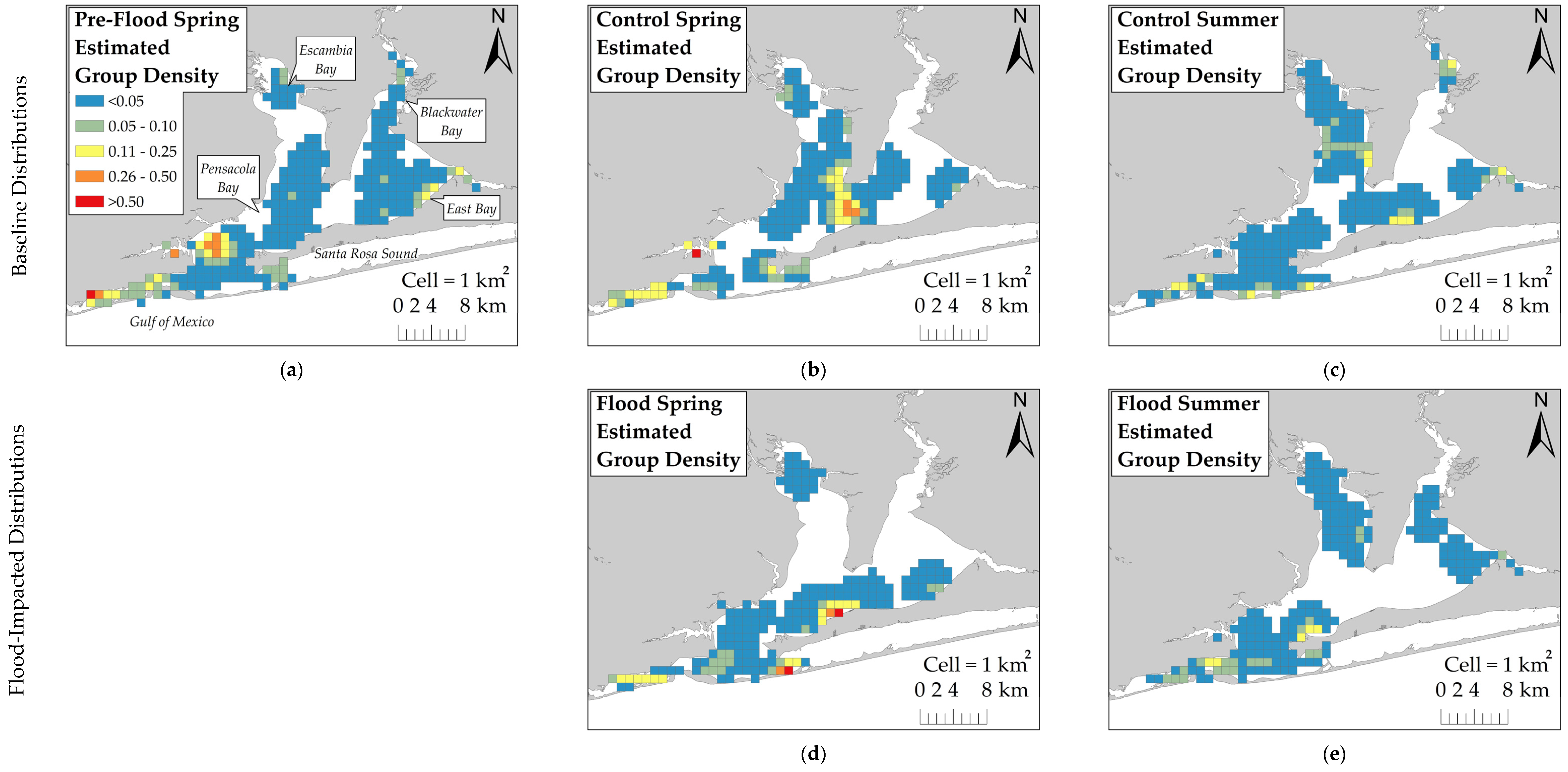
Analyses were completed in ArcGIS using a projected NAD 1983 16N spatial reference system. Dolphin group density (group/km) was summarized in a 1 km × 1 km grid over the survey area. The grid cell size was based on the average distance dolphins moved during observation (mean = 798 m; SD = 626 m). The number of dolphin groups was summarized for each cell in the grid using the start location coordinate of a group observation. The total number of on-effort survey kilometers (i.e., segments in which observers searched for dolphins) was summed in each cell for each session. The number of dolphin groups was divided by the number of survey kilometers to control for unequal survey effort across sessions.
The KDE with Barriers tool in ArcGIS was used to estimate group density across the survey area and control for land barriers that dolphins could not access. The href bandwidth [
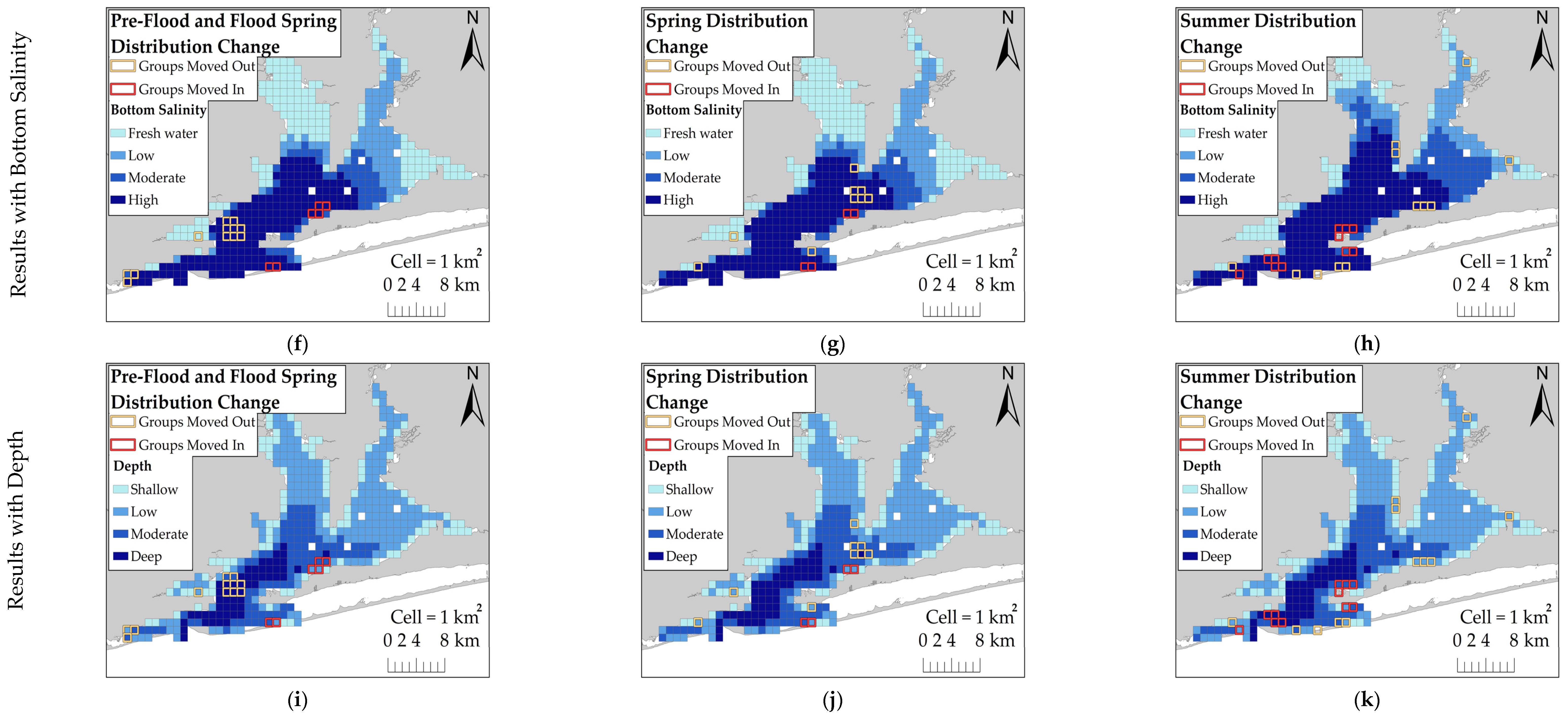
25] served as the KDE’s search radius. To compare fine-scale changes in estimated dolphin group density across sessions, the output KDE rasters were subtracted from each other using the Raster Calculator tool. Difference values that were greater than two standard deviations from the average estimated group density difference were considered significant changes in dolphin distribution.
The following environmental variables were summarized within each cell for each session: depth [
19], slope, slope standard deviation, distance from land [
26], distance from SAV [
20], latitude, longitude, surface and bottom salinity, surface and bottom water temperature, surface and bottom DO, Kjeldahl nitrogen, and phosphorus. These variables have been associated with dolphin distribution in other populations [
27,
28,
29,
30,
31,
32,
33,
34,
35]. Distance from land and SAV were calculated using the Near tool. Latitude and longitude were the decimal degree coordinates of the cell center. All remaining variables were summarized by performing spatial joins between their respective shapefiles and the grid containing dolphin group density for each session.
Regression-based species distribution models (SDMs) were used to determine associations between environmental variables and dolphin distribution in order to identify environmental variables that potentially influence distribution during flood conditions. Dolphin group density was the dependent variable and the environmental variables were predictor variables:
All variables were continuous variables except for flood period and season. Flood period was a categorical variable with two levels (Flood vs. Control) that were assigned to four sessions. The Pre-Flood Spring session was excluded from SDM analyses because it did not have a corresponding flood-impacted session. Season was a categorical variable with two levels: spring and summer. A Mann–Whitney U test was used to determine whether environmental variables differed across flood periods. Collinearity was examined across variables and highly correlated variables (r > 0.80) were removed from models [
36]. Main effects and interactions between environmental variables were tested using three model types. A generalized linear model (GLM) was used to explore parametric relationships between environmental variables and dolphin group density, which was a constrained response variable (>0 group/km) with a non-normal error distribution [
37]. A generalized additive model (GAM) was used to examine nonparametric relationships between these variables [
38]. A zero-altered gamma (ZAG) model was also tested because group density contained a high number (approximately 94%) of zeros which can impact dispersion for GLMs and GAMs. The ZAG model is a type of hurdle model that examines whether certain variables influence the presence–absence of dolphins by fitting a GLM to presence–absence data, and it examines whether certain variables influence dolphin group density by fitting a GLM to presence-only data [
39]. Once the best fit models for presence–absence data and presence-only data are determined, these models are combined into one model [
39]. All variables and their interactions were evaluated through backward stepwise comparisons in order to remove insignificant variables and avoid overfitting the model. The model with the lowest AIC was selected as the best fit model for each model type [
39]. The adjusted r
2 was used to determine how well the model explained variation in dolphin distribution. The model with the highest adjusted r
2 was selected as the overall best fit model. The predicted dolphin distribution derived from the best fit model was compared to the observed distribution in order to assess model performance. Modeling and post hoc analyses were performed in R [
37],
Supplemental Material 2.
4. Discussion
This study examined the behavioral response of dolphins to a record-breaking flood event in Pensacola Bay by comparing their distribution across flood-impacted sessions and control sessions. Dolphins did not exhibit a substantial change in distribution during flood-impacted sessions, but there was evidence of a small-scale change in distribution toward the south. KDE comparisons showed that dolphins moved south by one to several kilometers during flood-impacted sessions compared to control sessions. However, the ZAG model did not detect an association between dolphin distribution and latitude across flood periods. This finding suggests that the change in dolphin distribution towards the south by several kilometers was a limited population-wide distribution change. It is possible that detecting an extensive distribution change in Control Spring may not be feasible because dolphins were not regularly observed using the northern regions, such as Blackwater and East Bays, during the spring season. This infrequent use of the northern regions during the spring may be attributed to the seasonal distribution of prey. Many dolphin prey species migrate between inshore estuaries during warm months and coastal spawning areas during cold months [
41,
42]. In the spring, prey species are likely more heavily distributed in the southern regions as they migrate into the estuary. As water temperatures increase during the summer, prey species likely move further inshore. This potential inshore movement of prey may explain why dolphins moved into Escambia and East Bays during both Control Summer and Flood Summer. Dolphins were distributed throughout the estuary during both Control Summer and Flood Summer, but dolphins were more heavily concentrated further south and closer to the estuary mouth during Flood Summer compared to Control Summer. However, this summer distribution change towards the south was limited to several kilometers. The limited distribution change towards the south during flood-impacted sessions may have reduced the severity of flood effects, but dolphins were exposed to flood-induced water quality changes for several months.
This study also examined associations between environmental variables and dolphin distribution in order to identify environmental variables that may influence dolphin distribution during flood conditions. There was no evidence to support the hypothesis that dolphins moved to deeper areas with higher salinities during flood-impacted sessions. Dolphin group density was higher in shallow areas across all sessions which indicates dolphins did not move to deeper areas after the flood. It is possible that the use of shallow waters by Pensacola Bay dolphins is linked to their foraging activity. Dolphins have been observed to use shallow areas more often and to forage more often in shallow areas [
31,
32,
33,
35]. In Pensacola Bay, the river mouths offer an abundance of riverine fish species [
43], which could have offered a food source for dolphins at a time when marine prey species were negatively impacted by the flood.
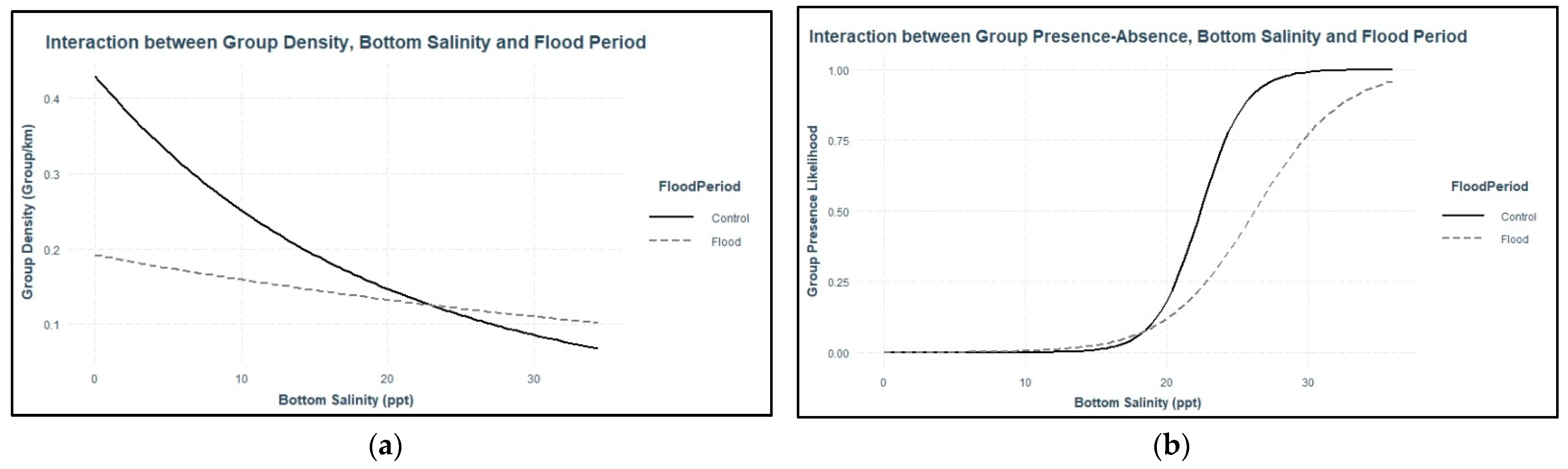
Dolphins were expected to use areas with higher salinity during flood-impacted sessions, but the association between dolphin distribution and salinity was not straightforward. During flood-impacted sessions, the majority of dolphin groups was observed in surface salinities ≤8 ppt and bottom salinities >20 ppt. There was no association between dolphin distribution and surface salinity across flood periods which suggests the three-meter freshwater surface layer throughout the estuary did not influence dolphin distribution. Considering that Pensacola Bay is prone to water column stratification [
17], dolphins may be habituated to low surface salinities. Bottom salinities appear to have some influence on dolphin distribution. Some dolphin groups used areas with lower bottom salinities, but the majority of dolphin groups used areas with higher bottom salinities across both flood-impacted sessions and control sessions. The relationship between bottom salinity and dolphin distribution was stronger during control sessions which suggests that the flood altered the bottom salinity thresholds for dolphin distribution. Low bottom salinities had a weaker effect on dolphin group density and higher bottom salinities were needed to increase the likelihood of dolphin presence during flood-impacted sessions compared to control sessions. Additionally, dolphin group density was higher during flood-impacted sessions compared to control sessions, but more groups were observed during control sessions. These results may be explained by dolphins exploiting a limited number of stratified areas with higher bottom salinities during flood-impacted sessions in order to avoid entirely freshwater areas. It is likely that dolphins regularly exhibit this behavioral response due to Pensacola Bay’s susceptibility to water column stratification during years of normal freshwater flow [
17], but the severity of this flood elicited a more pronounced behavioral response. Collectively, these data indicate that the majority of dolphins used stratified areas with higher bottom salinities and dolphin distribution was not substantially altered by the flood-induced salinity changes. This finding is unexpected given the magnitude and duration of flood impacts throughout the estuary. Pensacola Bay dolphins were anticipated to avoid low-salinity areas based on observations in Barataria Bay, Louisiana, where there was a low prevalence of dolphin telemetry locations in fresh water (<5 ppt) and a high prevalence in salinities ≥8 ppt [
44]. However, most of these dolphins were tagged near the barrier islands at the southern portion of the bay, where salinities stay fairly high. Recent tracking data from high site fidelity dolphins tagged further north in Barataria Bay demonstrated that some dolphins use low-salinity areas for weeks to months at a time, despite the availability of higher-salinity waters nearby. These dolphins exhibited variation in their use of low salinities across individuals to the extent that salinity was not significantly associated with their ranging patterns [
45]. Findings from both this study and recent evidence in Barataria Bay suggest that some dolphins regularly use low-salinity areas despite the potential health complications from prolonged low-salinity exposure. Alternatively, some dolphins may implement strategies to mitigate their low-salinity exposure through poorly understood mechanisms, either physiologically or through vertical habitat use not addressed in this study. For example, Pensacola Bay dolphins used stratified areas with broad salinity ranges instead of moving toward less stratified areas with higher salinities. Altering their vertical use of the water column may be a strategy for dolphins to reduce their low-salinity exposure while they continue to use potentially preferred habitat affected by the flood. This mitigation strategy is highly plausible considering the dolphins’ lack of avoidance toward low surface salinities and their frequent use of stratified areas with higher bottom salinities. Future research should consider examining whether dolphins change their swimming patterns in response to flood events (i.e., longer and/or deeper dive durations to spend more time in higher bottom salinities compared to surface fresh water).
The dolphins’ limited behavioral response to the flood may be partially explained by flood impacts on estuarine primary productivity and ecosystem dynamics. Dolphin distribution was associated with flood-induced changes in surface and bottom temperatures and higher concentrations of nitrogen and phosphorus. It is possible that changes in estimated nitrogen and phosphorus concentrations may not be accurately represented throughout the estuary due to limited sample coverage; however, increases in nitrogen and phosphorus concentrations after flood events have been observed in Pensacola Bay [
11]. Changes in temperature and nutrient loadings can affect estuarine primary productivity and ecosystem dynamics [
12,
46]. For example, overall fish numbers and fish species richness were low during flood events in Apalachicola Bay, Florida. However, fish biomass and species richness increased during the period following flood events which was likely attributed by changes in river flow, increased primary productivity, and trophic interactions among fish species [
46]. It is probable that prey availability within Pensacola Bay decreased during and immediately after the flood given the severity of the flood. This potential reduction in prey may explain why dolphins were more heavily distributed further south closer to the estuary mouth in Flood Spring compared to Control Spring because this location would allow dolphins to better exploit prey entering the estuary from coastal waters. However, the increase in nutrient concentrations following the flood is expected to stimulate primary productivity [
11], which influences fish abundance and species richness [
46]. Dolphins most likely moved to areas where primary productivity increased during the months after the flood in order to exploit prey that were attracted to these areas. Movement towards areas of higher primary productivity, and presumably increased prey availability, may explain why dolphins were distributed throughout the estuary during Flood Summer despite low salinities.
Additionally, the limited behavioral response of dolphins to the flood may be partially attributed to flood-induced changes in seasonal hypoxia, which may affect habitat suitability for many estuarine species. Low bottom DO had a stronger effect on dolphin distribution during control sessions compared to flood-impacted sessions. High freshwater inflow was observed to confine hypoxia to a smaller area in Pensacola Bay through displacement of strongly stratified water further south [
17]. This trend was observed for estimated bottom DO values in Control Summer and Flood Summer and average bottom DO was higher during flood-impacted sessions compared to control sessions. These findings suggest that the flood reduced the severity of seasonal hypoxia formation in Pensacola Bay which may affect habitat suitability for estuarine species, including dolphin prey species. It is possible that dolphin prey may have been more widely distributed throughout the estuary as a result of the diminished hypoxic conditions after the flood. Widely distributed prey may explain why dolphins were distributed throughout the estuary during Flood Summer despite low salinities in the northern regions. Data on dolphin prey species availability and distribution after flood events in Pensacola Bay are needed to better understand how these variables influence dolphin distribution.
In summary, dolphins exhibited a limited behavioral response to this flood event. Dolphins did not noticeably change their distribution during flood-impacted sessions compared to control sessions and flood-induced salinity changes did not substantially alter dolphin distribution. This limited behavioral response may be explained by dolphins’ habituation to water column stratification and changes in prey availability and distribution as a result of considerable freshwater intrusion, higher nutrient loadings, increased primary productivity, and diminished seasonal hypoxia caused by the flood [
11,
12,
17,
46]. Dolphins frequently used stratified areas with higher bottom salinities that may have mitigated the severity of freshwater impacts. However, dolphins were exposed to low salinities for several months, which can adversely affect dolphin health [
1,
2,
3,
4,
5].
This limited behavioral response likely resulted in adverse health effects for some dolphins, which may impact population health. Increases in skin lesion prevalence and skin lesion extent on dolphins were observed for several months following the flood [
15,
16]. Additionally, several dead stranded dolphins (including neonates) were reported [
16] with freshwater lesions [
4,
47,
48] in the flood-impacted region. These findings indicate that the flood contributed to health complications for some dolphins, but the direct causes are still poorly understood. Moderate/high site fidelity dolphins comprise the majority of the Pensacola Bay population and they remained in the estuary during flood-impacted sessions [
15]. This finding suggests that the majority of the dolphin population continued to use the estuary despite harmful flood conditions. However, the majority of the Pensacola Bay dolphin population did not exhibit obvious health effects after the flood [
16]. It is possible that a larger percentage of the population experienced less noticeable health complications, but a comprehensive health assessment is needed to determine health impacts. Regardless, a small number of dolphins succumbing to flood-related health complications can still have implications for population health if the population is already stressed from other variables such as pollution, anthropogenic disturbance, and reduced prey availability. Flood events can exacerbate these variables by introducing pollution and marine debris into estuaries through surface runoff. Habitat suitability for dolphins may be impacted by marine debris, noise pollution, and habitat alteration resulting from increased construction activities [
49,
50] in response to infrastructure damage during floods. For example, this particular flood caused 2300 infrastructure damage locations, including bridges and drainage systems, throughout Escambia County alone and construction projects to repair these damages continued for several years [
51]. Although the majority of the dolphin population did not exhibit obvious health effects during the several months following the flood, it is possible that cumulative effects from the flood will impact the population in the long-term. The Pensacola Bay dolphin population should continue to be monitored to examine cumulative effects from flood events and whether future flood events have a larger impact on this potentially stressed population.
There were several limitations associated with environmental data that may have implications for study findings. Data were interpolated from limited sample sizes (<30 samples) for several variables (
Table S1). Spatial coverage of nitrogen and phosphorus samples were also concentrated nearshore in Pensacola Bay proper (
Figures S7 and S8). Limited sample sizes and heterogenous spatial coverage of samples may not accurately represent the variation of these variables throughout the estuary. These limitations could affect ZAG model results by altering the strength of association between dolphin distribution and environmental variables. RMSE values were used to evaluate the accuracy of interpolated environmental variables and these values were fairly low (<1 standard deviation) for all environmental variables, except nitrogen and phosphorus (
Table S2). Low RMSE values indicate that the interpolated estimates represent the sample data accurately. There is concern that nitrogen and phosphorus concentrations may not be accurately represented throughout the estuary, but flood-induced changes in these variables coincide with previous observations in Pensacola Bay [
11]. Larger sample sizes and more comprehensive spatial coverage of environmental samples would likely improve the ZAG model’s performance, but we do not believe our conclusions would noticeably change if more data become available.
Environmental variables can fluctuate greatly across both time and space which may hinder the statistical detection of biologically meaningful relationships. All of the environmental variables exhibited variation across flood-impacted sessions and control sessions based on their summary statistics (
Table 2). The spread of data can affect statistical analyses [
52]. Differences between flood periods were detected for all variables despite that the standard deviations of environmental variables often overlapped each other. This finding indicates that the flood altered environmental variables outside of their ‘normal’ spatiotemporal variation. It is possible that the large amount of variation in environmental variables may affect ZAG model findings. However, models are fitted to the distribution of the dependent variable rather than the distributions of predictor variables [
39]. It is more likely that the variation in dolphin group density would adjust ZAG model findings instead of the variation in environmental variables.
Another limitation was the skewed distribution of the dependent variable, dolphin group density, which affected the analytical approach to test hypotheses. There were generally low numbers of dolphin groups across high numbers of survey kilometers (
Table 1), resulting in a non-normal distribution and overdispersion. Additionally, there was a large percentage of group density values that were zeros where dolphins were not observed which further contributed to overdispersion. These factors were important in deciding which alpha level to use for KDE comparisons in order to control for potential Type I error. For SDMs, the overdispersion of dolphin group density most likely prompted the poor performance of the GLM and GAM. The ZAG model is better equipped to account for overdispersion by fitting models to presence-only data and presence–absence data separately [
39]. It is possible that the overdispersion of dolphin group density may have also impeded the ZAG model performance since the model consistently overestimated dolphin group density. The purpose of these models was strictly exploratory and we do not intend to make any predictions about how dolphins will respond to future flood events. While the ZAG model performance was limited, the model provides useful information on how dolphin distribution was associated with flood-induced changes in environmental variables.
Record-breaking precipitation events have increased globally over the last three decades [
53], which can have implications for inshore dolphin population health. Intense high-precipitation events are expected to cause infrastructural damage to urbanized areas, increase nutrient loading from surface runoff, and promote prolonged stratification of the water column due to freshwater input. These factors may provide more favorable conditions for the formation of bottom water hypoxia and widespread phytoplankton blooms, possibly including harmful algal blooms. Such changes in water quality will likely affect habitat suitability for a variety of estuarine species [
12]. This study provides information on how dolphins behaviorally responded to abrupt environmental changes induced by a record-breaking flood event, which altered habitat suitability for several months. Dolphins exhibited a limited behavioral response to this record-breaking flood despite having access to coastal waters with higher salinity. Consequently, dolphins were exposed to low salinities at least at the surface for several months which likely caused the observed increases in skin lesion prevalence and skin lesion extent on dolphins during flood-impacted sessions and contributed to mortality of some dolphins [
16]. Dolphins have been observed to continue using habitat affected by freshwater intrusion from high-precipitation events in other areas [
2,
6,
8,
13]. The finding that dolphins remained in a habitat even when water quality deteriorates provides further support for the “ecological cul-de-sac” concept [
54], which hypothesizes that dolphins inhabiting inshore areas cannot (or will not) shift their ranges in response to large-scale environmental changes, and suggests that inshore dolphin populations are highly vulnerable to local natural and anthropogenic disturbances. Dolphins’ vulnerability to local disturbance highlights the need to establish baselines through monitoring populations in areas that experience high-precipitation events and freshwater intrusion, and to assess these populations, especially populations experiencing UMEs, following such events. The findings from this study may help inform dolphin population management decisions involving large quantities of freshwater intrusion into estuaries, such as the Mid-Barataria Sediment Diversion project. Pensacola Bay dolphins did not exhibit a substantial behavioral response to a record-breaking flood event which indicates that inshore dolphins may be vulnerable to health complications by remaining in estuaries during freshwater intrusion. However, the majority of the Pensacola Bay dolphin population did not exhibit obvious health effects after the flood [
15,
16]. This study shows that the majority of dolphins frequently used stratified areas with higher bottom salinities, which suggests that this behavioral response may be an effective strategy to mitigate impacts from prolonged freshwater exposure. Evaluating water column stratification within an estuary and determining whether dolphins exploit highly stratified areas could provide useful information to better understand dolphins’ response to freshwater intrusion and identify potentially suitable dolphin habitat following high-precipitation events and freshwater intrusions.


