Article

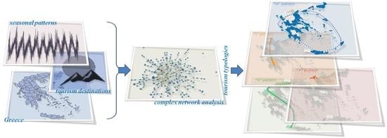
Detecting Tourism Typologies of Regional Destinations Based on Their Spatio-Temporal and Socioeconomic Performance: A Correlation-Based Complex Network Approach for the Case of Greece

by
Dimitrios Tsiotas
1,2,*,
Thomas Krabokoukis
3 and
Serafeim Polyzos
3
1
Department of Regional and Economic Development, Agricultural University of Athens, 118 55 Athens, Greece
2
School of Social Sciences, Hellenic Open University, 106 77 Athens, Greece
3
Department of Planning and Regional Development, University of Thessaly, 382 21 Volos, Greece
*
Author to whom correspondence should be addressed.
Submission received: 13 February 2021 / Accepted: 20 February 2021 / Published: 26 February 2021

Abstract

:
Within the context that tourism-seasonality is a composite phenomenon described by temporal, geographical, and socio-economic aspects, this article develops a multilevel method for studying time patterns of tourism-seasonality in conjunction with its spatial dimension and socio-economic dimension. The study aims to classify the temporal patterns of seasonality into regional groups and to configure distinguishable seasonal profiles facilitating tourism policy and development. The study applies a multilevel pattern recognition approach incorporating time-series assessment, correlation, and complex network analysis based on community detection with the use of the modularity optimization algorithm, on data of overnight-stays recorded for the time-period 1998–2018. The analysis reveals four groups of seasonality, which are described by distinct seasonal, geographical, and socio-economic profiles. Overall, the analysis supports multidisciplinary and synthetic research in the modeling of tourism research and promotes complex network analysis in the study of socio-economic systems, by providing insights into the physical conceptualization that the community detection based on the modularity optimization algorithm can enjoy to the real-world applications.

Graphical Abstract

1. Introduction

A variety of theories and models have been developed over time aiming to study the uneven developmental dynamics that emerge between regions and to contribute to the academic dialogue towards the direction of seeking a solution to the regional problem that concerns the reduction of spatial inequalities [1,2,3,4,5,6,7,8,9]. In general, the uneven spatial development affects the economic growth [2,3], the quality of the environment, the culture, and the social conceptualization [4,5,6], and, therefore, it can be considered as a major driver for the sustainable economic development [7,8]. This aspect highlights the importance of studying spatial inequalities in the research of regional economics [1,9], where tourism is a major field due to its socio-economic configuration that affects the regional, national, and worldwide economic interaction and thus the economic development [8,9,10]. Provided that tourism is a time-variant socio-economic phenomenon that is by default equipped with a spatial reference, the study of tourism within a common temporal and spatial context [6,7,8] can provide insights towards the demand for integration, which can contribute to the multidisciplinary conceptualization of regional economics [9,11]. Amongst the many others, a major property of tourism [12,13,14,15,16], which diversely affects almost every destination [9,17], is related to the phenomenon of (the so-called) tourism-seasonality, which concerns the uneven distribution of tourism-demand along the period of the year [6,18]. The nature of this phenomenon is rather complex, as it can be deduced first by the definition of this term, which is composed by the concepts of tourism demand [1,6,9,12,14,15,16,18], which is related to the intensity of the tourist load applied to a destination, time [1,6,9,11,12,15,17], which describes how tourism demand is distributed through time, and space [6,9,12,14,15,16,17,18], which describes those geographical features that link a destination with a specific pattern of seasonality. This 3D conceptualization allows considering corresponding spaces of embedding for the study of seasonality, such as the socioeconomic space, where social and market activities related to tourism demand are developed, the temporal space, which is the timeframe where socioeconomic forces evolve, and the geographical space, which is the spatial receptor where market activities apply throughout time. Based on this conceptualization, we construct Table A1 shown in the Appendix A, where modeling and implementation aspects of tourism seasonality extracted from the literature can be organized by these 3D conceptual approaches. This multi-block table reveals several aspects composing the complexity of tourism seasonality, which is related to diverse factors [18,19,20,21,22,23,24,25,26,27,28] that can be either environmental [6,14], such as the geomorphology and climate [18,19], or social [20], such as the synergy among the destinations [24,25,26] and the traditions [28,29], or geographical [9,25,30], such as the accessibility of destinations [25], or economic [1,9], such as the tourism-capacity [21], the competitiveness [22,23,27], the attractiveness of destinations [10], the configuration of local economies [15], and the type of tourism product [29] (see column B3, Table A1, Appendix A). As is evident in all such aspects of tourism-seasonality, the spatial dimension is an immanent (either directly or indirectly) in the conceptualization of the phenomenon [9].
However, in the current literature, the temporal dimension of tourism-seasonality is mainly examined [6,9] by using various methodologies that are applied within a certain geographical and socio-economic framework (column C1, Table A1, Appendix A) [9,14,31], but without considering how space affects the seasonality’s temporal dynamics. For instance, a major class of research-studies examines the temporal aspect of seasonality by mainly analyzing the time-series configuration of a specific variable, for a certain destination [14,15,32,33], without thus taking into account the variability in the seasonality’s temporal patterns that are caused by the location. In this class, the variables that are most commonly used are (column B2, Table A1, Appendix A) the number of tourists (visitors), arrivals, and overnight-stays, whereas also some income-defined variables are used [9,30,31]. This uni-variable approach (column B1, Table A1, Appendix A) is usually sensitive to the subjectivity in the variables’ selection [31] and to the sampling-rate, according to which the time-unit (e.g., months, days, etc.) is being defined [14,34]. On the other hand, another direction in the study of seasonality regards the computation of quantitative measures or indicators (column B4, Table A1, Appendix A) that are capable of capturing different aspects of this phenomenon (column B3, Table A1, Appendix A), such as concentration, scale, periodicity, or cyclical performance [9,35,36,37]. Some indicative measures of this category are the range of seasonality, the seasonality-ratio, the coefficient of variation (CV) and seasonal variation [35,36], the Gini coefficient, and the Theil index [9,37], some of which are rather useful due to their ability to decompose into components [38,39,40,41]. However, even in the most composite cases of these measures, such as in the case of the Gini coefficient and the Theil index, some critical information that is related to the seasonality (e.g., periodicity) can be lost [14,36] due to restrictions concerning either the data configuration (e.g., annual reference) or the spatial embedding of seasonality that is usually approximating by averaging techniques [15,39]. Some other more composite indicators that were recently proposed in the literature, such as the Relative Seasonal Index—RSI [14,36] and the synthetic DP2 index [31], promise to overcome these common restrictions describing the established indicators [9,14,36,42,43,44,45,46,47,48,49,50], but these composite indicators are also subjected to the restriction of uni-variable configuration and computational complexity due to higher demand in computations [9].
Despite that seasonality affects almost every tourism-destination (column C1, Table A1, Appendix A), in the current literature, the symbiotic relationship between seasonality and space does not seem to be studied in a comprehensive quantitative context. This observation is verified by the bi-dimensionality (column B1, Table A1, Appendix A) of the relevant research that was previously emerged [9], one pillar of which deals with the study of multivariate time (temporal) aspects of seasonality [6,14,17,30,31,32,33,45] that is mainly applied within the context of a single destination, whereas the second one, which studies geographical aspects of seasonality, overlooks the effect that time induces to the spatial patterns of tourism-demand [42,43]. Some bright exceptions to this dual conceptualization of seasonality can be found in the works of [4,5,6,9,17,44,49], which attempt to integrate the spatial and temporal dimension of this phenomenon through different methodological aspects, such as cluster analysis, econometric modeling, tourist area life cycle assessment, classification and dimension reduction modeling. However, such approaches rather highlight the demand for integration than adequately configure a comprehensive context for integrating the time (temporal) and geographical (spatial) dimensions of tourism-seasonality [9].
Aiming at serving the demand for integration, this paper proposes a new method for studying temporal patterns of tourism-seasonality in conjunction with their spatial information. The proposed method builds on a joint consideration of correlation and complex network analysis to convert into a complex network the temporal information of the seasonality patterns of the 51 (NUTS III) Greek regions, which are configured for the period 1998–2018, and then to classify these available patterns into communities, according to their level of connectivity in the network model. Complex network (or network) analysis is considered by many scholars as a separate discipline, called network science [51,52,53,54], uses the network paradigm to represent complex communication (or other interacting) systems as graphs, namely as pair-sets of nodes and edges that are converted into connectivity matrices, where many topological measures can be computed. In tourism research, network structures prevail [55,56,57,58] because tourism is by definition an act of interaction (or mobility) and thus the conceptualization of connectivity is by default applicable in the modeling of tourism systems. However, the network paradigm has not yet been sufficiently incorporated in tourism research and therefore there are many ongoing avenues of further research towards this direction [55,56,57]. For instance, a major benefit of the network conceptualization in the description of interconnected systems regards its ability to incorporate, within a single model, structural and functional (flow) information, at any scale (e.g., local, neighborhood, regional, or global), and thus to provide a dual microeconomic and macroeconomic description of real-world systems [58]. Within this context, this paper uses the network paradigm to model correlations between seasonality patterns as a complex network, which (according to the dual conceptualization of networks) allows incorporating topological information related to the connectivity of correlated data with the scale and variability information captured by correlation analysis. The study examines the case of Greece, which enjoys a considerable tourism specialization, where almost 20% of its GDP is related to direct tourism activities [46,47,48,49,50,51], it is a top-ranked in the EE27 in terms of the number of visitors [46], amongst which the 50–60% of foreign arrivals is implemented in the high-season period of July to September [47]. Greece has more than 16,000 km of coastline and more than 1350 islands, islets, and rocky-islands [47], and its rich geomorphological configuration has led to a composite tourism product [50], which is unevenly distributed throughout the various tourism-destinations of the country [49,50,51].
Within this context, the proposed methodological framework allows classifying the Greek prefectures according to their seasonality patterns, aiming to be insightful about the spatial configuration of tourism-seasonality in Greece and how it can be managed in conjunction with the dynamics of the regional space. The main research question addressed in this paper is configured within an exploratory context and it concerns whether temporal patterns of tourism seasonality can be related to the spatial distribution and the socioeconomic attributes of the regional destinations in Greece. The overall approach can drive to more efficient and sustainable management, planning, and hospitality strategies in tourism, which can contribute the Greek tourism-destinations to the goal of balanced regional development.
The rest of this paper is structured as follows: Section 2 describes the methodology of the study, the available data, and the variables that are included in the analysis. Section 3 shows the results of the analysis and provides a discussion within the context of tourism management and regional economics. Finally, in Section 4 the conclusions are summarized.

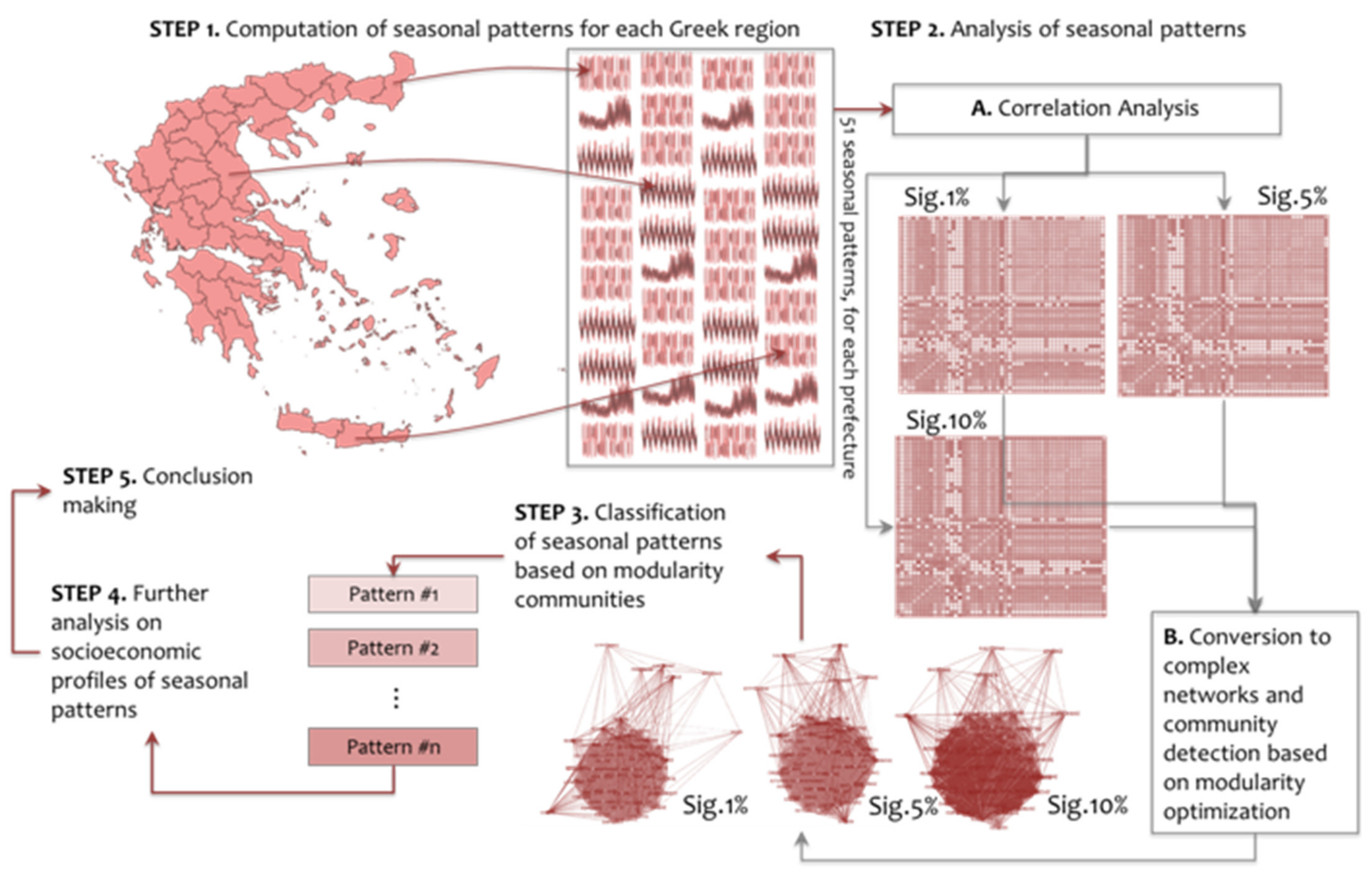
2. Methodology and Data

This study configures a methodological framework for analyzing temporal patterns of tourism-seasonality amongst the 51 Greek regions and for classifying them into regional groups, according to their relevance in connectivity that is defined after applying complex network analysis to the seasonal data. The purpose of the analysis is to detect linear and non-linear commonalities in the temporal patterns of tourism-seasonality of the Greek regions, to categorize them into groups, and to detect distinctive seasonal profiles. Towards this direction, the proposed methodology builds on complex network analysis [51,52,53,54] that is applied to the seasonal data after converting them to graphs through a correlation-based criterion. In particular, the methodological framework of the study consists of the five steps shown in Figure 1.
At the first step, the seasonality-variables expressing the seasonality patterns of the Greek prefectures are computed, on data expressing the monthly number of total overnight-stays per prefecture (NUTS III), which are recorded for the years from 1998 up to 2018. The available data were granted upon request by the Hellenic Statistical Authority [59] to be used under an exclusive license for this study. In particular, 51 seasonality-variables are configured, each one representing the time-series of the monthly overnight-stays recorded per prefecture (codes and variable-names are shown in Table A2, in the Appendix A).
At the second step, the seasonality-variables are first included in a correlation analysis, where the Pearson’s bivariate coefficients of correlations [60] are computed for all possible pairs of the available variables. The square table of correlation coefficients is then filtered according to the level of significance, where only significant coefficients are preserved. Therefore, for significances 1%, 5%, and 10%, this allows producing three correlation tables corresponding to a certain significance level. At next, each table is converted to a network (graph) model, each one expressing a weighted graph of 51 nodes, where the links have weights equal to the significant correlation coefficients, for this case.
Further, a community detection analysis [61] that builds on the modularity optimization algorithm of [62] is applied to each network model (corresponding to 1%, 5%, and 10% levels of significance). This algorithm generates communities by maximizing the intra-community connectivity (i.e., the connectivity of the nodes included within a community), which simultaneously minimizes the inter-community (i.e., between the communities) connectivity, as is described by the mathematical expression [61]:
maximize [Q ∝ (mwithin communitiesmbetween communities)]
where Q is the modularity-function [61] and m is the number of network edges (links). The community detection [61,62] is implemented through a greedy algorithm that is applied in two steps [54,61]. At the first step, all nodes in the graph are assigned to different communities. Afterward, the nodes are step-by-step being swept and placed into collective-communities if the assignment of a node into an adjacent community increases the weighted modularity function of the original model. At the second step, the collective-communities are replaced by new (super-) nodes, and the process is repeated up to the point that the modularity function cannot increase anymore [61]. Generally, greedy algorithms are sensitive to regional conditions, where the algorithm can be “trapped” in the area of a local-optimum and thus cannot move to a better (global) solution [54,61,62]. Therefore, the generated communities do not a priori describe the (globally) optimum partition of the graph-model into communities but a quite satisfactory division, which ensures that nodes within the communities are well-enough densely connected and well-enough sparsely connected between the communities. According to the comparison provided by the author of [61], amongst 12 in number modularity optimization algorithms, the algorithm of Blondel et al. [62], which is chosen in this paper to run the community detection analysis, belongs to the pair of cases with the smallest order of computational complexity O(m). This property gives this algorithm a privilege to be considered as one of those with optimum performance and, also, its availability to be built-in in the open-source software of [55] makes it a popular choice for community detection analysis. However, the community classification outcome is inevitably dependent on the algorithm that is chosen to perform the analysis, and therefore the results of the community detection cannot be considered unique. For a detailed review about community detection in networks and the optimization methods, the interested reader is referred to the reference work of [61]. Within this context, to manage the restriction due to the greedy architecture of the modularity optimization algorithm, which brings uncertainty both at the step of the algorithm’s choice (amongst several others) and at the step of applying the specific algorithm to the network dataset (where the initialization of the algorithm is by default submitted to randomness), we apply some repairing techniques, as follows: First, the community detection analysis is designed to be applied to three correlation-based complex networks (i.e., those converted at 0.01, 0.05, and 0.10 level of significance tables) instead of one, so that the final communities to result by the synthesis of these three aspects incorporating different levels of uncertainty and variability in network connectivity. Secondly, we run the procedure of community detection for a single significance-network several times and we then configure the final community outcome by the mode (i.e., most frequent solution) of all runs. Finally, the results of the analysis in this paper are compared with those obtained in previous work of [9], which applied a grouping to the available seasonal patterns of the Greek prefectures based on the principal components analysis method. Interpreting the results of the comparison in terms of regional dynamics and tourism development will provide an evaluation of the proposed in this paper methodology. All these three repairing approaches are expected to reduce the sensitivity of the modularity optimization algorithm due to its greedy architecture.
At the third step of the methodology, the different patterns referring to the modularity communities resulted for 1%, 5%, and 10% levels of significance are jointed to a single classification of seasonal modularity-patterns. This joint-classification takes into account the unique modularity-community patterns of the form (Q1%(i), Q5%(i), Q10%(i)), where each node (i) belongs to.
At the fourth step, the patterns resulted from the classification of the seasonality modularity-patterns are evaluated by their geographical and socio-economic features that are approximated by a set of 51 variables, as shown in Table A3 in the Appendix A. This analysis is based on the formulation of error-bars expressing 95% confidence-intervals (CIs), which are computed for the mean values [54,60] of the available socio-economic and geographical (SEG) variables amongst the groups referring to the available seasonal modularity-patterns. When the error-bars do not overlay, the mean values referring to modularity-groups are considered as statistically different, under a 95% certainty [9,54,60]. Thus, comparisons amongst the modularity-groups applied for every SEG variable (Table A2, Appendix A) can reveal which group outperforms (i.e., has a maximum performance) or underperforms (i.e., has a minimum performance) in terms of a single SEG attribute. Within this context, the comparison-results are further tabulated to formulate the total profiles (including seasonality, socio-economic, and geographical information) of the available modularity-groups [9]. This part of the analysis develops linkages between the temporal (as expressed by the time-series patterns of overnight-stays on which the analysis is built), socio-economic, and geographical dimension in the analysis of tourism-seasonality and thus to contribute to the conceptualization of integrating modeling of the complex phenomenon of tourism-seasonality.
The overall approach provides a tool of quantitative analysis that can be proven useful for the scholars and practitioners activating on regional planning, tourism policy, and hospitality management. The findings and the results of the analysis are discussed at the fifth step of the methodology, where an overall assessment and conclusions are formulated.

3. Results and Discussion

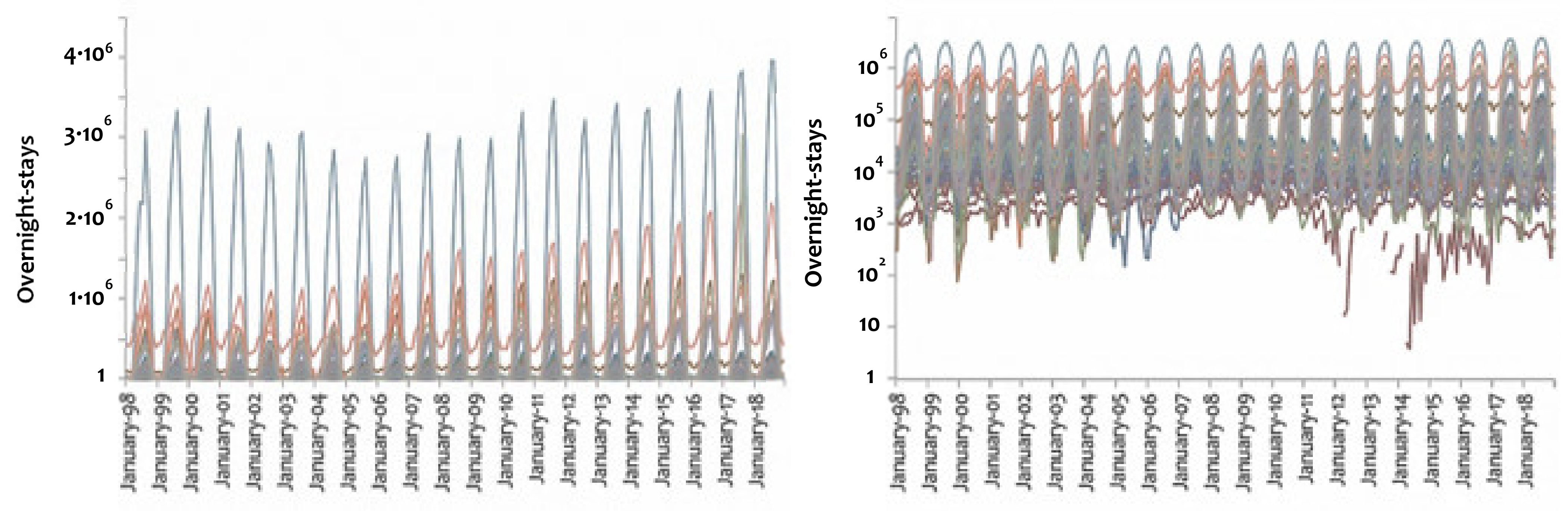
3.1. Data Visualization

The available 51 seasonality-variables of overnight-stays participating in the analysis are first presented to the diagrams shown in Figure 2. This is done for visually detecting possible similarities amongst the seasonality patterns of the 51 Greek prefectures. Each seasonality-variable refers to a Greek region (prefecture) and has 252 monthly records of tourism overnight-stays (i.e., is of length 252), which are recorded for the period from January 1998 to December 2018 [59]. As is evident, almost all available variables have a distinguishable periodicity, which is evident by the oscillating curves of the line-plots. In these patterns, differences in scale (i.e., the oscillation height) and in trend (e.g., some seasonality patterns are described by an increasing trend) can be observed, which are more distinguishable in the metric rather than in the semi-log scale. In particular, in the metric representation, three scale-levels (zones) can be observed in the overlaid line plots of Figure 2, where approximately the first zone ranges from 0–500,000, the second one from 500,000–2 million, and the third one from 2–4 million (measured in overnight-stays). These levels correspond to different oscillation heights that express different levels of magnitude in tourism overnight-stays. However, in the semi-log representation, these zones observed in the metric scale do not seem to propose a distinguishable grouping, similarly to the metric case. Instead, in the semi-log scale, one concentration of “noisy” (i.e., not following clear periodical) patterns can be observed at the range of 10–20,000, another cluster of distinguishable periodical patterns can be observed at the range of 100–1 million, and a final one at the range of 100,000–3 million (all expressing overnight-stays).
The previous visual examination of the available data’s time-series curves indicates that pattern recognition on data that are jointly submitted to the temporal and geographical configuration is a task of high complexity, where supervision based on intuition can be easily lost, especially on big datasets. Within this context, this paper applies a multi-level approach based on correlation and complex network analysis to jointly manage the temporal and spatial information describing the available dataset. This multi-level approach deals with complexity by integrating linear and non-linear methods and aims to contribute to pattern recognition in seasonality and generally in tourism research.

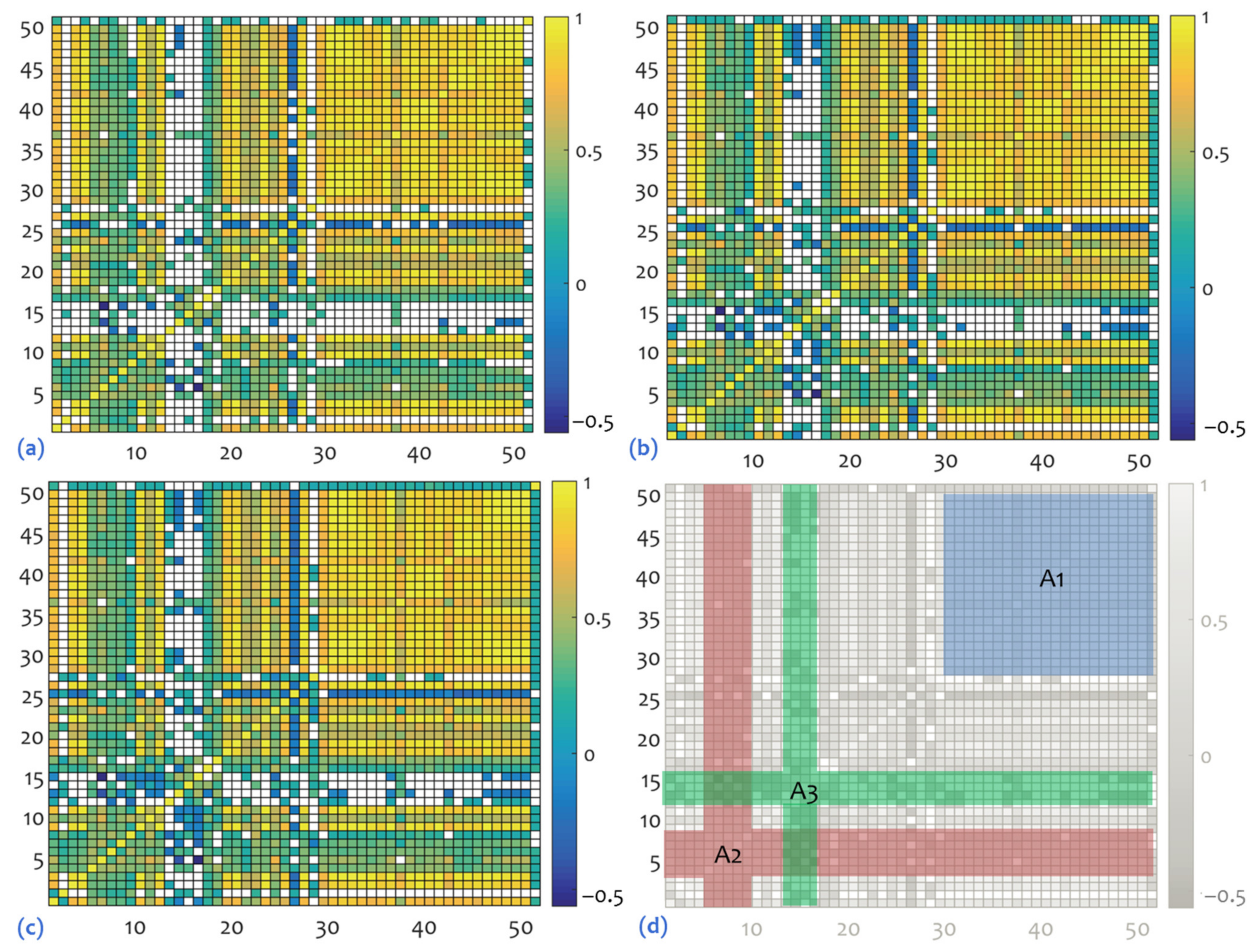
3.2. Correlation Analysis

In the second step of the analysis, the seasonality-variables participate in a correlation analysis to detect linear relations between the possible variable pairs. The results of the analysis are shown in Figure 3, where the correlation tables for each level of significance (i.e., 1%, 5%, and 10%) are illustrated in heat-maps. In all cases of significance, the analysis first illustrates a distinguishable sub-table {29:50} × {29:50} of high positive correlations (>0.6), which is shown as area A1 in Figure 3 and is configured by the rows 29:50 and the lines 29:50. This sub-table (A1) includes the seasonality patterns of the prefectures of Fokida (29), at central Greece, Kerkyra (30), Zakeenthos (31), Kefalonia (32), and Lefkada (33), at the Ionian Sea (west Greece), Achaia (34), Aitoloakarnania (35), and Heleia (36), at west Greece, Arkadia (37), Argolida (38), Korinthia (39), Lakonia (40), and Messenia (41), at the Peloponnese, Attiki (42), which is the metropolitan prefecture of Greece, Lesvos (43), Samos (44), Chios (45), Cyclades (46), and Dodecanese (47), at the Aegean Sea, and Heraklion (48), Lasithi (49), and Rethymno (50), on the island of Crete. As it can be observed in Figure 4, the geographical arrangement of these regions is based on the state of the adjacency (where prefectures are mainly located in central and south Greece), have geographical relevance, and their spatial distribution configures a "U"-shaped pattern.
Another distinguishable area that can be observed in Figure 3 is the cross-junction area A2, which includes the seasonality patterns of the prefectures of Xanthi (5), Thessaloniki (6), Hmathia (7), Kilkis (8), and Pella (9). All these regions have geographical relevance, as they are located in north-east Greece (Figure 4), as well as tourism-seasonality (functional) relevance, to the extent that they are in their majority positively correlated to all the other seasonality patterns of the Greek regions. A final distinguishable area that can be observed in Figure 3 is the cross-junction area A3, which includes the seasonality patterns of the neighbor prefectures of Kozani (13), Grevena (14), Kastoria (15), and Florina (16). These regions have also geographical relevance due to their neighboring location in north Greece (Figure 4) and their functional relevance regards their either negative or insignificant correlations to all other seasonality patterns of the Greek regions.

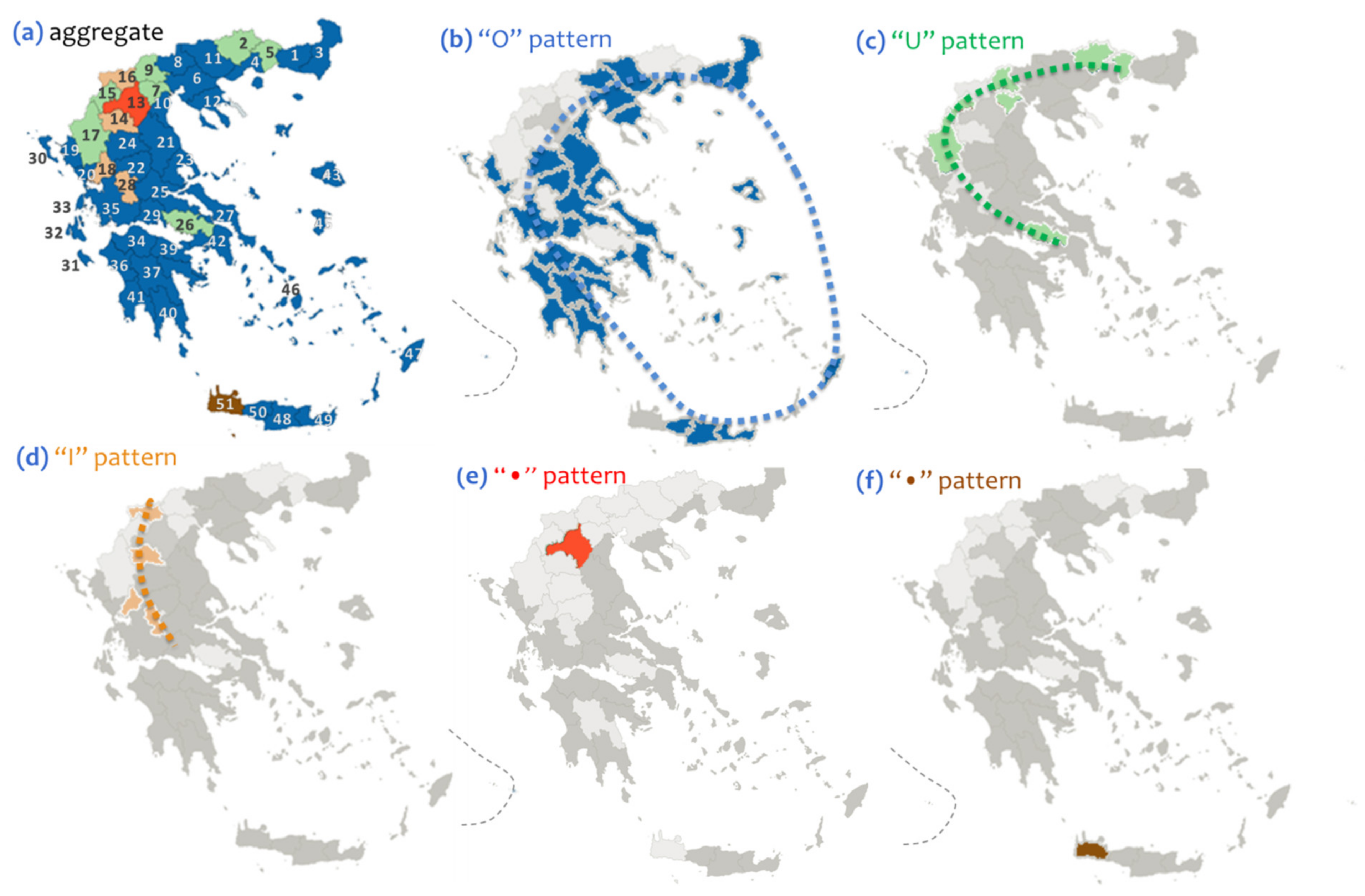
3.3. Classification of Seasonality Patterns Based on Community Detection

As being evident by the previous correlation analysis, the temporal dimension of tourism-seasonality can enjoy a spatial conceptualization, which is expressed by the state of neighborhood or adjacency amongst regions with correlated seasonality patterns. However, pattern recognition based exclusively on correlation analysis cannot be that insightful because the geographical patterns that emerged by correlations are quite primary and selective, to the extent that they do not include the total cases of the available population. Within this context, the correlation tables of Figure 3 are converted to graph-models, where a link expresses the value of a significant correlation coefficient between two nodes (prefectures). These graph-models are afterward divided into communities, by applying the modularity optimization algorithm [54,61,62], which generates communities with dense connectivity within and sparse connectivity between them.
The results of the community detection are shown in Figure 5, where regions are colored according to the community they belong to. As it can be observed, for the 1% and 5% level of significance the graph-models are divided into 3 communities, whereas for the 10% level of significance the graph-models are divided into 2 communities. Communities for the graph-models of 1% and 5% levels of significance include the same number of members, the first one consisting of 13 prefectures, the second one of 6, and the third (and bigger) one of 32 elements. On the other hand, the first community for the graph-model corresponding to the 10% level of significance includes 18 members (prefectures), whereas the second one includes 33 elements. As it can be observed, the community grouping corresponding to the case of 10% significance level results by merging the 13-element and 6-element communities of the 1% and 5% significance levels and by shifting one element, the prefecture of Kozani (13), to the 32-element community of the 1% and 5% significance levels. This observation implies first that the 13-element and 6-element communities of the 1% and 5% significance levels become relevant when uncertainty increases (and thus they are linked in a weak-ties context) and secondly that the prefecture of Kozani (13), shows an interesting outlier performance due to its community shift, suggesting a special case to study.
To evaluate the information provided by the community detection of the available (interregional seasonal correlation) graph-models and to manage the results of the community detection algorithm within a context of repairing their heuristic configuration, a joint assessment is applied to the available modularity classes (communities). In particular, based on the modularity class that each prefecture belongs to, we construct ordered triplets of the form p = (p1,p2,p3), where the first coordinate (p1,,) expresses the modularity class for the 1% level of significance, the second one (,p2,) for 5% sig., and the third one (,,p3) for 10% significance. Therefore, based on the available ordered triplets p(i), which correspond to the i = 1,…, 51 modularity (seasonal) classes of the Greek prefectures, four (4) in number unique patterns (clusters) can be distinguished, which are expressed by the triplet-groups (0,0,1), (1,1,0), (1,1,1), and (2,2,0), as is shown in Figure 5. Amongst these patterns (clusters) of modularity classes, the first one configures a sigmoid (“S”-shaped) spatial pattern (Figure 6b) that consists of the prefectures of Drama (2), Xanthi (5), Thessaloniki (6), Imathia (7), Kilkis (8), Pella (9), Serres (11), Kastoria (15), Ioannina (17), at northern Greece, the prefectures of Karditsa (22), Trikala (24), and Viotia (26), at central Greece, and Chania (51), at the island of Crete. The second one includes a single prefecture, Kozani (13), which is located in north Greece (Figure 5 and Figure 6) and thus it configures a point or dot (“•”-shaped) spatial pattern (Figure 6c) at the central Macedonia region. As is evident, this community consists of the single element with the most unstable connectivity, as denoted by the shifting captured by the intersection consideration of communities between the 1%, 5%, and 10% significance levels. The third cluster configures a linear spatial pattern (Figure 6d) consisting of the prefectures of Grevena (14), Florina (16), at north Greece, Arta (18) and Evrytania (28), at central Greece, and the prefecture of Arkadia (37), at the region of Peloponnesus.
Finally, the fourth cluster configures a circular (“O”-shaped) spatial pattern (Figure 6e) that consists of the prefectures of Rodoph (1), Evros (3), Kavala (4), and Chalkedikh (19), at the regions of eastern Macedonia and Thrace, Pieria (10), Thespotia (12), Preveza (21), Aitoloakarnania (35), Kerkyra (30), Zakeenthos (31), Kefallonia (32), and Lefkada (33), at west Greece, Larissa (21), Magnessia (23), Ftheotida (25), Euvoia (27), and Fokeeda (29), at central Greece, Achaia (34), Heleia (36), Argoleeda (38), Korenthia (39), Lakonia (40), and Messeenia (41), at the region of Peloponnesus, the metropolitan region of Attiki (42), Lesvos (43), Samos (44), Chios (45), Keeklades (46), and Dodekaneese (47), at the Aegean Sea, and Herakleeo (48), Lasithi (49), Rethymno (50), at the island of Crete.
According to the community detection analysis, the modularity communities can relate the temporal with the spatial dimension of tourism-seasonality within a more perplexing context than this shown in Figure 4, where the modularity groups (p1, p2, p3) that were generated configure diverse but also distinguishable spatial patterns in the geographical map of Figure 6. Within this framework of complexity, to further decompose and examine the multiplex information included in these modularity groups, we illustrate the line-plots of the overnight stay time-series per modularity group, as is shown in Figure 7. As it can be observed, modularity groups (0,0,1) and cluster (2,2,0) include seasonality patterns with more discrete periodical patterns, whereas groups (1,1,0) and (1,1,1) are described as more noisy patterns. In particular, the first modularity group (0,0,1), which corresponds to the “S”-shaped spatial pattern of Figure 6, includes cases that are described by a periodic pattern with an increasing trend. The case included in the second modularity group (1,1,0), which refers to the “dot”-shaped spatial pattern of Figure 6, is described by a noisy seasonal pattern with a decreasing trend, where linearity is more obvious in the time-series curve than periodicity. Also, the third modularity group (1,1,1), which corresponds to the "I"-shaped spatial pattern of Figure 6, includes cases that are described by a noisy periodical pattern that configures (on average) a bell-shaped curve with its convex part defined at the period 2003–2012. Finally, the fourth (and larger) modularity group (2,2,0), which corresponds to the “O”-shaped spatial pattern of Figure 6, includes cases that are described by an approximately cyclical pattern (i.e., a periodical with the same oscillation amplitude) that configures (on average) a U-shaped curve with its concave part also defined at the period 2003–2012. Overall, this analysis allows claiming that the four available modularity groups have, along with their spatial patterns, distinguishable seasonality patterns, on average.
To detect differences at the scale of seasonality amongst the available modularity groups, we apply further analysis based on error-bars of confidence intervals (CIs) [54,60]. In particular, we construct 95% CIs for the mean values of the Gini coefficient [9,37] and the RSI (Relative Seasonal Index) [14,36], which are composite indicators capturing aspects of seasonality on a set of data. The results are shown in Figure 8, where it can be observed that the modularity group (2,2,0), the one with the “O”-shaped spatial pattern, has on average the maximum score of seasonality, which is statistically different than these of all the other groups. On the other hand, the modularity group (1,1,0), described by the “dot”-shaped spatial pattern, has on average the minimum score of seasonality, which is statistically different than this of (1,1,0) and (2,2,0) groups. However, no statistical difference can be detected between the (0,0,1) and (1,1,1) groups, implying that their seasonality patterns lie on the same scale level. Overall, this analysis highlights that community detection resulted from the modularity optimization algorithm sufficed to configure communities separating the minimum and maximum performance in tourism-seasonality, as it can be captured by the Gini coefficient and the Relative Seasonal Index.

3.4. Socio-Economic Determination of the Modularity Seasonal Groups

In the fourth step of the methodology, the available modularity groups are interpreted in terms of their geographical and socio-economic information. To do so, the analysis builds on comparisons amongst error-bars of 95% confidence intervals, which are computed for a set of 51 (in number) available variables that are divided into thematic categories (geographical, seasonality, transport, demographic, productivity, tourism, environmental, and cultural), as is shown in the Appendix A (Table A3). Based on the error-bars comparisons, the statistically significant minimum and maximum performances per variable are tabulated and shown in the Appendix A (Table A4). According to this analysis, the prefectures belonging to the modularity group (0,0,1) have high urbanization, winter tourism activity specialization, the capacity of "Natura" (i.e., biodiversity protected) areas, and the capacity of woodland parks. On the other hand, the prefectures included in this group have not rich geomorphological configuration, relatively low seasonality performance, and a small number of ports, are not specialized in the secondary sector, not equipped with industrial areas, and have a small number of camping areas and beaches. The prefecture of Kozani (13), which configures the modularity group (1,1,0), is located in northwest Greece, is a mainland prefecture with rich geomorphological configuration, high income, tourism specialization, and specialization in winter tourism activities.
On the other hand, this single-member group has low seasonality, tourism capacity in terms of accommodation, and level of environmental and cultural resources. The prefectures belonging to the modularity group (1,1,1), which are mainly located on the mainland, are cases with high urbanization, but with low geomorphological configuration, seasonality, sea geomorphology, and tourism profile, as well as demographic and income background. Finally, the prefectures belonging to the modularity group (2,2,0) are mainly located in southeast Greece, where their sea geomorphologic configuration is dominant. Prefectures of this group have high seasonality, urbanization, primary and tertiary sector specialization, tourism profile, and environmental and cultural resources. On the contrary, cases of this modularity group have low mountainous geomorphology. All previous interpretation is tabulated in Table 1, where the socio-economic and geographical profiles of the modularity groups are illustrated.
As it can be observed from Table 1, the first modularity group (0,0,1), which is a group with a sigmoid geographical distribution and a seasonal pattern described by periodicity and an increasing trend, is a group where its relatively low seasonality pattern seems to be driven by forces related to winter tourism activities and MICE tourism (i.e., meetings, incentives, conferencing, exhibitions) attractions due to urbanization configuration. The second modularity group (1,1,0), concerning a single-prefecture group described by a noisy low seasonality pattern with a decreasing trend, has its seasonality related to the mainland geomorphology, high rail, and airport integration (but poor road density), and a mountainous tourism specialization. The third modularity group (1,1,1), which configures a linear geographical pattern and has a noisy periodical pattern with a bell-shaped curve running a stage of decline, is a group owing to its seasonal pattern to high environmental wealth and forces related to tertiary specialization and low transport integration and tourism profile. Finally, the fourth modularity group (2,2,0), which is the largest group described by a circular geographical configuration and an approximately cyclical pattern of seasonality, has its seasonality related to its rich sea geomorphology, environmental, and cultural wealth, as long as transport integration. This group is mainly related to the 3S (i.e., sea, sun, and sand) tourism activities that are the dominant model describing the nature of the tourism product in Greece.

4. Further Analysis and Overall Assessment

To further evaluate the effectiveness of the overall correlation-based complex network analysis applied in this paper, we compare the results of the modularity grouping with those presented in a previous work [9] of the authors, which were produced by applying a Principal Components Analysis (PCA) method to the same overnight-stays database. This comparative approach, on the one hand, is expected to provide insights into the uncertainty due to the modularity optimization algorithm and, on the other hand, to evaluate the effectiveness of the method proposed in this paper. In particular, the authors of [9] applied a PCA to the same set of seasonality-variables (see Table A2 Appendix A) by choosing the covariance matrix extraction and the Varimax rotation methods. The PCA resulted in seven (7) principal components explaining a high percentage (84.86%) of the total variance. Provided that the PCA’s component matrix includes component loadings (which are defined by correlations) between the principal components and all the available variables, further min-max filtering was applied in this approach to singularly assign one variable in a unique PCA component. The PCA yielded two groupings of the available 51 Greek prefectures, where the first one (which was generated by considering only the maximum -M- component loadings per variable) consisted of five (5) groups including 38 (PCM#1), 7 (PCM#2), 4 (PCM#3), 1 (PCM#4), and 1 (PCM#5) cases (prefectures) respectively, while the second one (which was generated by considering only the minimum -m- component loadings per variable) consisted of seven (7) groups including 1 (PC#1), 7 (PC#2), 13 (PC#3), 14 (PC#4), 8 (PC#5), 5 (PC#6), and 3 (PC#7) cases, respectively. The labeling of both PCA groupings was according to the ranking of the principal components resulted from their eigenvalues shown in the scree plot.
Within this context, Table 2 is constructed for the comparison and measurement of the relevance between the modularity grouping (MOD) applied to this paper with the PCA grouping applied in the previous paper [9] of the same authors. This comparison table has a multilayer block-structure consisting of a window (block) named "Intersection Frequencies" that displays the set-theoretic intersections P C # i M O D # j between the i-th PCA and j-th modularity groups, two other blocks named “Relevance to PCA/MOD Groups” that display the percentage (%) of coverage that the PCA/MOD groups have for each intersection, and a final window displaying relevance differences that imply which (PCA/MOD) group is more relevant (dominant) to each intersection.
As it can be observed, first the PCM grouping (which is generated by the max-filtering of the PCA component loadings) includes 4 intersections equal to entire PCM groups, which are the groups P C M # 2 0 , 0 , 1 = PCM#2, P C M # 3 1 , 1 , 1 = PCM#3, P C M # 4 1 , 1 , 0 = PCM#4, and P C M # 5 0 , 0 , 1 = PCM#5 consisting of 13 prefectures in total. Next, the PCm grouping (which is generated by the min-filtering of the PCA component loadings) does not include intersections equal to entire PCm groups P C M # i M O D # j ≠ PCM#i. Finally, the MOD grouping applied to this paper includes 2 intersections equal to entire MOD groups, namely P C M # 1 2 , 2 , 0 = (2,2,0) and P C M # 4 1 , 1 , 0 = (1,1,0), which include 33 cases in total. This observation implies a better performance of the modularity than the PCA grouping because the intersections that equal to entire MOD groups are bigger in the total group size.
Next, according to the relevance-assessment shown in Table 2, the 6 cases (prefectures) composing the complementary set C#1 = PCM#1− P C M # 1 2 , 2 , 0 participate in an amount of 38.5% in the configuration of the modularity group (0,0,1), 20% in the configuration of the modularity group (1,1,1), and 13.2 + 2.6 = 15.8% in the configuration of the PCM#1 group. These shares imply that set C#1 is more relevant in the configuration of the modularity than the PCA groups and therefore they can provide another indication of better performance of the MOD than the PCA grouping.
Finally, as is evident by the block-structure of Table 2, the PCA grouping is by default described by a higher level of complexity than the MOD grouping because of the dual (min-filtering and max-filtering) structure describing the PCA groups. Therefore, in terms of resolution of the grouping outcome, the modularity grouping can be considered more reliable than the PCA’s because it results in a singular instead of dual grouping outcome. Moreover, amongst the two PCM and PCm groups, the modularity grouping appears more relevant to the max-filtering (PCM) than to the min-filtering (PCm) outcome. This relevance is obvious in terms of groups’ number (i.e., the number of MOD groups is closer to the number of PCM than PCm groups), but it can be further supported by the rank-size distribution of the groups, which follows a power-law pattern in the case of PCM and MOD groupings whereas a Gaussian-like for the PCm grouping.
In spatial terms, Figure 9 and Figure 10 show the geographical distribution of the max-filtering (PCM) and min-filtering (PCm) groupings resulted from the Principal Components Analysis being available in the previous work of [9]. As it can be observed in Figure 9, group PCM#1 configures an “O”-shaped pattern, PCM#2 a “U”-shaped pattern, PCM#3 an “I”-shaped, and PCM#4 and PCM#5 “dot”-shaped patterns. On the other hand, group PCm#1 configures a “dot”-shaped pattern, PCM#2 an “O”-shaped pattern, PCM#3 and PCM#4 “U”-shaped patterns, PCM#5 an “S”-shaped pattern, and PCM#6 and PCM#7 “I”-shaped patterns, as is shown in Figure 10. Between the PCM and PCm groupings, the geographical distribution of the former appears more relevant to this of the MOD grouping, whereas PCm appears less relevant and messier. On the one hand, this relevance (that is observed between the spatial patterns of the PCM and MOD groupings) is consistent with the quantification shown in Table 2 and generally implies that different clustering techniques can lead to converging outcomes when the system being examined is described by considerable underlying causality. On the other hand, measurable differences that are captured between different grouping outcomes can quantify the reliability of each clustering technique. Within this context, the modularity grouping proposed in this paper appears overall more reliable than the PCA, in terms of grouping singularity, size, and configuration. This added value can be due to the complex-network approach applied in this paper, which incorporates topological information related to connectivity of interconnected data instead of just considering their scale and variability.
However, despite these indications of better performance describing the proposed complex-network-based method in comparison to the PCA grouping, a study that builds on clustering, numerical analysis, and heuristic optimization is inevitably submitted to uncertainty due to the modeling choices and computational constraints. In this paper, the number and the configuration of the generated groups were a result of optimization based on a heuristic algorithm, where iteration suggests a prime repairing technique to consider and manage the variability of results. Towards this direction, several avenues of further research can emerge. One may concern examining the convergence of the results due to iterations implemented within a single grouping method, such as the modularity grouping proposed in this paper. In this avenue, the characteristic parameters (e.g., degrees of freedom, variability, scale, etc.) describing the dataset and those describing the grouping outcome (e.g., number, scale, and variability of groups) can be correlated. Another avenue is examining the convergence between different grouping methods, similarly to the comparisons between the MOD and PCA groupings applied in this paper. In this approach, the variability observed in the grouping results (e.g., in the number and size of groups) should be evaluated in the light of the computational mechanism describing each method, which can be based either on variance, or distance, or scale, or positioning, or similar relevance-like conceptualization. Despite such computational-based approaches, avenues for further research can also emerge at the level of implementation, and particularly they can concern the management of the resulting groups in terms of tourism policy and regional development. For instance, an effective clustering on temporal patterns of tourism demand can be insightful for the tourism policy-makers to better distribute the national budget of tourism development across the regions based on their relevant profiles or to develop more efficient tourism developmental strategies that would be customized to the tourism profile of each group. Overall, the limitations that are applicable in this study can excellently suggest avenues of further research that can contribute to the integration of the spatial, temporal, and socioeconomic aspects in tourism research.

5. Conclusions

This paper developed a multilevel methodology for analyzing time (temporal) patterns of tourism-seasonality and for grouping them into regional classes and therefore to configure distinguishable seasonality profiles facilitating tourism policy and development. The proposed method was built on a multilevel pattern recognition incorporating time-series assessment, correlation (linear assessment), and complex network analysis (non-linear assessment) to deal jointly with the temporal and spatial dimension of tourism-seasonality and to interpret the results of the analysis in socio-economic terms. The available data were registrations of overnight-stays for the years from 1998 up to 2018, which were provided by the Hellenic Statistical Authority [59] under an exclusive license. The analysis revealed four groups of seasonality, which were configured by a connectivity conceptualization based on the modularity optimization algorithm, where each group showed to be described by distinguishable spatial and seasonality patterns and to enjoy distinct socio-economic semiology. In particular, the first modularity group has a relatively low seasonality, with a pattern described on average by periodicity and an increasing trend, and a sigmoid geographical distribution. The seasonal pattern of this group is driven by forces related to winter tourism activities and MICE tourism attractions. The second, single-prefecture, modularity group has the lowest seasonality and is described by a noisy pattern with a decreasing trend, where its seasonality is related to rich geomorphological mountainous configuration and a mountainous tourism specialization. The third modularity group has a relatively low seasonality with a pattern described by a linear geographical distribution and on average by a noisy periodical configuration with bell-shaped time evolution. The seasonal pattern of this group is driven by forces related to high environmental wealth and tertiary specialization but low transport integration and tourism profile. Finally, the fourth and largest in size modularity group has the highest seasonality, with a pattern described on average by an approximately cyclical pattern and a circular geographical configuration. The seasonal pattern of this group is driven by forces related to rich sea geomorphology, environmental and cultural wealth, and transport integration, all of which describe the dominant 3S model of the tourism product in Greece. Overall, the analysis supports multidisciplinary and synthetic research in the modeling of tourism-seasonality, which is a composite socio-economic phenomenon of high complexity, and also promotes complex network analysis in the study of socio-economic systems by providing insights into the physical conceptualization of community detection in real-world applications.

Author Contributions

Conceptualization, D.T.; Methodology, D.T.; Software, D.T. and T.K.; Validation, D.T., T.K. and S.P.; Formal Analysis, D.T., T.K. and S.P.; Investigation, D.T., T.K. and S.P.; Resources, D.T., T.K. and S.P.; Data Curation, T.K.; Writing—Original Draft Preparation, D.T. and T.K.; Writing—Review & Editing, D.T., T.K. and S.P.; Visualization, D.T. and T.K.; Supervision, D.T. and S.P. All authors have read and agreed to the published version of the manuscript.

Funding

This research is co-financed by Greece and the European Union (European Social Fund—ESF) through the Operational Programme “Human Resources Development, Education and Lifelong Learning 2014–2020” in the context of the project “Analysis and methodological approach of tourism-seasonality for the Greek regions” (MIS 5048961).

Data Availability Statement

Data are available within the main text and Appendix A.

Acknowledgments

The authors thank the anonymous reviewers for their valuable comments that significantly improved the quality of the paper.

Conflicts of Interest

The authors declare no conflict of interest.

Appendix A

Table A1. Literature table showing major conceptual aspects of tourism seasonality.
TOURISM SEASONALITY
A. CONCEPTUALIZATIONB. MODELINGC. IMPLEMENTATION
A1. DefinitionA2. Space of EmbeddingB1. Variable ComplexityB2. DataB3. Attribute/AspectB4. ModelsB5. ApproachC1. Geographical Scale
1. Tourism Demand [1,6,9,12,14,15,16,18,20,21,22,28,30,31,32,34,37,38,39,40,41,44,45],1. Socioeconomic [1,9,12,15,16,17,18,20,21,22,28,32,37,41,42,44,45]1. Uni-variable (one attribute) [6,14,32,33,40,41,43,45]1. Visitors [6,22,30,31,34,39]1. Concentration [9,39,40,42,45]1. Indicators [6,12,14,18,19,22,28,29,30,31,32,34,35,36,38,39,40,41,45]1. Single discipline [6,12,13,14,29,30,31,32,35,38,39,40,41,42,43]
2. Multivariable (many attributes) [9,15,16,20,21,22,28,31,34]2. Arrivals [13,15,16,32,33,34,41,42]2. Synergy [5] 2. Measures/metrics [9,14,21,31,36,40,43]2.Multidisciplinary [9,15,16,17,21,22,28,33,34,44,45]
3. Overnight-stays [9,12,14,17,18,29,31,32,36,38,40,45]3. Traditions [4,6,12,18]3. Econometric [15,17,21,22,44,45]
4. Income [16]. 4. Tourism-capacity [42].
5. Occupancy [12,16,17,18,31,35]5. Competitiveness [22,23,32,42]
6. Number of trips [28]6. Attractiveness [19,29,44]
7. Staff [31,45]7. Economic structure/configuration [15,44,45]
8. Prices [31] 8. Type of tourism product [6,12,17,18,28,30,31,32,35,37,39,40,44]
2. Time References [1,6,9,11,12,15,17,20,27,29,33,35,40,43,45]2. Temporal (time dimension) [9,13,18,29,33,34,35,38,39,41]1. Uni-variable [13,29,35,38,39]9. Daily [34,35,41] 9. Scale [4,5,17,27,36,40]4. Measures/metrics [5,13,35,36]1. Single discipline [6,12,29,35,38,39,40,43]
10. Weekly [34,41,43] 10.Variability [4,5,15,28,35,36,41]5. Time-series [9,13,29,33,35]
11. Monthly [6,9,12,13,15,16,18,28,29,30,31,33,35,38,39,40,41,43,45]11. Periodicity [4,13,15,35,36,38,40,41]6. TALC [42,49].2. Multidisciplinary [9,15,17,33,45]
12.Annual [14,19,21,35,40]12. Cyclical performance [9,14,29,35,36]7. Pattern recognition [9,29,35,36,38,39]
3. Spatial References [6,9,12,14,15,16,17,18,19,20,21,25,28,30,32,34,37,39,40,42,43]3. Geography (spatial dimension) [9,12,14,15,16,17,18,19,29,31,34,40,42,43]1. Uni-variable (one destination) [12,18,30,32,33,34,35,41]13. Location [12,13,18,21,30,32,34,35,41,42]13. Geographical scale [6,9,19,28,42,44]7. Pattern recognition [12,14,18,42]1. Single discipline [6,12,14,29,30,39,40,42,43]1. Local [13,17,21,30,32,34,35,41,42]
2. Multivariable (many destinations) [6,9,14,15,16,17,19,28,34,36,38,39,40,43,44,45]14. Destination [9,14,15,16,17,22,28,31,33,34,36,38,41,42,43,44,45]14. Geomorphology [9,16]8. Classification [6,9,14,19,22,44]2. Multidisciplinary [9,15,16,17,21,28,34]2.Urban [34]
3. Climate [15,16],19]3. Regional [6,9,16,19,28,29,31,34,38,39,40,43,44,45]
15. Accessibility [16,30]4. National [12,18,22,33,34,40]
5. International [14,15,36]
Table A2. The seasonality variables participating in the analysis and correspond to the 51 Greek prefectures.
PrefectureVariable CodePrefectureVariable CodePrefectureVariable CodePrefectureVariable Code
ACHAIA34EVROS3KEFALONIA32PIERIA10
AITOLOAKARNANIA35EVRYTANIA28KERKYRA30PREVEZA20
ARGOLIDA38FLORINA16KILKIS8RETHYMNO50
ARKADIA37FOKIDA29KORINTHIA39RODOPI1
ARTA18FTHIOTIDA25KOZANI13SAMOS44
ATTIKI42GREVENA14LAKONIA40SERRES11
CHALKIDIKI12HELEIA36LARISSA21THESPOTIA19
CHANIA51HERAKLION48LASITHI49THESSALONIKI6
CHIOS45HMATHIA7LEFKADA33TRIKALA24
CYCLADES46IOANNINA17LESVOS43VIOTIA26
DODECANESE47KARDITSA22MAGNESIA23XANTHI5
DRAMA2KASTORIA15MESSENIA41ZAKEENTHOS31
EVIA27KAVALA4PELLA9
Table A3. The socio-economic and geographical (SEG) variables * used to determine the socio-economic profiles of the modularity groups of Figure 5.
CodeVariable’s SymbolDescriptionSource
SEG.1LATLatitude, defined by the geographical center of the prefecture.[63]
SEG.2LONGLongitude, defined by the geographical center of the prefecture.[63]
SEG.3RSIThe Relative Seasonality Index of the prefectures’ seasonality patterns[9]
SEG.4GINIThe Gini coefficient of the prefectures’ seasonality patterns[9]
SEG.5ROAD DENSITYThe road density (road length/area) of each prefecture (measured in km/km2).[64,65,66,67,68]
SEG.6ROAD LENGTHThe road length of each prefecture (measured in km).[64,65,66,67,68]
SEG.7COASTALDummy variable capturing coastal configuration (1 = coastal perfectures; 0 = non-coastal perfectures).[67]
SEG.8ISLANDDummy variable capturing island configuration.[59]
SEG.9INLANDDummy variable capturing inland configuration.[59]
SEG.10RAILThe length of the rail network.[48,68]
SEG.11PORTSThe number of ports.[59,68]
SEG.12AIRPORTSThe number of airports.[59,68]
SEG.13AREAThe geographical area (measured in km2).[59]
SEG.14POPThe regional population (2011 national census).[65]
SEG.15URBThe urbanization level (i.e., the proportion of the capital city’s population to the regional population).[65]
SEG.16GDPGross Domestic Product.[65]
SEG.17Human CapitalDefined by the proportion of labor-force (i.e., population between 18 and 65 years old) to the total population.[1]
SEG.18ASECThe specialization (% of the GDP) in the primary (A) sector.[66,69]
SEG.19BSECThe specialization (% of the GDP) in the secondary (B) sector.[66,69]
SEG.20CSECThe specialization (% of the GDP) in the tertiary (C) sector.[66,69]
SEG.21TOURISM GDPThe specialization (% of the GDP) in the tourism sector.[66]
SEG.22TILLING LANDThe proportion of the tilling-land areas to the total regional area.[67]
SEG.23FORESTSThe proportion of forest-areas to the total regional area.[67]
SEG.24INLAND WATERSThe proportion of the inland-water-areas to the total regional area.[67]
SEG.25INDUSTRIAL AREAThe proportion of the industrial-areas to the total regional area.[67,69]
SEG.26LAND AREAThe proportion of (non-mountainous) land-areas to the total regional area.[67]
SEG.27SEMI MOUNTAIN AREAThe proportion of the semi-mountain areas to the total regional area.[67]
SEG.28MOUNTAIN AREAThe proportion of the mountain-areas to the total regional area.[67]
SEG.29MOUNT ACTIVITIESThe number of mountain-activities (e.g., walking paths, mount sports, climb fields).[67]
SEG.30CLIMB FIELDSThe number of climb-fields.[67]
SEG.31MOUNT ROUTESThe number of mountain-routes.[67]
SEG.32RAFTING POINTSThe number of rafting-points.[67]
SEG.33CANYONING POINTSThe number of canyoning-points.[67]
SEG.34SKI CENTERSThe number ski-centers.[67]
SEG.35SKI ROUTES LENGTHThe length of the ski-routes (measured in km).[67]
SEG.36RESTAURANTSThe number of restaurants.[67]
SEG.37NATURA AREAThe geographical area of the Natura parks (i.e., environmentally protected areas).[67]
SEG.38WOODLANDS PARKSThe number of woodland-parks.[67]
SEG.39HOTELSThe number of hotels.[66]
SEG.40CAMPINGThe number of camping sites.[66]
SEG.41BLUE FLAGThe number of beaches that are granted a blue flag.[66]
SEG.42BEACHESThe number of organized beaches.[66]
SEG.43ANC MONUMENTSThe number of ancient monument sites.[66]
SEG.44UNESCO MONUMENTSThe number of UNESCO monument sites.[66]
SEG.45HOTEL BEDSThe number of hotel beds (bed capacity).[66]
SEG.46ROOMSThe number of rooms to let (non-hotel accommodation).[66]
SEG.47ROOMS BEDSThe number of rooms’ beds (non-hotel accommodation capacity).[66]
SEG.48ACCOMMODATION BEDSThe number of other types of accommodation beds.[66]
SEG.49CULTURAL RESOURCESThe number of cultural-resources sites.[67]
SEG.50BEACHES LENGTHThe length of beaches.[67]
SEG.51SAND BEACHES LENGTHThe length of sand beaches.[67]
* Variables of length 51. Each element within a variable corresponds to a Greek prefecture.
Table A4. “Min-max” table showing the minimum and maximum performance of the modularity-groups for the available socio-economic and geographical (SEG) attributes.
MODULARITY GROUPS
Variable CodeVariable Name(0,0,1)(1,1,0)(1,1,1)(2,2,0)
GEOGRAPHIC
SEG1LATMAXMAX MIN
SEG2LONGMAXMIN MAX
SEG3COASTAL MINMINMAX
SEG4ISLAND MINMINMAX
SEG5INLAND MINMAX
SEG6AREAMINMAX MIN
SEG7TILLING LAND MAXMINMIN
SEG8FORESTS MAX MIN
SEG9INLAND WATERSMINMAX MIN
SEG10LAND AREA MAXMIN
SEG11SEMI MOUNTAIN AREAMINMAXMINMIN
SEG12MOUNTAIN AREA MAX MIN
SEASONALITY
SEG13RSIMINMIN MAX
SEG14GINIMINMINMINMAX
TRANSPORT
SEG15ROAD DENSITY MIN MAX
SEG16ROAD LENGTH
SEG17RAIL MAX MIN
SEG18PORTSMINMINMINMAX
SEG19AIRPORTS MAXMIN
DEMOGRAPHIC
SEG20POP MAXMIN
SEG21URBMAXMINMAXMAX
SEG22HUMAN CAPITAL MAXMIN
PRODUCTIVITY
SEG23GDP MAXMIN
SEG24ASEC MIN MAX
SEG25BSECMINMAXMINMIN
SEG26CSEC MINMAXMAX
SEG27TOURISM GDP MAXMIN
SEG28INDUSTRIAL AREAMINMAXMINMIN
TOURISM
SEG29HOTELS MINMINMAX
SEG30HOTEL BEDS MINMINMAX
SEG31ROOMS MINMINMAX
SEG32ROOMS BEDS MINMINMAX
SEG33ACCOMMODATION BEDS MINMINMAX
SEG34CAMPINGMINMINMINMAX
SEG35RESTAURANTS MINMINMAX
SEG36MOUNT ACTIVITIES MAXMINMIN
SEG37CLIMB FIELDSMAXMINMAXMAX
SEG38MOUNT ROUTES MAXMINMIN
SEG39RAFTING POINTS
SEG40CANYONING POINTS MIN MAX
SEG41SKI CENTERSMAXMINMAXMIN
SEG42SKI ROUTES LENGTHMAXMIN
ENVIRONMENTAL
SEG43NATURA AREAMAXMINMAXMAX
SEG44WOODLANDS PARKSMAXMIN
SEG45BLUE FLAG BEACHES MINMINMAX
SEG46BEACHESMINMINMINMAX
SEG47BEACHES LENGTHMINMINMINMAX
SEG48SAND BEACHES LENGTHMINMINMINMAX
CULTURAL
SEG49ANC MONUMENTS MIN MAX
SEG50UNESCO MONUMENTS MINMINMAX
SEG51CULTURAL RESOURCES MIN MAX
a. Defined by the max-value (+) filter of Figure 3. b. Defined by the min-value (-) filter of Figure 3.

References

  1. Polyzos, S. Regional Development; Kritiki: Athens, Greece, 2019; ISBN 9789602187302. [Google Scholar]
  2. Mastronardi, L.; Cavallo, A. The Spatial Dimension of Income Inequality: An Analysis at Municipal Level. Sustainability 2020, 12, 1622. [Google Scholar] [CrossRef] [Green Version]
  3. Vo, D.H.; Nguyen, T.C.; Tran, N.P.; Vo, A.T. What Factors Affect Income Inequality and Economic Growth in Middle-Income Countries? J. Risk Financial Manag. 2019, 12, 40. [Google Scholar] [CrossRef] [Green Version]
  4. Charles-Edwards, E.; Bell, M. Seasonal Flux in Australia’s Population Geography: Linking Space and Time. Popul. Space Place 2013, 21, 103–123. [Google Scholar] [CrossRef]
  5. Romão, J.; Saito, H. A spatial analysis on the determinants of tourism performance in Japanese Prefectures. Asia-Pac. J. Reg. Sci. 2017, 1, 243–264. [Google Scholar] [CrossRef] [Green Version]
  6. Batista e Silva, F.; Kavalov, B.; Lavalle, C. Socio-Economic Regional Microscope Series—Territorial Patterns of Tourism Inten-Sity and Seasonality in the EU; Publications Office of the European Union: Luxembourg, 2019. [Google Scholar] [CrossRef]
  7. Ulbrich, P.; de Albuquerque, J.P.; Coaffee, J. The Impact of Urban Inequalities on Monitoring Progress towards the Sustainable Development Goals: Methodological Considerations. ISPRS Int. J. Geo-Inf. 2018, 8, 6. [Google Scholar] [CrossRef] [Green Version]
  8. Băndoi, A.; Jianu, E.; Enescu, M.; Axinte, G.; Tudor, S.; Firoiu, D. The Relationship between Development of Tourism, Quality of Life and Sustainable Performance in EU Countries. Sustainability 2020, 12, 1628. [Google Scholar] [CrossRef] [Green Version]
  9. Tsiotas, D.; Krabokoukis, T.; Polyzos, S. Detecting Interregional patterns in tourism-seasonality of Greece: A principal components analysis approach. Reg. Sci. Inq. 2020, 12, 91–112. [Google Scholar]
  10. Krabokoukis, T.; Polyzos, S. An Investigation of Factors Determining the Tourism Attractiveness of Greece’s Prefectures. J. Knowl. Econ. 2020. [Google Scholar] [CrossRef]
  11. Saarinen, J.; Rogerson, C.M.; Hall, C.M. Geographies of tourism development and planning. Tour. Geogr. 2017, 19, 307–317. [Google Scholar] [CrossRef]
  12. Butler, R.W. Seasonality in tourism: Issues and implications. In Tourism: The State of the Art; Seaton, A., Ed.; Wiley: Chichester, UK, 1994; ISBN 978-0471950929. [Google Scholar]
  13. Gil-Alana, L.A. International Arrivals in the Canary Islands: Persistence, Long Memory, Seasonality and other Implicit Dynamics. Tour. Econ. 2010, 16, 287–302. [Google Scholar] [CrossRef]
  14. Ferrante, M.; Magno, G.L.L.; De Cantis, S. Measuring tourism seasonality across European countries. Tour. Manag. 2018, 68, 220–235. [Google Scholar] [CrossRef]
  15. Duro, J.A.; Turrión-Prats, J. Tourism seasonality worldwide. Tour. Manag. Perspect. 2019, 31, 38–53. [Google Scholar] [CrossRef] [Green Version]
  16. Sæþórsdóttir, A.D.; Hall, C.M.; Stefánsson, Þ. Senses by Seasons: Tourists’ Perceptions Depending on Seasonality in Popular Nature Destinations in Iceland. Sustainability 2019, 11, 3059. [Google Scholar] [CrossRef] [Green Version]
  17. Corluka, G.; Mikinac, K.; Milenkovska, A. Classification of tourist season in coastal tourism. UTMS J. Econ. 2016, 7, 71–83. [Google Scholar]
  18. Butler, R.W. Seasonality in Tourism: Issues and Implication. In Seasonality in Tourism; Baum, T., Lundtorp, S., Eds.; Elsevier Ltd.: Oxford, UK, 2001; ISBN 9780080436746. [Google Scholar]
  19. Fang, Y.; Yin, J. National Assessment of Climate Resources for Tourism Seasonality in China Using the Tourism Climate Index. Atmosphere 2015, 6, 183–194. [Google Scholar] [CrossRef] [Green Version]
  20. De Almeida, A.L.; Kastenholz, E. Towards a Theoretical Model of Seasonal Tourist Consumption Behaviour. Tour. Plan. Dev. 2018, 16, 533–555. [Google Scholar] [CrossRef]
  21. Choe, Y.; Kim, H.; Joun, H.-J. Differences in Tourist Behaviors across the Seasons: The Case of Northern Indiana. Sustainability 2019, 11, 4351. [Google Scholar] [CrossRef] [Green Version]
  22. Liu, Y.; Li, Y.; Parkpian, P. Inbound tourism in Thailand: Market form and scale differentiation in ASEAN source countries. Tour. Manag. 2018, 64, 22–36. [Google Scholar] [CrossRef]
  23. Gómez-Vega, M.; Picazo-Tadeo, A.J. Ranking world tourist destinations with a composite indicator of competitiveness: To weigh or not to weigh? Tour. Manag. 2019, 72, 281–291. [Google Scholar] [CrossRef]
  24. Niavis, S.; Tsiotas, D. Decomposing the price of the cruise product into tourism and transport attributes: Evidence from the Mediterranean market. Tour. Manag. 2018, 67, 98–110. [Google Scholar] [CrossRef]
  25. Tsiotas, D.; Niavis, S.; Sdrolias, L. Operational and geographical dynamics of ports in the topology of cruise networks: The case of Mediterranean. J. Transp. Geogr. 2018, 72, 23–35. [Google Scholar] [CrossRef]
  26. Niavis, S.; Tsiotas, D. Assessing the tourism performance of the Mediterranean coastal destinations: A combined efficiency and effectiveness approach. J. Destin. Mark. Manag. 2019, 14, 100379. [Google Scholar] [CrossRef]
  27. Romão, J.; Guerreiro, J.; Rodrigues, P.M.M. Territory and Sustainable Tourism Development: A Space-Time Analysis on European Regions. Region 2017, 4, 1–17. [Google Scholar] [CrossRef] [Green Version]
  28. Fernández-Morales, A.; Cisneros-Martínez, J.D.; McCabe, S. Seasonal concentration of tourism demand: Decomposition analysis and marketing implications. Tour. Manag. 2016, 56, 172–190. [Google Scholar] [CrossRef]
  29. Cuccia, T.; Rizzo, I. Tourism seasonality in cultural destinations: Empirical evidence from Sicily. Tour. Manag. 2011, 32, 589–595. [Google Scholar] [CrossRef]
  30. Lundtorp, S.; Rassing, C.R.; Wanhill, S. The off-Season is ‘No Season’: The Case of the Danish Island of Bornholm. Tour. Econ. 1999, 5, 49–68. [Google Scholar] [CrossRef]
  31. Martín, J.M.M.; Fernández, J.A.S. Comprehensive evaluation of the tourism seasonality using a synthetic DP2 indicator. Tour. Geogr. 2019, 21, 284–305. [Google Scholar] [CrossRef]
  32. Andriotis, K. Seasonality in Crete: Problem or a Way of Life? Tour. Econ. 2005, 11, 207–224. [Google Scholar] [CrossRef]
  33. Assaf, A.G.; Barros, C.P.; Gil-Alana, L.A. Persistence in the Short- and Long-Term Tourist Arrivals to Australia. J. Travel Res. 2010, 50, 213–229. [Google Scholar] [CrossRef]
  34. Þórhallsdóttir, G.; Ólafsson, R. A method to analyse seasonality in the distribution of tourists in Iceland. J. Outdoor Recreat. Tour. 2017, 19, 17–24. [Google Scholar] [CrossRef]
  35. De Cantis, S.; Ferrante, M.; Vaccina, F. Seasonal Pattern and Amplitude—A Logical Framework to Analyse Seasonality in Tourism: An Application to Bed Occupancy in Sicilian Hotels. Tour. Econ. 2011, 17, 655–675. [Google Scholar] [CrossRef]
  36. Magno, G.L.L.; Ferrante, M.; De Cantis, S. A new index for measuring seasonality: A transportation cost approach. Math. Soc. Sci. 2017, 88, 55–65. [Google Scholar] [CrossRef]
  37. Koenig-Lewis, N.; Bischoff, E.E. Seasonality research: The state of the art. Int. J. Tour. Res. 2005, 7, 201–219. [Google Scholar] [CrossRef]
  38. Fernández-Morales, A. Decomposing seasonal concentration. Ann. Tour. Res. 2003, 30, 942–956. [Google Scholar] [CrossRef]
  39. Cisneros-Martínez, J.D.; Fernández-Morales, A. Cultural tourism as tourist segment for reducing seasonality in a coastal area: The case study of Andalusia. Curr. Issues Tour. 2013, 18, 765–784. [Google Scholar] [CrossRef]
  40. Duro, J.A. Seasonality of hotel demand in the main Spanish provinces: Measurements and decomposition exercises. Tour. Manag. 2016, 52, 52–63. [Google Scholar] [CrossRef] [Green Version]
  41. Rosselló, J.; Sansó, A. Yearly, monthly and weekly seasonality of tourism demand: A decomposition analysis. Tour. Manag. 2017, 60, 379–389. [Google Scholar] [CrossRef]
  42. Terkenli, T.S. Human Activity in Landscape Seasonality: The Case of Tourism in Crete. Landsc. Res. 2005, 30, 221–239. [Google Scholar] [CrossRef]
  43. Ahas, R.; Aasa, A.; Mark, Ü.; Pae, T.; Kull, A. Seasonal tourism spaces in Estonia: Case study with mobile positioning data. Tour. Manag. 2007, 28, 898–910. [Google Scholar] [CrossRef]
  44. Connell, J.; Page, S.J.; Meyer, D. Visitor attractions and events: Responding to seasonality. Tour. Manag. 2015, 46, 283–298. [Google Scholar] [CrossRef] [Green Version]
  45. Cisneros-Martínez, J.D.; McCabe, S.; Morales, A.F. The contribution of social tourism to sustainable tourism: A case study of seasonally adjusted programmes in Spain. J. Sustain. Tour. 2018, 26, 85–107. [Google Scholar] [CrossRef]
  46. World Bank. World Development Indicators: Travel and Tourism. 2020. Available online: http://wdi.worldbank.org/table/6.14 (accessed on 18 December 2020).
  47. INSETE. The Contribution of Tourism to the Greek Economy. 2020. Available online: https://insete.gr/bi/ (accessed on 18 December 2020).
  48. Tsiotas, D. The imprint of tourism on the topology of maritime networks: Evidence from Greece. Anatolia 2016, 28, 52–68. [Google Scholar] [CrossRef]
  49. Polyzos, S.; Tsiotas, D.; Kantlis, A. Determining the Tourism Developmental Dynamics of the Greek Regions, by using TALC Theory, Tourismos: An International Multidisciplinary. J. Tour. 2013, 8, 159–178. [Google Scholar]
  50. Kalantzi, O.; Tsiotas, D.; Polyzos, S. The contribution of tourism in national economies: Evidence of Greece. EJBSS 2016, 5, 41–64. [Google Scholar]
  51. Barabási, A.-L. Network science. Philos. Trans. R. Soc. A Math. Phys. Eng. Sci. 2013, 371, 20120375. [Google Scholar] [CrossRef] [PubMed]
  52. Newman, M.E.J. Networks: An Introduction; Oxford University Press: Oxford, UK, 2010. [Google Scholar]
  53. Boccaletti, S.; Bianconi, G.; Criado, R.; del Genio, C.; Gómez-Gardeñes, J.; Romance, M.; Sendiña-Nadal, I.; Wang, Z.; Zanin, M. The structure and dynamics of multilayer networks. Phys. Rep. 2014, 544, 1–122. [Google Scholar] [CrossRef] [Green Version]
  54. Tsiotas, D. Detecting different topologies immanent in scale-free networks with the same degree distribution. Proc. Natl. Acad. Sci. USA 2019, 116, 6701–6706. [Google Scholar] [CrossRef] [Green Version]
  55. Baggio, R.; Valeri, M. Network science and sustainable performance of family businesses in tourism. J. Fam. Bus. Manag. 2020. [Google Scholar] [CrossRef]
  56. Valeri, M.; Baggio, R. Italian tourism intermediaries: A social network analysis exploration. Curr. Issues Tour. 2020, 1–14. [Google Scholar] [CrossRef]
  57. Valeri, M.; Baggio, R. Social network analysis: Organizational implications in tourism management. Int. J. Organ. Anal. 2020. [Google Scholar] [CrossRef]
  58. Tsiotas, D.; Tselios, V. Understanding the uneven spread of COVID-19 in the context of the global interconnected economy. arXiv 2021, arXiv:2101.11036. [Google Scholar]
  59. Hellenic Statistical Authority—ELSTAT 2019a. Number of Monthly Overnight-Stays in the Greek Prefectures for the Period 1998–2018. Available online: www.statistics.gr (accessed on 18 December 2020).
  60. Walpole, R.E.; Myers, R.H.; Myers, S.L.; Ye, K. Probability & Statistics for Engineers & Scientists, 9th ed.; Prentice Hall Publications: New York, NY, USA, 2012; ISBN 9780321629111. [Google Scholar]
  61. Fortunato, S. Community detection in graphs. Phys. Rep. 2010, 486, 75–174. [Google Scholar] [CrossRef] [Green Version]
  62. Blondel, V.D.; Guillaume, J.-L.; Lambiotte, R.; Lefebvre, E. Fast unfolding of communities in large networks. J. Stat. Mech. Theory Exp. 2008, 2008, P10008. [Google Scholar] [CrossRef] [Green Version]
  63. Google Maps. Google Mapping Services. 2020. Available online: www.google.gr/maps?hl=el (accessed on 18 December 2020).
  64. Tsiotas, D. Links between network topology and socio-economic framework of railway transport: Evidence from Greece. J. Eng. Sci. Technol. Rev. 2017, 10, 175–187. [Google Scholar] [CrossRef]
  65. Hellenic Statistical Authority—ELSTAT. Population and Social Conditions. 2019. Available online: https://www.statistics.gr/el/statistics/pop (accessed on 3 June 2020).
  66. Hellenic Statistical Authority—ELSTAT. Economy, Indices. 2019. Available online: https://www.statistics.gr/el/statistics/eco (accessed on 3 June 2020).
  67. Hellenic Statistical Authority—ELSTAT. Environment and Energy. 2019. Available online: https://www.statistics.gr/el/statistics/env (accessed on 3 June 2020).
  68. Polyzos, S.; Tsiotas, D. The contribution of transport infrastructures to the economic and regional development. Theor. Empir. Res. Urban Manag. 2020, 15, 5–23. [Google Scholar]
  69. Polyzos, S.; Tsiotas, D. Measuring structural changes of the Greek economy during the period of economic crisis. Manag. Res. Pract. 2020, 12, 5–24. [Google Scholar]
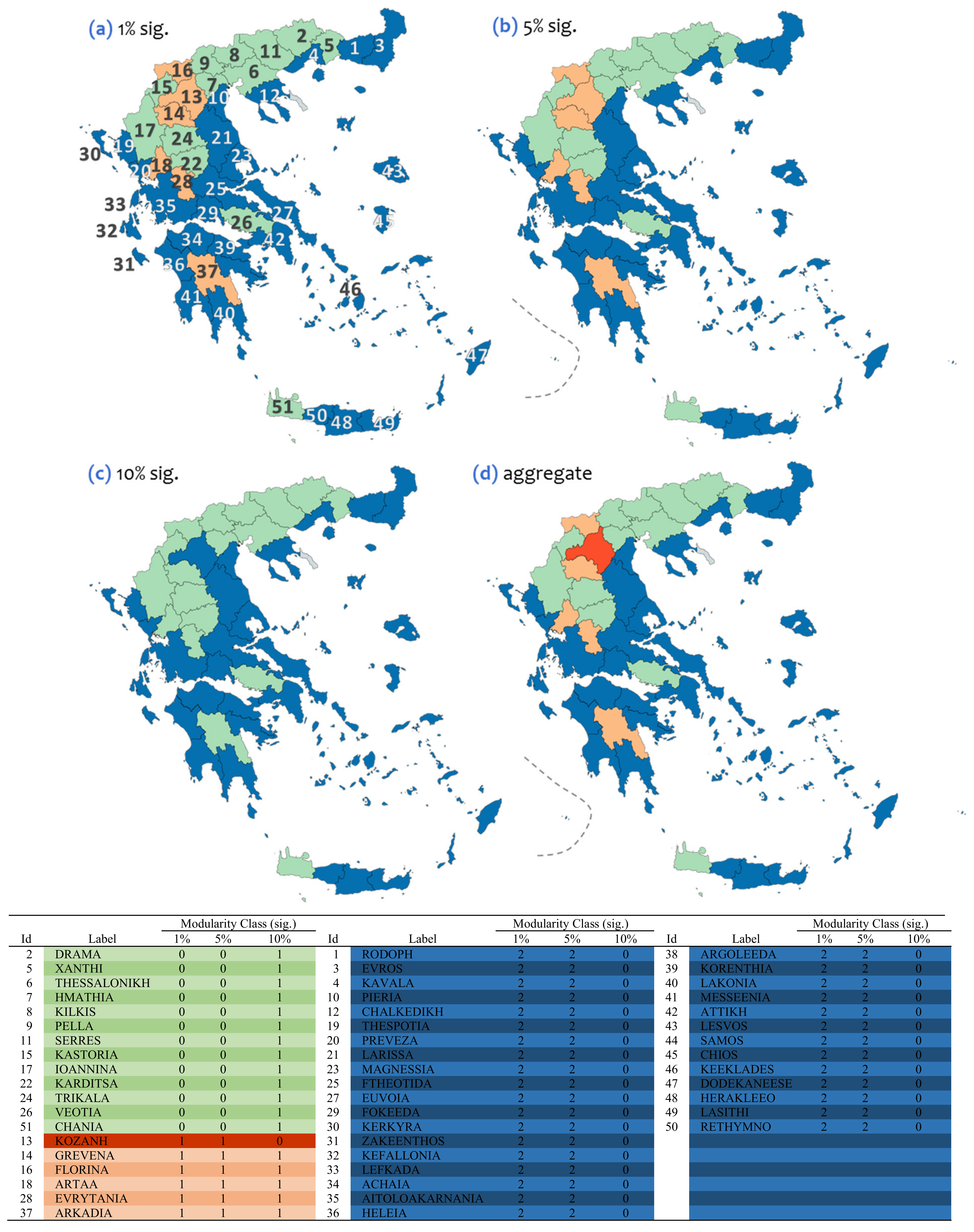
Figure 1. Conceptual diagram illustrating the methodology of the study.
Tourismhosp 02 00007 g001
Figure 2. Line-plots showing the time-series patterns of the available 51 seasonality-variables, which are shown in (left) metric and (right) semi-log scale. Each case (seasonality-variable) expresses a seasonality pattern of tourism overnight-stays (shown at the y-axis) that corresponds to one of the 51 prefectures in Greece. Seasonality-variables are of length 252, i.e., including 252 monthly records from January 1998 to December 2018. The available data were granted upon request by the Hellenic Statistical Authority [59] to be used under an exclusive license, for this study.
Tourismhosp 02 00007 g002
Figure 3. Het-maps showing the results of the correlation analysis applied to the available seasonality-variables (see Table A2 in the Appendix A), where case (a) shows correlations of sig. = 0.01, (b) of sig. = 0.05, and (c) of sig. = 0.10. At these correlation tables, only significant correlations are shown in color. (d) Distinguishable areas (A1, A2, and A3) of correlated variables in the correlation tables.
Tourismhosp 02 00007 g003
Figure 4. Maps showing the geographical location of the (a) A1, (b) A2, and (c) A3 areas, which are observed in the correlation analysis of Figure 3.
Tourismhosp 02 00007 g004
Figure 5. Geographical distribution and tabulation of the seasonality patterns that correspond to the Greek prefectures and are produced by the modularity classification for (a) 1%, (b) 5%, and (c) 10% levels of significance. Case (d) shows the aggregate patterns including the unique triplets of the (a), (b), and (c) modularity classes. Dashed lines illustrate shapes of spatial patterns.
Tourismhosp 02 00007 g005
Figure 6. Maps showing the geographical distribution of the available 51 seasonality patterns that are grouped (according to the modularity classification shown in Figure 5) to the modularity (triplet-) groups, as follows: (a) aggregate, including all 4 available groups, (b) (0,0,1), of an “S”-shaped spatial pattern, (c) (1,1,0), of a “dot”-shaped spatial pattern, (d) (1,1,1), of an “I”-shaped spatial pattern, and (e) (2,2,0), of an “O”-shaped spatial pattern.
Tourismhosp 02 00007 g006
Figure 7. Line plots with the time-series of the available 51 seasonality patterns that are grouped (according to the modularity classification shown in Figure 6) to the triplet-groups: (a) (0,0,1) of the “S”-shaped spatial pattern, (b) (1,1,0) of the “dot”-shaped spatial pattern, (c) (1,1,1) of the “I”-shaped spatial pattern, and (d) (2,2,0) of the “O”-shaped spatial pattern.
Tourismhosp 02 00007 g007
Figure 8. Error-bar plots representing 95% confidence intervals (95%CIs) for the mean values of (a) the Gini coefficient and (b) the RSI (Relative Seasonal Index).
Tourismhosp 02 00007 g008
Figure 9. Maps showing the geographical distribution of the Principal Components Analysis max-filtering groups (PCM) that are computed in the paper of [9], where (a) is the aggregate group, including all 5 available PCM groups, (b) is the PCM#1 group of an “O”-shaped spatial pattern, (c) is the PCM#2 group of a “U”-shaped spatial pattern, (d) is the PCM#3 group of an “I”-shaped spatial pattern, (e) is the PCM#4 group of a “dot”-shaped spatial pattern, and (f) is the PCM#5 group of a “dot”-shaped spatial pattern.
Tourismhosp 02 00007 g009
Figure 10. Maps showing the geographical distribution of the Principal Components Analysis min-filtering groups (PCm) that are computed in the paper of [9], where (a) is the aggregate group, including all 7 available PCm groups, (b) is the PCm#1 groups of a “dot”-shaped spatial pattern, (c) is the PCA#2 group of an “O”-shaped spatial pattern, (d) and (e) are the PCA#3 and PCA#4 groups of a “U”-shaped spatial patterns, (f) is the PCA#5 group of an “S”-shaped spatial pattern, and (g) and (h) are the PCA#6 and PCA#7 groups of an “I”-shaped spatial patterns.
Tourismhosp 02 00007 g010
Table 1. The semiology of the modularity groups (see Figure 5) resulted from the analysis.
Modularity Groups (Size)Socio-Economic and Geographical Semiology
MAX (a)MIN (b)
Group (0,0,1)
(13 prefectures)
Northern and eastern location; urbanization; specialization in winter tourism activities; environmental wealth.Area; seasonality; ports; camping; beaches.
Group (1,1,0)
(1 prefecture)
Northern and west location; rich geomorphological configuration; mainland geomorphology; rich rail and airport configuration; high secondary sector specialization; high mountainous activities.Coastal or island area; seasonality; poor road density and roads; low primary and tertiary sector specialization; low tourism profile; low environmental wealth, low cultural resources profile.
Group (1,1,1)
(5 prefectures)
Mainland geomorphology; urbanization; high tertiary sector specialization; high environmental wealth.Coastal or island area; poor geomorphological configuration; seasonality; poor ports and airports configuration; population and human capital; low income; low secondary sector specialization; low tourism profile; low beach environment; low cultural resources profile.
Group (2,2,0)
(32 prefectures)
Southern and eastern location; coastal or island area, high seasonality; rich road density and ports configuration; high urbanization; high primary and tertiary sector specialization; high tourism profile; high environmental quality; high capacity of cultural resources.Poor geomorphological configuration; poor rail configuration; low secondary sector specialization; low mountainous activities.
(a) as defined by the max values of Table A4 (see Appendix A). (b) as defined by the min values of Table A4 (see Appendix A).
Table 2. Multi-block comparative table showing the intersection results P C # i M O D # j (window: Intersection Frequencies) between i-th PCA and j-th modularity groups, with j = (2,2,0), (0,0,1), (1,1,1), or (1,1,0), their percentage (%) relevance to the PCA/MOD groups (window: Relevance to PCA/MOD Groups), and a metric test (window: Differences in Relevance) implying which (PCA/MOD) group is dominant for each intersection.
Modularity Group
Group Size
321351321351321351321351
Group Label
(2,2,0)(0,0,1)(1,1,1)(1,1,0)(2,2,0)(0,0,1)(1,1,1)(1,1,0)(2,2,0)(0,0,1)(1,1,1)(1,1,0)(2,2,0)(0,0,1)(1,1,1)(1,1,0)
Common Cases Between MOD and PCA Groups (intersection)
Group SizeGroup Label◂Relevance to PCA GroupsIntersection Frequencies▴Relevance to MOD GroupsDifferences in Relevance (MOD-PCA)
PCA Group#1 (max filtering)38PCM#184.2%13.2%2.6% 3251 100%38.5%20.0% 15.8%25.3%17.4%
7PCM#2 100% 7 53.8% −46.2%
4PCM#3 100% 4 80.0% −20.0%
1PCM#4 100% 1 100%
1PCM#5 100% 1 7.7% −92.3%
#2 (min filtering)1PCM#1 100% 1 7.7% −92.3%
7PCM#285.7% 14.3% 6 1 18.8% 20.0% −67.0% 5.7%
13PCM#369.2%30.8% 94 28.1%30.8% −41.1%
14PCM#47.1%14.3%14.3% 122 3.1%15.4%40.0% −4.0%1.1%25.7%
8PCM#550.0%37.5% 12.5%43 112.5%23.1% 100%−37.5%−14.4% 87.5%
5PCM#620.0%40.0%40.0% 122 3.1%15.4%40.0% −16.9%−24.6%
3PCM#766.7%33.3% 21 6.3%7.7% −60.4%−25.6%
Lagend0%0–20%20–40%40–60%60–80%≥80%%PCA < 0MOD > 0
Publisher’s Note: MDPI stays neutral with regard to jurisdictional claims in published maps and institutional affiliations.

