Aggregated Gaze Data Visualization Using Contiguous Irregular Cartograms


Department of Surveying and Geoinformatics Engineering, School of Engineering, University of West Attica, 28 Agiou Spyridonos Str., 12243 Egaleo, Greece
Digital 2021, 1(3), 130-144; https://0-doi-org.brum.beds.ac.uk/10.3390/digital1030010
Submission received: 7 May 2021
/
Revised: 28 June 2021
/
Accepted: 29 June 2021
/
Published: 30 June 2021
Abstract
:Gaze data visualization constitutes one of the most critical processes during eye-tracking analysis. Considering that modern devices are able to collect gaze data in extremely high frequencies, the visualization of the collected aggregated gaze data is quite challenging. In the present study, contiguous irregular cartograms are used as a method to visualize eye-tracking data captured by several observers during the observation of a visual stimulus. The followed approach utilizes a statistical grayscale heatmap as the main input and, hence, it is independent of the total number of the recorded raw gaze data. Indicative examples, based on different parameters/conditions and heatmap grid sizes, are provided in order to highlight their influence on the final image of the produced visualization. Moreover, two analysis metrics, referred to as center displacement (CD) and area change (AC), are proposed and implemented in order to quantify the geometric changes (in both position and area) that accompany the topological transformation of the initial heatmap grids, as well as to deliver specific guidelines for the execution of the used algorithm. The provided visualizations are generated using open-source software in a geographic information system.
1. Introduction
The process of recording and analyzing eye-tracking data constitutes one of the most popular techniques for the examination of both perceptual and cognitive aspects related to human visual behavior. Gaze data could serve as a quantitative and objective input towards visual attention modeling and prediction while, at the same time, they can be utilized in order to indicate the user reaction during the manipulation of different types of devices, including both typical computers and mobile devices (e.g., smartphones). Hence, the importance of eye-tracking methods is direct and clear in several studies and applied domains related (but not limited) to behavioral analysis, artificial intelligence and human–computer interaction (HCI). Moreover, several recent studies have presented the wide range and influence of eye-tracking applications in different disciplines, such as medical education [1], diagnostic interpretation [2], multimedia learning [3], software engineering [4], computer programming [5], aviation [6], mathematics education [7], cartography [8], behavioral economics and finance [9], marketing [10], and tourism [11]. The broad diversity of the aforementioned domains confirms both the popularity and the effectiveness of the method.
An eye-tracking data protocol consists of the spatiotemporal coordinates collected during the observation of a visual stimulus in two (2D) or three (3D) dimensional space. More specifically, eye movements could be recorded using a typical 2D monitor attached to a digital device (i.e., computer, smartphone or tablet display, television, or any image projected in 2D space using a projector device), in 3D natural space (environment), or in a 3D virtual environment. In practice, eye movement examination mainly analyzes the recording gaze data in both fundamental (i.e., fixation and saccades) and derived metrics [12] by implementing event detection algorithms (see, e.g., the work described by Ooms and Krassanakis [13] for further details). Additionally, the implementation of several visualization methods could substantially support eye movement analysis revealing critical patterns indicated by the computed fixations, saccades, and scanpaths [14]. Over the last years, several methods for gaze data visualization have been proposed (see, e.g., [15]), including both simple (e.g., scanpath plots) or more sophisticated techniques that could highlight the visual behavior of several observers. Among the big challenges in gaze data visualization techniques, the development of 2D (static) visualizations for the depiction of spatiotemporal data (see, e.g., the method presented in [16]) as well as for the visual representation of the cumulative (based on different observers) visual behavior is of major importance. A taxonomy followed by Blascheck et al. [17] groups eye-tracking visualization methods into two main categories: the point-based and the area of interest (AOI)-based techniques. Considering the existing analysis approaches followed (in different research and practical domains) in eye-tracking research, this discrimination can be considered quite representative and helpful. Additionally, the development and the evaluation of new approaches for the visualization of gaze data could substantially contribute to indicate hidden patterns revealed by eye-tracking recordings. Hence, this statement motivates the performance of related research towards this direction. Except for the techniques that are mainly dedicated to the visualization of the visual scanning behavior of each individual, techniques that are able to support the visualization of aggregated gaze data and therefore to indicate the overall visual behavior considering inputs by multiple observers, could have a significant influence in both the interpretation and modeling of visual perception and attention processes. The significance of visualization methods in eye-tracking analyses and usability studies can also be demonstrated by the fact that many software, including standalone packages (e.g., OGAMA [18]) or toolboxes (e.g., EyeMMV toolbox [19]) working in local or in web environment (see e.g., the tools described in previous studies [20,21]) implement several methods that are utilized in conjunction with the typical metric-based analyses.
The present study aims to describe the application of the method of contiguous irregular cartograms as a technique for aggregated gazed data visualization. An existing sub-dataset of gaze data is used in order to provide representative examples, while the implementation of the method is completed utilizing open-source tools in a geographic information system. Since the used method is based on the topological transformation of a typical grayscale heatmap, two new metrics are proposed and computed in order to reveal the overall distortion of the used heatmap grids.
The sections below describe the state-of-the-art in the examined field and describe the implementation of the performed study towards the production of the proposed visualizations. The provided outcomes are based on the computation of the proposed metrics (CD and AC) and aim to deliver specific guidelines for the execution of the used algorithm. Finally, the provided approach is discussed and summarized, providing, at the same time, possible extensions of the current work.
2. Related Work
2.1. Aggregated Gaze Data Visualization
The visualization of aggregated gaze data constitutes an essential part that accompanies the data analysis process in eye-tracking studies. Aggregated gaze data visualization methods are used in order to highlight the spatiotemporal allocation of visual attention during the observation of a visual stimulus. The utilization of such techniques mainly aids the qualitative examination of the tested visual stimuli, providing, at the same time, a representative overview of the scanning behavior. Heatmap visualization is the most popular technique for aggregated gaze data presentation. This method is able to directly depict eye-tracking data distribution [22]. Bojko [23] summarized different approaches that could be accomplished towards the implementation of heatmap visualizations, also pointing out best practices that must be followed for their construction and interpretation. The heatmap visualization method could be applied in both static and dynamic stimuli as a post-experimental or real-time (see, e.g., the work presented in [24]) procedure; however, several other approaches have been recently proposed in the literature.
Kurzhals et al. [25] presented the gaze stripes method, which is suitable for both static and dynamic (i.e., animations or simple video) visual stimuli. The method uses the sequence of gaze point images along a horizontal timeline in order to reveal and compare patterns among different scan paths [25]. The power of this method is that it does not require the delineation of specific AOIs along the visual stimuli while at the same time the examination of the generated patterns is based on the simple alignment of multiple gaze stripes produced by different observers. Furthermore, Burch et al. [26] introduced, as an addition to heatmap and gaze stripes visualization techniques, the concept of attention cloud as a method to depict the parts of a visual stimulus that are observed for the longest amount of time. More specifically, each cloud corresponds to a cropped circular image with an area proportional to observers’ fixation durations.
The utilization of multiple AOIs analyses could enhance the function of existing approaches that aim to visualize the overall patterns produced during the observation of visual stimuli by delivering practical approaches to also perform statistical analyses (see, e.g., the work presented by Kurzhals and Weiskopf [27]). The visualization of the aggregated gaze behavior could be implemented by the application of AOI-based techniques. For example, the concept of “one glance” parallel scan path comparison proposed by Raschke et al. [28] is based on specific AOIs, while Burch et al. [29] implemented AOI-based hierarchical flows as an alternative approach to exploring eye movements. Additionally, a recent technique called Sankeye was presented by Burch and Timmermans [30], uses flow maps (Sankey diagrams), and aims to visualize transitions among AOIs by encoding transactions’ frequencies into left-to-right directions characterized by different flows’ thicknesses.
2.2. Statistical Grayscale Heatmaps
Statistical grayscale heatmaps constitute quantitative products developed considering the spatial distribution of point data. In eye-tracking research, these points could be referred either to the raw gaze data or to the (analyzed) points resulted after the computation of the fixation points’ centers based on the implementation of a fixation detection algorithm. In both cases, the input points have spatiotemporal characteristics (for the case of gaze data, the temporal dimension corresponds to the passing time connected to the recording process, while for the case of fixation points, it corresponds to the extracted fixations’ durations). Although both approaches could be considered appropriate for heatmap generation [19], in the case of the statistical grayscale heatmap, the optimal quality of the final product can be achieved using the spatial distribution of the raw gaze point data since uncertainties influenced by the implemented fixation detection algorithm could be avoided; however, the uncertainties (noise) existed due to the used eye-tracking equipment, missing data, and blinks.
The generation of a statistical grayscale heatmap is based on the application of a typical Gaussian filter with two basic parameters, including kernel size and standard deviation (sigma). Furthermore, this filtering process is applied for each pixel of the visual stimulus considering the aforementioned parameters based on the foveal range, which corresponds to 1° of the visual angle. After the implementation of the Gaussian filtering, the produced values are normalized by dividing all pixel values by the maximum produced value. The result of this process maps all the values to the range [0,1]. In the next step, all values are multiplied with the constant 255 (28 intensities) in order to produce the grayscale statistical heatmap. In the end, this statistical product is able to indicate the possibility of having a gaze point in each pixel, highlighting at the same time the salient locations within the visual stimulus. Hence, it can be used for both qualitative and quantitative evaluation. However, based on this normalization approach, the maximum value may express different situations (e.g., durations) for different visual stimuli.
It is worth mentioning that several existing tools (e.g., [19,31]) support the generation of statistical grayscale heatmaps while such products constitute the main components of the publicly available eye-tracking datasets (e.g., [32,33]). Moreover, taking into account that the nature of computer mouse movements data is identical to eye movements, grayscale statistical heatmaps could also be produced based on data recorded with mouse tracking techniques (see, e.g., the recent work presented by Krassanakis and Kesidis [34]).
2.3. Contiguous Irregular Cartograms
Cartograms constitute thematic map visualizations that are mainly used in order to represent phenomena distributed in space (e.g., population mapping). In recent years, this type of visualization has become popular, having several applications in different domains [35], and especially fields related to cartography [36,37] and spatial analysis [38], providing fruitful information related to socio-economic conditions (see, e.g., the work presented in [39]). The implementation of a cartogram is based on the proportional distortion of a feature distance or area according to the value of the data that have to be visualized [40]. Cartograms can be classified into several categories based on different criteria. For example, Field [37] classified cartograms into four main categories, including non-contiguous, contiguous, graphical, and gridded cartograms. A more detailed classification based on different criteria, including mathematical basis, transformed object, and method, graphic continuity and presentation, grid transformation and the main distortion of points location is recently provided by Markowska [40]. Three main types can be distinguished depending on the shape of mapping units: proportional symbol cartograms, continuous (contiguous) regular cartograms, and continuous (contiguous) irregular cartograms [41]. According to the definitions given by Markowska [40,41], contiguous irregular cartograms referred to the method “where the shapes of areal units on the map resemble the actual shapes of the mapped units but unit boundaries are not straight lines” ([41], p. 19), while the “base units correspond to the shape of statistical units, their borders are not geometrized, the shape of units depends on the distortion algorithm applied” ([40], p. 54).
Several algorithms (see, e.g., the algorithms recently described by Gastner et al. [42] and by Sun [43]) have been developed in order to support the implementation of cartogram visualization (further details [37,40,41,44], as well as comparisons [41], are available in previous studies). Moreover, different tools suitable for cartogram production are also available either as standalone packages (e.g., ScapeToad (http://scapetoad.choros.place/, accessed on 7 May 2021) software) or as tools working as plugins or addons in geographic information software (GIS) tools. Furthermore, specific types of cartograms (circular cartograms—also known as Dorling cartograms) are implemented in GeoDa (https://geodacenter.github.io/, accessed on 7 May 2021), which is a complete open-source software for spatial analysis. As an example for indicating the availability of the existing tools, an in depth evaluation oriented to area cartograms was presented by Markowska [41] for the interested reader.
3. Materials and Methods
3.1. Gaze Data
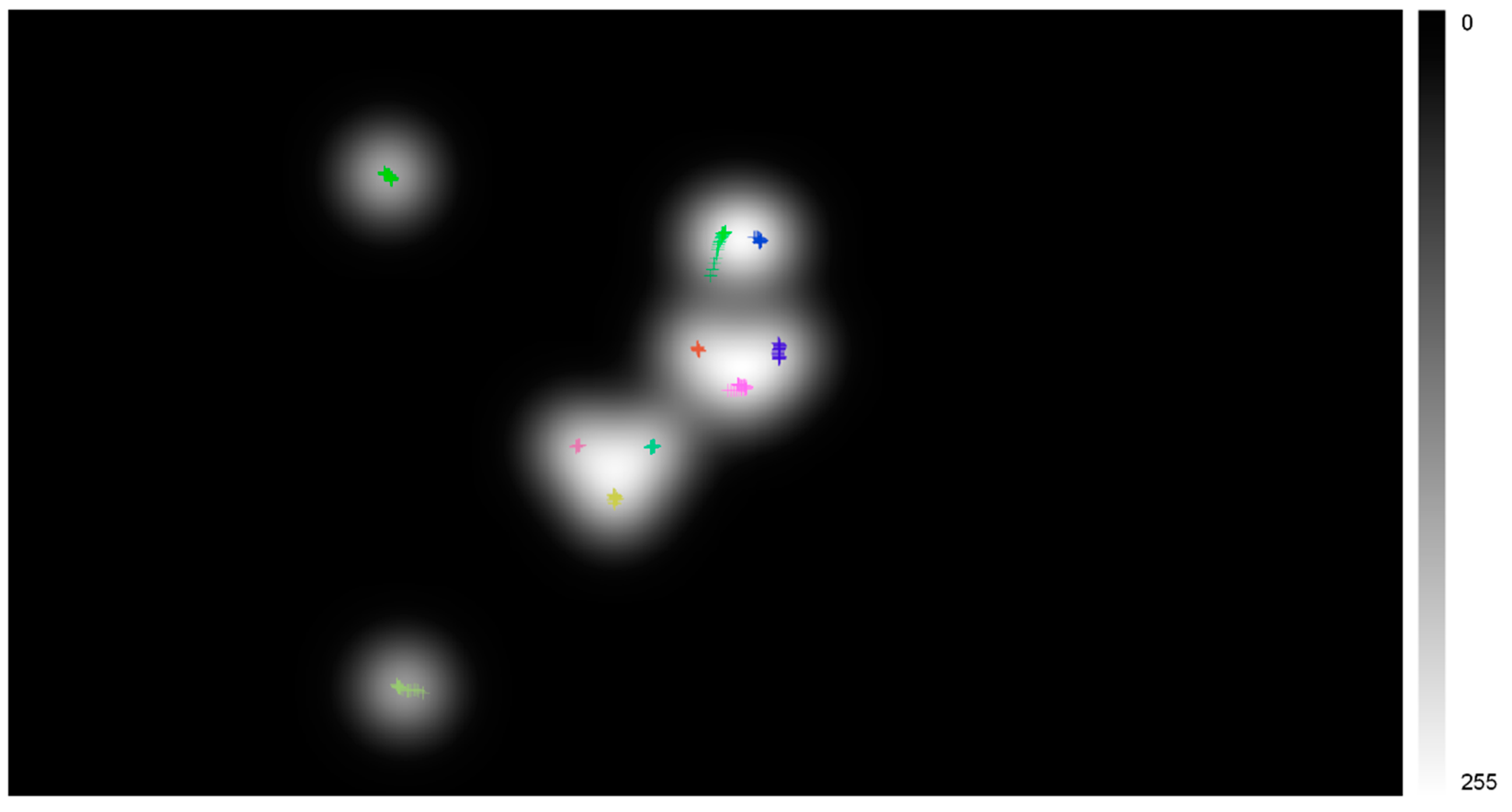
A statistical grayscale heatmap distributed with EyeTrackUAV [32] eye-tracking dataset was used for the performance of the present study. The EyeTrackUAV dataset has been generated [32] based on the gaze data recorded by fourteen participants during the observation of UAV videos under free-viewing conditions (without any task required to be executed). The sampling frequency used for eye-tracking recording in this dataset was equal to 1000 Hz, while the used videos of EyeTrackUAV are a part of the videos available from the UAV123 database [45]. For the purposes of the present study, the first statistical grayscale heatmap of the subset “building5” of the EyeTrackUAV dataset was utilized. The native resolution of the grayscale heatmap was equal to 1280 × 720 px (720p resolution). This grayscale statistical heatmap was generated in the EyeMMV toolbox [19] considering a grid size (gs) equal to 1 px, a standard deviation (sigma) equal to 32 px (0.5° of the visual angle), and a kernel size (ks) that corresponds to the value of 6*sigma [32]. In Figure 1, the statistical grayscale heatmap is presented alongside the raw gaze data collected by the different observers.
All values of the used statistical grayscale heatmap are normalized to the range between 0 and 255 (28 different intensities). In order to highlight the dispersion of the normalized values of the statistical grayscale heatmap values, some basic statistics were calculated and presented in Table 1.
3.2. Cartograms Implementation
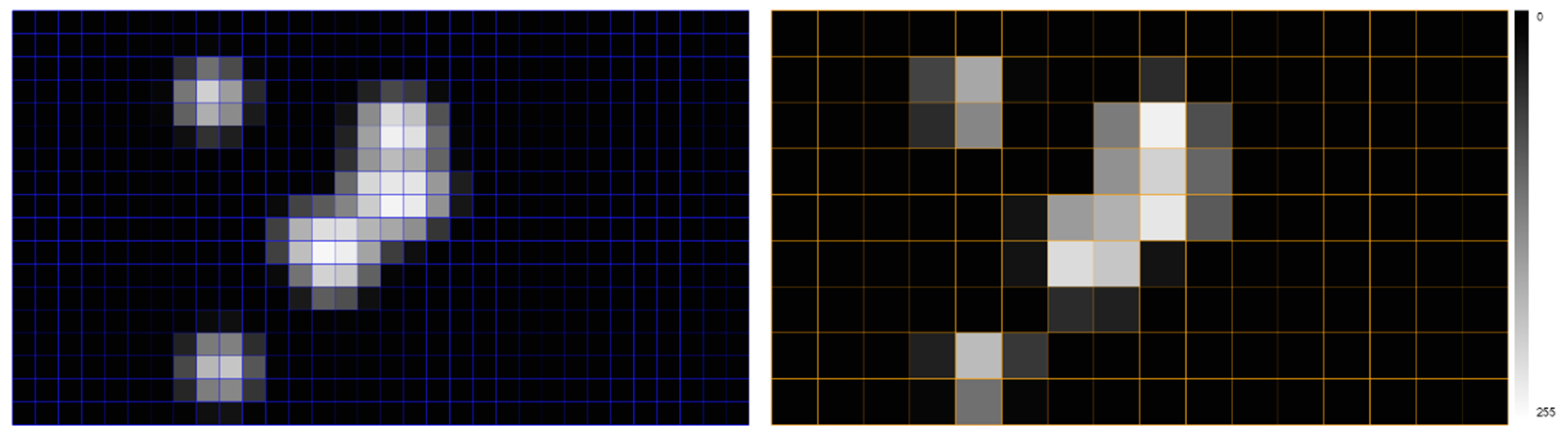
Since the aim of the present study is to provide critical indications about the process of aggregated eye-tracking data visualization, the initial information involved in the statistical grayscale heatmap was downscaled. In this way, the overall execution time was substantially decreased. In more detail, the initial resolution of the statistical grayscale statistical heatmap was decreased considering pixel sizes 5, 10, 20, 40, and 80 times larger than the corresponding size of the raw product, which resulted in grid resolutions equal to 256 × 144, 128 × 72, 64 × 36, 32 × 18, and 16 × 9 accordingly. The production of these heatmaps was made in QGIS software (https://www.qgis.org/, accessed on 7 May 2021) which is a free and open-source geographic information system (GIS), while it is a result of the nearest neighbor interpolation method. After several running tests, two heatmaps were used for the performance of the present study: ‘heatmap40’ with a grid resolution equal to 32 × 18 units (pixel size is 40 times smaller than the initial) and ‘heatmap80’ with a grid resolution equal to 16 × 9 units (pixel size is 80 times smaller than the initial). Therefore, the area of each cell is equal to 1600 px2 (40 × 40 px) and 6400 px2 (80 × 80 px) and corresponds to approximately 0.17% and 0.69% of the grayscale statistical heatmap for ‘heatmap40’ and ‘heatmap80’, respectively. Selecting the specific grid resolutions, the produced results are interpretable since discrete differences (among different grid cells) are highlighted and can be easily distinguished. Although the grid size is different in the two heatmaps, their spatial extent, as well as their coordinate system, remains the same. More specifically, both heatmaps are expressed in the pixel coordinate system and borrow their extent from the initial resolution of the raw product (horizontally: 1280 px and vertically 720 px). Hence, this approach supports the direct comparison between the two cases (as well as among any other case of heatmap with different cell sizes). Moreover, the produced heatmaps have all the advantages of the gridded cartograms [39,46] while, concurrently, they consider the whole region of the examined visual scene. Both produced heatmaps are depicted in Figure 2.
The generation of the irregular contiguous cartograms was based on the execution of the ‘cartogram3′ (https://github.com/austromorph/cartogram3, accessed on 7 May 2021) software tool. This tool works as a plugin that is embedded in QGIS software. The plugin generates anamorphic maps using polygon data. Therefore, both heatmaps were transformed into vector data using the typical raster to vector transformation implemented in the QGIS software. The ‘cartogram3’ QGIS plugin was developed using Python v.3 and PyQt5 and implemented the algorithm proposed by Dougenik et al. [47]. The plugin considers two main input parameters—conditions for its execution, including the maximum number of iterations as well as the maximum average error achieved, expressed as a number and as a percentage accordingly. Once one of the conditions is attained, the computed calculation stops and the corresponding cartogram is produced. This means that the produced result does not always follow the optimal rule according to which the transformed polygons must be proportional to the qualitative data used for the generation of the cartogram. Therefore, different combinations of parameters could have a direct influence on both the effectiveness and the efficiency of the implemented algorithm. The effectiveness of the algorithm is connected to its ability to transform proportionally to the input data of each polygon, and to the efficiency of the overall processing time and execution speed.
In order to highlight the influence of the selected parameters, the produced cartograms were generated considering four different combinations of parameters/conditions. More specifically, for all combinations, the maximum average error was selected to be equal to 1%, and the cartograms produced after 50, 100, 200, and 400 iterations after considering both heatmaps in polygon vector format—the specific value of maximum average error selected after several trials. As also mentioned above, since the implemented algorithm stops once one of the conditions achieved and considering that the selected value was quite difficult to be met with the specific dataset, in practice, the parameter-condition of the total number of iterations seems to play the most significant role in the procedure, and hence to the final visualization.
3.3. Quantitative Evaluation Metrics
The selected combinations reported in Section 3.2, resulted in the generation of 8 different visualizations, including four cartograms for each heatmap. The produced visualizations consist of anamorphic maps, which retain the basic topological property of boundaries sharing among the grids’ cells. However, both the positions and the shape of the corresponding cells changed after their transformation. In order to evaluate the magnitude of these deformations, two main metrics are proposed and implemented in the present study:
- CD metric: This metric refers to the cell’s center displacement after the implementation of the cartogram algorithm. For each corresponding cell, the CD can be computed as the Euclidean distance between two points: the geometric center of the cell before the transformation (first point) and the geometric center of the same cell after the transformation. Hence, the computation of CD metric is in distance units (e.g., in pixels). CD values are greater or equal to zero. A CD value equal to zero indicates that the geometric center of the cells remains constant after the topological transformation.
- AC metric: This metric refers to the area change between two corresponding cells (before and after the implementation of the cartogram algorithm). Therefore, this metric is computed using the formula (A2 − A1)/A1, where A1 and A2 correspond to the areas before and after the transformation accordingly. The AC can also be expressed as a percentage (%) if this ratio will be multiplied by the value of 100%. However, considering that bigger changes may have resulted in bigger AC values (greater than 100%) it is not always quite representative to express the metric as a percentage. Positive AC values indicate that the cell’s area increased after the transformation and negative AC values indicate that the area decreased. Zero values of AC indicate the absence of any area change.
In practice, considering that a regular grid serves as the starting point (before any deformation), the aforementioned metrics could be used as quantitative indicators that are able to highlight the overall transformation of the grid. Hence, CD and AC values are meaningful only in the framework of the proposed (“grid-based”) approach. Therefore, both metrics cannot be implemented in the case that irregular (without specific shape) polygons are utilized as the main input (as it happens with typical geographic data) to the performed algorithm for cartogram generation. For the purposes of the present study, the extraction of the geometric centers’ coordinates as well as the computation of cells’ areas was based on typical functions and tools provided by QGIS software and used for vector data manipulation.
4. Results
The results of the present study involve both the qualitative visualizations of the aggregated gaze data referred to different observers as well as the quantitative evaluation of the produced outcomes based on the computation of both CD and AC metrics.
4.1. Aggregated Gaze Data Visualizations
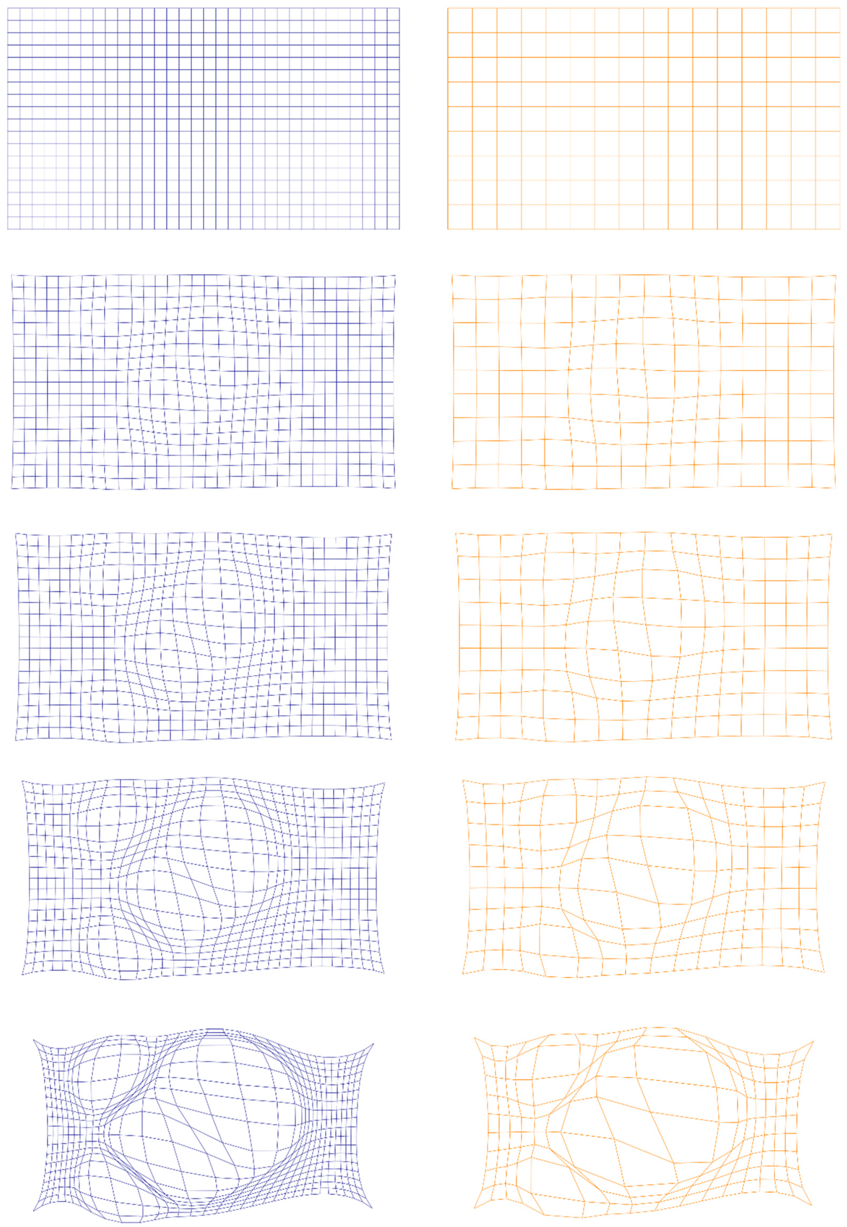
The aggregated gaze data were visualized as continuous irregular cartograms considering the different combinations of selected parameters/conditions reported in the methodology described above. Both the initial conditions (heatmap grids) and the transformed visualizations (cartograms) for each heatmap and for all selected parameters are depicted in Figure 3. As is highlighted, the number of iterations directly affects the overall transformation of the initial grids for both heatmaps (Figure 3). Considering that the initial conditions are characterized by uniform grids, the magnitude of changes in cells’ size specifies the allocation of visual attention based on the collected gaze data.
4.2. CD and AC Metrics Visualizations
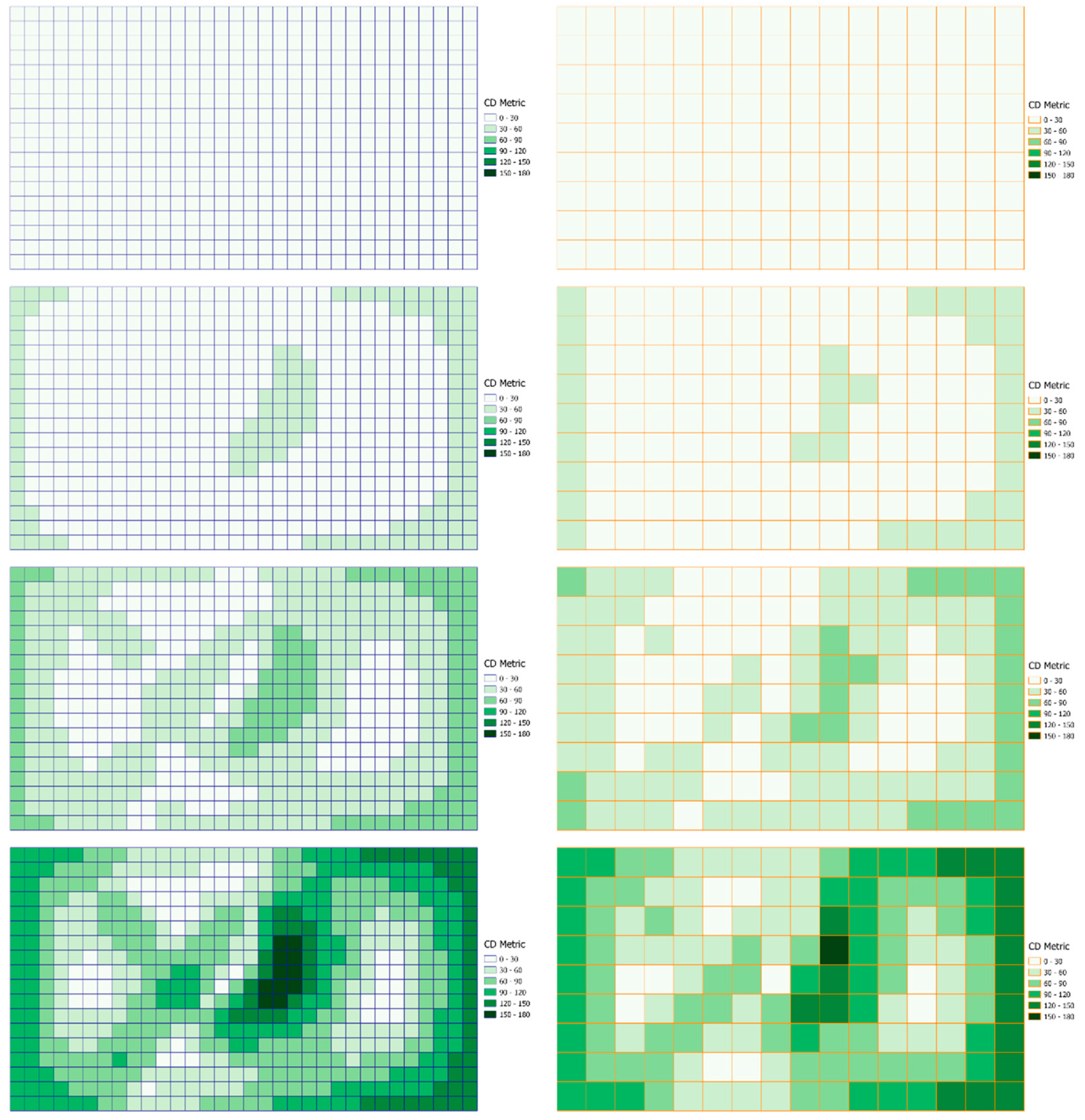
Both CD and AC metrics were calculated for all produced cartograms in order to quantify the magnitude of the grid’s deformation. The produced results are visualized after a uniform classification of the produced values for both CD and AC metrics. More specifically, CD and AC values were classified considering an equal interval classification using six classes and the range of the computed quantities for all cases in order to deliver comparable results. Taking into account the minimum and maximum values, for the case of CD metric, the selected groups involve the classes [0–30), [30–60), [60–90), [90–120), [120–150), and [150–180), expressed in pixels. The results of the CD metric are depicted in Figure 4.
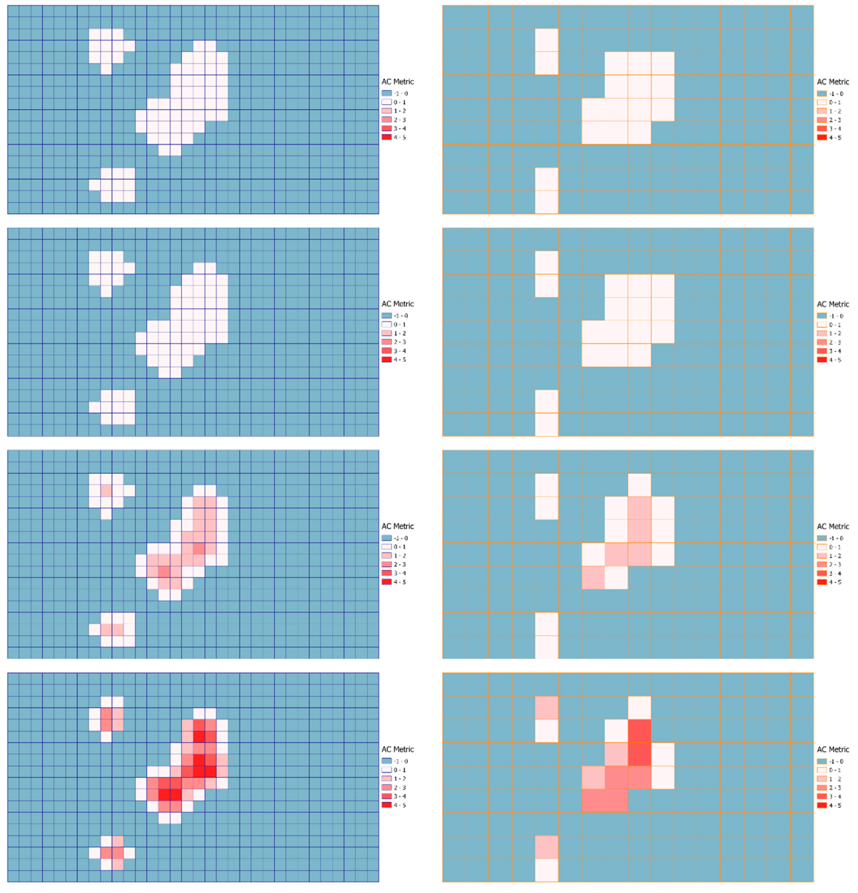
In Figure 5, the results of the AC metric are visualized after the classification of the produced values into six classes considering the range of all values. The used groups include the classes [(−1)–0), [0–1), [1–2), [2–3), [3–4), and [4,5).
4.3. CD and AC Metrics Analysis
Except for the visualization of the reported values that characterize each metric for all examined cases, representative statistics were also computed in order to better describe the deformations accompanying the produced cartograms. The result for both cases of ‘heatmap40’ and ‘heatmap80’ are presented in Table 2.
Moreover, considering as a threshold the size of the grid cell, the total number of cases that resulted in CD values higher than this threshold were calculated as a percentage for both heatmap cases. For the case of the AC metric, the corresponding percentages of negative and positive values were also calculated. Additionally, in order to better highlight the distribution of the AC values, the percentages that correspond to absolute AC values higher than 20% (and hence to positive or negative changes higher than 20%) were also calculated. The relative results of the aforementioned computations are presented in Table 3.
Considering the initial total area of both grids (same for both heatmaps and equal to 1280 × 720 = 921,600 px2), the overall area change of the produced cartograms was also computed in order to serve as an indicator of the total deformation of the whole visualization area. The results for all cases (different number of iterations) are presented in Table 4.
5. Discussion and Conclusions
The implementation of the cartogram algorithm resulted in the visualization of aggregated gaze data recorded by different participants. More specifically, different combinations of parameters/conditions were used in order to highlight the overall behavior of the performed algorithm towards the production of the contiguous irregular cartograms. Considering that the maximum average error was selected to be constant in all combinations, the parameters of the different number of iterations were the main condition that affected the final shape of the produced cartograms. Hence, testing different numbers of iterations, the produced outcomes indicate the level of transformation applied in the initial grid. At this point, it is far too important to mention that the number of iterations in the performed algorithm could serve as a stopping criterion in order to ensure that the execution of the process is not endless when the produced distortions have become quite severe to prevent topological errors. As also explained in Section 3.2, in this way, the produced polygon (i.e., grid cell) does not always follow the optimal rule of the proportional to qualitative data transformation of each cell. However, during the execution of the used algorithm, there is a specific point that additional iterations no longer change the final grid. The provided method serves as an alternative to other typical methods that are used in order to visualize the allocation of the gaze behavior during the observation of a visual stimulus. Some approaches have also been followed in other studies that propose either the generation of typical heatmaps that referred to the whole area of a stimulus or visualizations that referred to visual stimuli with specific characteristics (e.g., line stimuli [48]). However, the presented approach was based on the application of a specific technique, mainly applied in geographic data.
The produced cartograms are able to indicate the areas of the stimulus where visual attention is devoted. In the framework of the present examination, two different heatmaps were produced and further examined. In both cases, cartograms were able to point out the most salient regions of the visual scene revealed by the grid cells that were accompanying both positional and area distortions. After a qualitative examination of both grids, the size of cells seems to influence the final representation of the produced visualization (Figure 3). As a matter of fact, using a smaller sized grid cell leads to a more accurate representation. This is also the case when a typical heatmap is used; however, in order to quantify the overall deformation of the used grids, two specific metrics were proposed and implemented. Both metrics consider geometric characteristics of the fundamental elements (cells) of the produced grids. Even the visualizations of the CD and AC values per cell (Figure 4 and Figure 5) are able to reveal the generated pattern of visual attention allocation and could be used as a method for heatmap generation; an alternative to these reported by Bojko [23].
The results produced by the analysis CD and AC values (Table 2 and Table 3) show that the selected number of iterations plays a significant role in the production of the final visualization. The overall spatial transformation of the heatmap grid is directly influenced by the total number of iterations. Taking into account that the delivered cartograms are contiguous and therefore the topological connections among the cells must remain constant, the higher number of iterations also resulted in the minimization of the cell sizes where no gaze data were recorded. At the same time, the percentages reported in Table 3 (AC metric) proves that the overall cell areas decreased in order to highlight the regions where gaze points were recorded. This outcome is also compatible with the results referred to the overall area of the produced visualization reported in Table 4 for all the cases of the selected number of iterations.
The results provided in the present study could give some first guidelines towards the adaptation of geographical-inspired methods in eye-tracking visualization. The utilization of contiguous irregular cartograms towards the visualization of overall (aggregated) visual behavior contributes to the state-of-the-art of the discussed field. The study shows how the proposed visualization could be implemented based on the execution of open-source software tools. However, the development of dedicated software tools oriented to gaze data analysis is an obvious extension of the presented work. Additionally, several other methods for cartogram generation could be tested using open-source software. For example, the approach of the famous “Dorling” diagrams is supported by the open-source tool GeoDa. The suggested approach is similar to the concept of EyeClouds recently described by Burch [26]. Finally, since a typical grayscale heatmap was used as the main input in order to generate the final cartograms, the proposed method could also be implemented in other types of behavior data, such as records collected by computerized mouse movements [34]. At the same time, the main advantage of using this specific input is the fact that its nature is independent of the total amount of the recorded gaze (or mouse) data. Therefore, the provided approach is fully compatible with any recording frequency applied by the used eye-tracking equipment.
Funding
This research received no external funding.
Institutional Review Board Statement
Not applicable.
Informed Consent Statement
Not applicable.
Data Availability Statement
Not applicable.
Conflicts of Interest
The author declares no conflict of interest.
References
- Ashraf, H.; Sodergren, M.H.; Merali, N.; Mylonas, G.; Singh, H.; Darzi, A. Eye-tracking technology in medical education: A systematic review. Med. Teach. 2018, 40, 62–69. [Google Scholar] [CrossRef] [PubMed]
- Brunyé, T.T.; Drew, T.; Weaver, D.L.; Elmore, J.G. A review of eye tracking for understanding and improving diagnostic interpretation. Cogn. Res. Princ. Implic. 2019, 4, 7. [Google Scholar] [CrossRef]
- Alemdag, E.; Cagiltay, K. A systematic review of eye tracking research on multimedia learning. Comput. Educ. 2018, 125, 413–428. [Google Scholar] [CrossRef]
- Sharafi, Z.; Soh, Z.; Guéhéneuc, Y.-G. A systematic literature review on the usage of eye-tracking in software engineering. Inf. Softw. Technol. 2015, 67, 79–107. [Google Scholar] [CrossRef]
- Obaidellah, U.; Al Haek, M.; Cheng, P.C.-H. A survey on the usage of eye-tracking in computer programming. ACM Comput. Surv. 2018, 51. [Google Scholar] [CrossRef]
- Peißl, S.; Wickens, C.D.; Baruah, R. Eye-tracking measures in aviation: A selective literature review. Int. J. Aerosp. Psychol. 2018, 28, 98–112. [Google Scholar] [CrossRef]
- Strohmaier, A.R.; MacKay, K.J.; Obersteiner, A.; Reiss, K.M. Eye-tracking methodology in mathematics education research: A systematic literature review. Educ. Stud. Math. 2020, 104, 147–200. [Google Scholar] [CrossRef]
- Krassanakis, V.; Cybulski, P. A review on eye movement analysis in map reading process: The status of the last decade. Geod. Cartogr. 2019, 68, 191–209. [Google Scholar] [CrossRef]
- Sickmann, J.; Le, H.B.N. Eye-tracking in behavioural economics and finance—A literature review. Discuss. Pap. Behav. Sci. Econ. 2016, 2016, 1–40. [Google Scholar]
- Wedel, M. Attention research in marketing: A review of eye-tracking studies. In The Handbook of Attention; Boston Review: Cambridge, MA, USA, 2015; pp. 569–588. ISBN1 978-0-262-02969-8. (Hardcover); ISBN2 978-0-262-33187-6. (Digital (undefined format)). [Google Scholar]
- Scott, N.; Zhang, R.; Le, D.; Moyle, B. A review of eye-tracking research in tourism. Curr. Issues Tour. 2019, 22, 1244–1261. [Google Scholar] [CrossRef]
- Goldberg, J.H.; Helfman, J.I. Comparing information graphics: A critical look at eye tracking. In Proceedings of the 3rd BELIV’10 Workshop: BEyond Time and Errors: Novel EvaLuation Methods for Information Visualization, Atlanta, GA, USA, 10–11 April 2010; Association for Computing Machinery: New York, NY, USA, 2010; pp. 71–78. [Google Scholar]
- Ooms, K.; Krassanakis, V. Measuring the spatial noise of a low-cost eye tracker to enhance fixation detection. J. Imaging 2018, 4, 96. [Google Scholar] [CrossRef] [Green Version]
- Blascheck, T.; Kurzhals, K.; Raschke, M.; Burch, M.; Weiskopf, D.; Ertl, T. State-of-the-art of visualization for eye tracking data. In Proceedings of the EuroVis-STARs; Borgo, R., Maciejewski, R., Viola, I., Eds.; The Eurographics Association: Geneve, Switzerland, 2014. [Google Scholar]
- Burch, M.; Chuang, L.; Fisher, B.; Schmidt, A.; Weiskopf, D. Eye Tracking and Visualization: Foundations, Techniques, and Applications. ETVIS 2015, 1st ed.; Springer: Berlin/Heidelberg, Germany, 2017; ISBN 331947023X. [Google Scholar]
- Räihä, K.-J.; Aula, A.; Majaranta, P.; Rantala, H.; Koivunen, K. Static visualization of temporal eye-tracking data. In Proceedings of the Human-Computer Interaction—INTERACT 2005; Costabile, M.F., Paternò, F., Eds.; Springer: Berlin/Heidelberg, Germany, 2005; pp. 946–949. [Google Scholar]
- Blascheck, T.; Kurzhals, K.; Raschke, M.; Burch, M.; Weiskopf, D.; Ertl, T. Visualization of eye tracking data: A taxonomy and survey. Comput. Graph. Forum 2017, 36, 260–284. [Google Scholar] [CrossRef]
- Voßkühler, A.; Nordmeier, V.; Kuchinke, L.; Jacobs, A.M. OGAMA (Open Gaze and Mouse Analyzer): Open-source software designed to analyze eye and mouse movements in slideshow study designs. Behav. Res. Methods 2008, 40, 1150–1162. [Google Scholar] [CrossRef] [Green Version]
- Krassanakis, V.; Filippakopoulou, V.; Nakos, B. EyeMMV toolbox: An eye movement post-analysis tool based on a two-step spatial dispersion threshold for fixation identification. J. Eye Mov. Res. 2014, 7. [Google Scholar] [CrossRef]
- Rodrigues, N.; Netzel, R.; Spalink, J.; Weiskopf, D. Multiscale scanpath visualization and filtering. In Proceedings of the 3rd Workshop on Eye Tracking and Visualization, Warsaw, Poland, 15 June 2018; Association for Computing Machinery: New York, NY, USA, 2018. [Google Scholar]
- Menges, R.; Kramer, S.; Hill, S.; Nisslmueller, M.; Kumar, C.; Staab, S. A visualization tool for eye tracking data analysis in the web. In Proceedings of the 2020 Symposium on Eye Tracking Research and Applications, Stuttgart, Germany, 2–5 June 2020; Association for Computing Machinery: New York, NY, USA, 2020. [Google Scholar]
- Špakov, O.; Miniotas, D. Visualization of eye gaze data using heat maps. Elektronika ir Elektrotechnika 2007, 74, 55–58. [Google Scholar]
- Bojko, A. Informative or misleading? Heatmaps deconstructed. In Human-Computer Interaction. New Trends; Jacko, J.A., Ed.; Springer: Berlin/Heidelberg, Germany, 2009; pp. 30–39. [Google Scholar]
- Duchowski, A.T.; Price, M.M.; Meyer, M.; Orero, P. Aggregate gaze visualization with real-time heatmaps. In Proceedings of the Symposium on Eye Tracking Research and Applications, Santa Barbara, CA, USA, 28–30 March 2012; Association for Computing Machinery: New York, NY, USA, 2012; pp. 13–20. [Google Scholar]
- Kurzhals, K.; Hlawatsch, M.; Heimerl, F.; Burch, M.; Ertl, T.; Weiskopf, D. Gaze stripes: Image-based visualization of eye tracking data. IEEE Trans. Vis. Comput. Graph. 2016, 22, 1005–1014. [Google Scholar] [CrossRef]
- Burch, M.; Veneri, A.; Sun, B. Eyeclouds: A visualization and analysis tool for exploring eye movement data. In Proceedings of the 12th International Symposium on Visual Information Communication and Interaction, Shanghai, China, 20–22 September 2019; Association for Computing Machinery: New York, NY, USA, 2019. [Google Scholar]
- Kurzhals, K.; Weiskopf, D. Space-time visual analytics of eye-tracking data for dynamic stimuli. IEEE Trans. Vis. Comput. Graph. 2013, 19, 2129–2138. [Google Scholar] [CrossRef] [PubMed]
- Raschke, M.; Chen, X.; Ertl, T. Parallel scan-path visualization. In Proceedings of the Symposium on Eye Tracking Research and Applications, Santa Barbara, CA, USA, 28–30 March 2012; Association for Computing Machinery: New York, NY, USA, 2012; pp. 165–168. [Google Scholar]
- Burch, M.; Kumar, A.; Mueller, K. The hierarchical flow of eye movements. In Proceedings of the 3rd Workshop on Eye Tracking and Visualization, Warsaw, Poland, 15 June 2018; Association for Computing Machinery: New York, NY, USA, 2018. [Google Scholar]
- Burch, M.; Timmermans, N. Sankeye: A visualization technique for AOI transitions. In Proceedings of the ACM Symposium on Eye Tracking Research and Applications, Stuttgart, Germany, 2–5 June 2020; Association for Computing Machinery: New York, NY, USA, 2020. [Google Scholar]
- Krassanakis, V.; Menegaki, M.; Misthos, L.-M. LandRate toolbox: An adaptable tool for eye movement analysis and landscape rating. In Proceedings of the 3rd International Workshop on Eye Tracking for Spatial Research, Zurich, Switzerland, 14 January 2018; Kiefer, P., Giannopoulos, I., Göbel, F., Raubal, M., Duchowski, A.T., Eds.; ETH Zurich: Zurich, Switzerland, 2018. [Google Scholar]
- Krassanakis, V.; Da Silva, M.P.; Ricordel, V. Monitoring human visual behavior during the observation of unmanned aerial vehicles (UAVs) videos. Drones 2018, 2, 36. [Google Scholar] [CrossRef] [Green Version]
- Perrin, A.-F.; Krassanakis, V.; Zhang, L.; Ricordel, V.; Perreira Da Silva, M.; Le Meur, O. EyeTrackUAV2: A large-scale binocular eye-tracking dataset for UAV videos. Drones 2020, 4, 2. [Google Scholar] [CrossRef] [Green Version]
- Krassanakis, V.; Kesidis, A.L. MatMouse: A mouse movements tracking and analysis toolbox for visual search experiments. Multimodal Technol. Interact. 2020, 4, 83. [Google Scholar] [CrossRef]
- Nusrat, S.; Kobourov, S. The state of the art in cartograms. Comput. Graph. Forum 2016, 35, 619–642. [Google Scholar] [CrossRef] [Green Version]
- Ullah, R.; Mengistu, E.Z.; van Elzakker, C.P.J.M.; Kraak, M.-J. Usability evaluation of centered time cartograms. Open Geosci. 2016, 8. [Google Scholar] [CrossRef]
- Field, K. Cartograms. Geogr. Inf. Sci. Technol. Body Knowl. 2017, 2017. [Google Scholar] [CrossRef]
- Han, R.; Li, Z.; Ti, P.; Xu, Z. Experimental evaluation of the usability of cartogram for representation of GlobeLand30 data. ISPRS Int. J. Geo-Inf. 2017, 6, 180. [Google Scholar] [CrossRef] [Green Version]
- Hennig, B.D. Rediscovering the World: Map Transformations of Human and Physical Space; Springer: Berlin/Heidelberg, Germany, 2012; ISBN 3642348475. [Google Scholar]
- Markowska, A. Cartograms—Classification and terminology. Pol. Cartogr. Rev. 2019, 51, 51–65. [Google Scholar] [CrossRef] [Green Version]
- Markowska, A.; Korycka-Skorupa, J. An evaluation of GIS tools for generating area cartograms. Pol. Cartogr. Rev. 2015, 47, 19–29. [Google Scholar] [CrossRef] [Green Version]
- Gastner, M.T.; Seguy, V.; More, P. Fast flow-based algorithm for creating density-equalizing map projections. Proc. Natl. Acad. Sci. USA 2018, 115, E2156–E2164. [Google Scholar] [CrossRef] [Green Version]
- Sun, S. Applying forces to generate cartograms: A fast and flexible transformation framework. Cartogr. Geogr. Inf. Sci. 2020, 47, 381–399. [Google Scholar] [CrossRef]
- Tobler, W. Thirty five years of computer cartograms. Ann. Assoc. Am. Geogr. 2004, 94, 58–73. [Google Scholar] [CrossRef]
- Mueller, M.; Smith, N.; Ghanem, B. A benchmark and simulator for UAV tracking. In Proceedings of the Computer Vision—ECCV 2016, Amsterdam, The Netherlands, 8–16 October 2016; Leibe, B., Matas, J., Sebe, N., Welling, M., Eds.; Springer International Publishing: Cham, Switzerland, 2016; pp. 445–461. [Google Scholar]
- Hennig, B.D. Gridded cartograms as a method for visualising earthquake risk at the global scale. J. Maps 2014, 10, 186–194. [Google Scholar] [CrossRef] [Green Version]
- Dougenik, J.A.; Chrisman, N.R.; Niemeyer, D.R. An algorithm to construct continuous area cartograms. Prof. Geogr. 1985, 37, 75–81. [Google Scholar] [CrossRef]
- Karagiorgou, S.; Krassanakis, V.; Vescoukis, V.; Nakos, B. Experimenting with polylines on the visualization of eye tracking data from observations of cartographic lines. In Proceedings of the 2nd International Workshop on Eye Tracking for Spatial Research, Vienna, Austria, 23 September 2014; Volume 1241. [Google Scholar]
Figure 1.
The statistical grayscale heatmap alongside the raw gaze point data collected by different participants (each different color corresponds to a different participant). All values are normalized in the range between 0 and 255 (28 different intensities).
Figure 1.
The statistical grayscale heatmap alongside the raw gaze point data collected by different participants (each different color corresponds to a different participant). All values are normalized in the range between 0 and 255 (28 different intensities).

Figure 2.
The produced heatmaps: ‘heatmap40’ with grid (blue) resolution 32 × 18 and pixel size equal to 40 pixels (left diagram) and ‘heatmap80’ with grid (orange) resolution 16 × 9 and pixel size equal to 80 pixels (right diagram). Both heatmaps have the same spatial extent (1280 px horizontally and 720 px vertically).

Figure 3.
Contiguous irregular cartogram produced using ‘heatmap40’ (blue grid, diagrams on the left) and ‘heatmap80’ (orange grid, diagrams on the right). Cartogram generation is based on the transformation of the initial grids (diagrams on the top) after 50, 100, 200, and 400 iterations (diagrams on the second, third, fourth, and fifth row, correspondingly).

Figure 4.
CD metric (expressed in px) for both ‘heatmap40’ (blue grid, diagrams on the left) and ‘heatmap80’ (orange grid, diagrams on the right). CD metric is computed for each transformed grid after 50, 100, 200, and 400 iterations (diagrams on the first, second, third, and fourth row, correspondingly).

Figure 5.
AC metric for both ‘heatmap40’ (blue grid, diagrams on the left) and ‘heatmap80’ (orange grid, diagrams on the right). AC metric is computed for each transformed grid after 50, 100, 200, and 400 iterations (diagrams on the first, second, third, and fourth row, correspondingly).
Figure 5.
AC metric for both ‘heatmap40’ (blue grid, diagrams on the left) and ‘heatmap80’ (orange grid, diagrams on the right). AC metric is computed for each transformed grid after 50, 100, 200, and 400 iterations (diagrams on the first, second, third, and fourth row, correspondingly).


Table 1.
Basic statistics of the statistical grayscale heatmap values (intensities).
| Statistical Index | Values (Intensities) |
|---|---|
| Minimum | 0 |
| Maximum | 255 (28) |
| Mean | 10.41 |
| Median | 0 |
| Standard deviation | 35.30 |
Table 2.
Basic statistics on CD and AC values for ‘heatmap40’, CD values are expressed in pixels. The number reported for each metric corresponds to the number of the performed iterations implemented for the execution of the algorithm.
Table 2.
Basic statistics on CD and AC values for ‘heatmap40’, CD values are expressed in pixels. The number reported for each metric corresponds to the number of the performed iterations implemented for the execution of the algorithm.
| ‘heatmap40’ | ||||||||
| Statistical Index | CD (50) | CD (100) | CD (200) | CD (400) | AC (50) | AC (100) | AC (200) | AC (400) |
| Mean | 11.1 | 21.6 | 41.5 | 78.5 | −0.07 | −0.13 | −0.24 | −0.39 |
| Median | 10.7 | 20.8 | 40.0 | 75.6 | −0.11 | −0.21 | −0.40 | −0.70 |
| Standard deviation | 4.8 | 9.4 | 18.2 | 34.5 | 0.11 | 0.22 | 0.44 | 0.89 |
| Min value | 0.6 | 0.4 | 3.5 | 3.4 | −0.12 | −0.23 | −0.43 | −0.72 |
| Max value | 23.1 | 45.9 | 89.9 | 172.3 | 0.45 | 0.95 | 2.09 | 4.84 |
| ‘heatmap80’ | ||||||||
| Statistical Index | CD (50) | CD (100) | CD (200) | CD (400) | AC (50) | AC (100) | AC (200) | AC (400) |
| Mean | 10.7 | 20.9 | 40.2 | 75.6 | −0.07 | −0.13 | −0.24 | −0.40 |
| Median | 10.3 | 20.0 | 38.4 | 72.0 | −0.11 | −0.21 | −0.38 | −0.67 |
| Standard deviation | 4.6 | 9.1 | 17.3 | 32.3 | 0.10 | 0.20 | 0.39 | 0.77 |
| Min value | 1.1 | 2.7 | 6.1 | 12.7 | −0.13 | −0.24 | −0.46 | −0.79 |
| Max value | 19.9 | 39.7 | 78.4 | 150.9 | 0.36 | 0.75 | 1.59 | 3.20 |
Table 3.
Percentages computed based on the calculated values of CD and AC metrics and defined thresholds. The provided percentages were calculated for both ‘heatmap40’ and ‘heatmap80’, taking into account all cases (different number of iterations).
Table 3.
Percentages computed based on the calculated values of CD and AC metrics and defined thresholds. The provided percentages were calculated for both ‘heatmap40’ and ‘heatmap80’, taking into account all cases (different number of iterations).
| ‘heatmap40’ | ||||
| Threshold | 50 Iterations | 100 Iterations | 200 Iterations | 400 Iterations |
| CD values higher than the initial grid size (40 px) | 0.00% | 1.74% | 50.00% | 85.94% |
| Percentage of negative AC values | 88.02% | 88.02% | 88.19% | 88.72% |
| Percentage of positive AC values | 11.98% | 11.98% | 11.81% | 11.28% |
| Percentage of AC values correspond to higher than 20% change (negative or positive) | 5.38% | 83.68% | 94.27% | 97.05% |
| ‘heatmap80’ | ||||
| Threshold | 50 Iterations | 100 Iterations | 200 Iterations | 400 Iterations |
| CD values higher than the initial grid size (40 px) | 0.00% | 0.00% | 0.00% | 43.06% |
| Percentage of negative AC values | 87.50% | 87.50% | 88.19% | 88.89% |
| Percentage of positive AC values | 12.50% | 12.50% | 11.81% | 11.11% |
| Percentage of AC values correspond to higher than 20% change (negative or positive) | 4.17% | 72.22% | 90.97% | 93.75% |
Table 4.
Percentages of total area changes of the produced cartograms for both heatmaps and for the different numbers of performed iterations during the execution of the cartogram algorithm.
Table 4.
Percentages of total area changes of the produced cartograms for both heatmaps and for the different numbers of performed iterations during the execution of the cartogram algorithm.
| Heatmap | 50 Iterations | 100 Iterations | 200 Iterations | 400 Iterations |
|---|---|---|---|---|
| ‘heatmap40’ | −6.86% | −13.01% | −23.53% | −39.19% |
| ‘heatmap80’ | −6.86% | −13.04% | −23.65% | −39.66% |
Publisher’s Note: MDPI stays neutral with regard to jurisdictional claims in published maps and institutional affiliations. |
© 2021 by the author. Licensee MDPI, Basel, Switzerland. This article is an open access article distributed under the terms and conditions of the Creative Commons Attribution (CC BY) license (https://creativecommons.org/licenses/by/4.0/).
Share and Cite
MDPI and ACS Style
Krassanakis, V. Aggregated Gaze Data Visualization Using Contiguous Irregular Cartograms. Digital 2021, 1, 130-144. https://0-doi-org.brum.beds.ac.uk/10.3390/digital1030010
AMA Style
Krassanakis V. Aggregated Gaze Data Visualization Using Contiguous Irregular Cartograms. Digital. 2021; 1(3):130-144. https://0-doi-org.brum.beds.ac.uk/10.3390/digital1030010
Chicago/Turabian StyleKrassanakis, Vassilios. 2021. "Aggregated Gaze Data Visualization Using Contiguous Irregular Cartograms" Digital 1, no. 3: 130-144. https://0-doi-org.brum.beds.ac.uk/10.3390/digital1030010