
Dynamics and Elastic Properties of Glassy Metastable States


1
Institute of Computational Fluid Dynamics, 1-16-5 Haramachi, Meguro-ku, Tokyo 152-0011, Japan
2
Kagami Memorial Research Institute for Materials Science and Technology, Waseda University, 2-8-26 Nishiwaseda, Shinjuku-ku, Tokyo 169-0051, Japan
Solids 2021, 2(2), 249-264; https://0-doi-org.brum.beds.ac.uk/10.3390/solids2020016
Submission received: 27 April 2021
/
Revised: 13 May 2021
/
Accepted: 21 May 2021
/
Published: 4 June 2021
(This article belongs to the Special Issue Feature Papers of Solids 2021)
Abstract
:By a molecular dynamics (MD) simulation method which ensures the system will be under hydrostatic pressure, dynamic and elastic properties of glassy metatstable states are investigated. In the MD method, the simulation cell fluctuates not only in volume but also in shape under constant hydrostatic pressure and temperature. As observed in experiments for many glass forming materials, metastable states in our simulation show a sharp increase in mean-square-displacement at certain temperatures . Dynamic heterogeneity is also observed at . Elastic properties are calculated from stress and strain relations obtained from the spontaneous fluctuation of internal stress tensor and simulation cell parameters. Each investigated state shows distinctive dynamics while maintaining solid-like elastic properties. The elastic properties stay intact even above . It has been shown that the rigidity and mobility of glassy metastable states are compatible under dynamic heterogeneity.
1. Introduction
Virtually any material can be formed as a glass under the proper experimental conditions [1]. Thus, there is no apparent reason to excluded monodispersed simple molecular models as an exception. A simple model has an advantage that the knowledge of thermodynamic equilibrium states and phase transitions among them are abundant, making them a preferred reference state for a theoretical description. However, molecular dynamics (MD) simulations of glassy states to date frequently use binary models [2,3,4]. These binary mixtures are made with size ratio which cannot form a crystal and size polydispersity larger than the value where the solid–fluid co-existence region disappears in the phase diagram [5]. The state of lowest energy of such binary mixtures is not known. In addition, most of these simulation are constant volume studies.
There are several reasons why simulations at constant pressure are interesting. First of all, most of the experiments are done under constant pressure at both ambient and high pressures [6]. Second, inherent structure excitation profiles are steeper at constant pressure than at constant volume [7]. This suggests that glassy states might be confined in narrow basins for long enough to permit a through analysis at constant pressure. It is known that constant pressure MD simulations at high pressures lead to sharper phase transitions and the metastable states possess distinct physical properties, not only for soft spheres [8,9], but also for molecules with anisotropic shape [10,11]. In these systems with anisotropic constituents, multiple metastable states of hexatic smectic B (HexB) liquid crystal with discrete values of order parameter appear. At temperatures close to the 1st order phase transition to smectic A phase, barrier crossings from one HexB metastable state to another is often observed [11]. At lower temperatures, these distinct metastable states only show oscillation around the local minima [10].
Amorphous solids of monodispersed Weeks-Chandler-Andersen (WCA) spheres [12] trapped in metastable states at high pressure was first reported in [13]. The MD simulation method used in the above study is a constant hydrostatic pressure method where not only the size but also the shape of the system change to avoid non-hydrostatic stress under constant pressure. This method was developed due to the fact that systems of anisotropic molecules give rise to non-hydrostatic stress not only in constant volume simulations, but also in constant pressure methods [14]. It has been shown that not only quantitative deviation but also structural transformation occurs by non-hydrostatic stress. A series of stress-controlled MD simulation methods have been developed to avoid such artifacts feigned by non-hydrostatic stress [15,16,17,18]. Furthermore, it has recently been noticed that residual shear stress exists near inherent structures in constant volume MD simulations as a direct consequence of the imposed boundary [19,20]. These studies demonstrate that glassy states are also prone to non-hydrostatic stress and more broadly to system size confinement effects.
Since glass is ubiquitous, it is difficult to distinguish the characteristics of the material itself and those common to the glassy states. By investigating several different metastable states obtained by the same monodispersed system, we aim here to make clear the relation of diffusion dynamics and elastic properties. All particles interact through the same pair-wise potential, thus the differences spontaneously emerge solely from the state of particle assemblage.
It has been experimentally revealed that a wide range of glass forming materials show a sharp increase in mean square displacement (MSD) near the glass transition temperature; from proteins and biologically relevant systems to simple liquids as othroterphenyl and selenium [21,22,23,24,25,26,27]. In this paper, we pick up several metastable states of the same model system which show a sharp increase in the MSD and investigate not only the dynamics but the elastic properties of those states in isothermal–isobaric ensemble. In Section 2, dynamics properties are presented. In Section 3, elastic properties of the same metastable states are presented. In Section 4, we summarize and discuss future directions. Data are presented in reduced units. For simulation details, see Appendix A.1, Appendix A.2 and Appendix A.3.
2. Dynamic Properties
Several metastable states which show a sharp increase in MSD are chosen for simulation of a larger system size to investigate the stability, dynamics, and elastic properties. The system size investigated in this paper is four times larger than the original work [8,9]. All the states have distinctive values of densities and radial distribution functions. In these larger systems, it is confirmed that the metastable states are “stable enough” to warrant further investigation. We use the same label of each state as in the original report [8,9] for clarity. In the first subsection, we observe the temperature dependence of dynamic properties and show that MSD drastically increase beyond an inflection temperature . Next, we observe the MSD of each state one by one, since characteristics of each state are drastically different. In the final subsection, the dynamical heterogeneity is discussed. For comparison, properties of crystals, and thermodynamic equilibrium liquids as well as supercooled liquids, are calculated in addition to the glassy metastable states.
2.1. Temperature Dependence
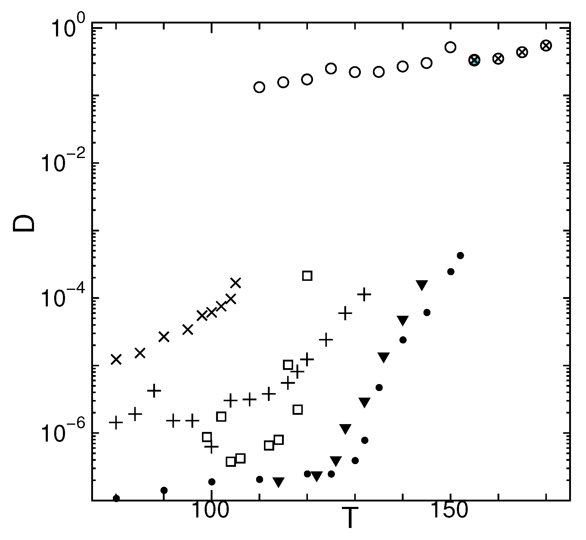
In Figure 1, the temperature dependence of the diffusion coefficient D (time average of MSD) for different states is shown. The melting temperature is in the investigated system. For non diffusive states, the MSD is often stepwise/oscillatory as shown in the following subsections. The determination of D will be difficult in such situation. In principle, D should be determined in a time scale (or length scale) where MSD becomes linear against time. Nevertheless, we make a linear fit to the MSD data against time shown in the MSD figures in the following Section 2.2, Section 2.3, Section 2.4 and Section 2.5 and calculate D (except otherwise stated). Because of this strong non-linearity, especially at low temperatures, the variance of D are temperature dependent and larger for lower temperatures in general. When a clear change in the nature of MSD occurs during a simulation at a certain fixed temperature, the values of MSD after that clear change are only used for calculating D. Such a situation occurs in state J at , 106, and 118 (see Section 2.3). See Appendix A.4 for calculation details of MSD.
For the metastable states, an inflection temperature is observed where D increases drastically. We define the temperature where D starts to increase drastically as and use it as a reference temperature to denote the dynamical change. In experimental findings, is correlated to the glass transition temperature [21,22,23,24,25,26,27]. For crystals at temperatures , slight diffusion is observed. However, in this temperature range, no particles escape from the region beyond the 1st nearest neighbor in a certain time duration (see Figure 2). For temperatures , hopping occurs in the crystal. However, it occurs in a spatially isotropic manner in contrast to the metastable glassy states which often show anisotropic hopping. Note that the diffusion resulting from the hopping dynamics in crystal become notably large near the melting transition at .
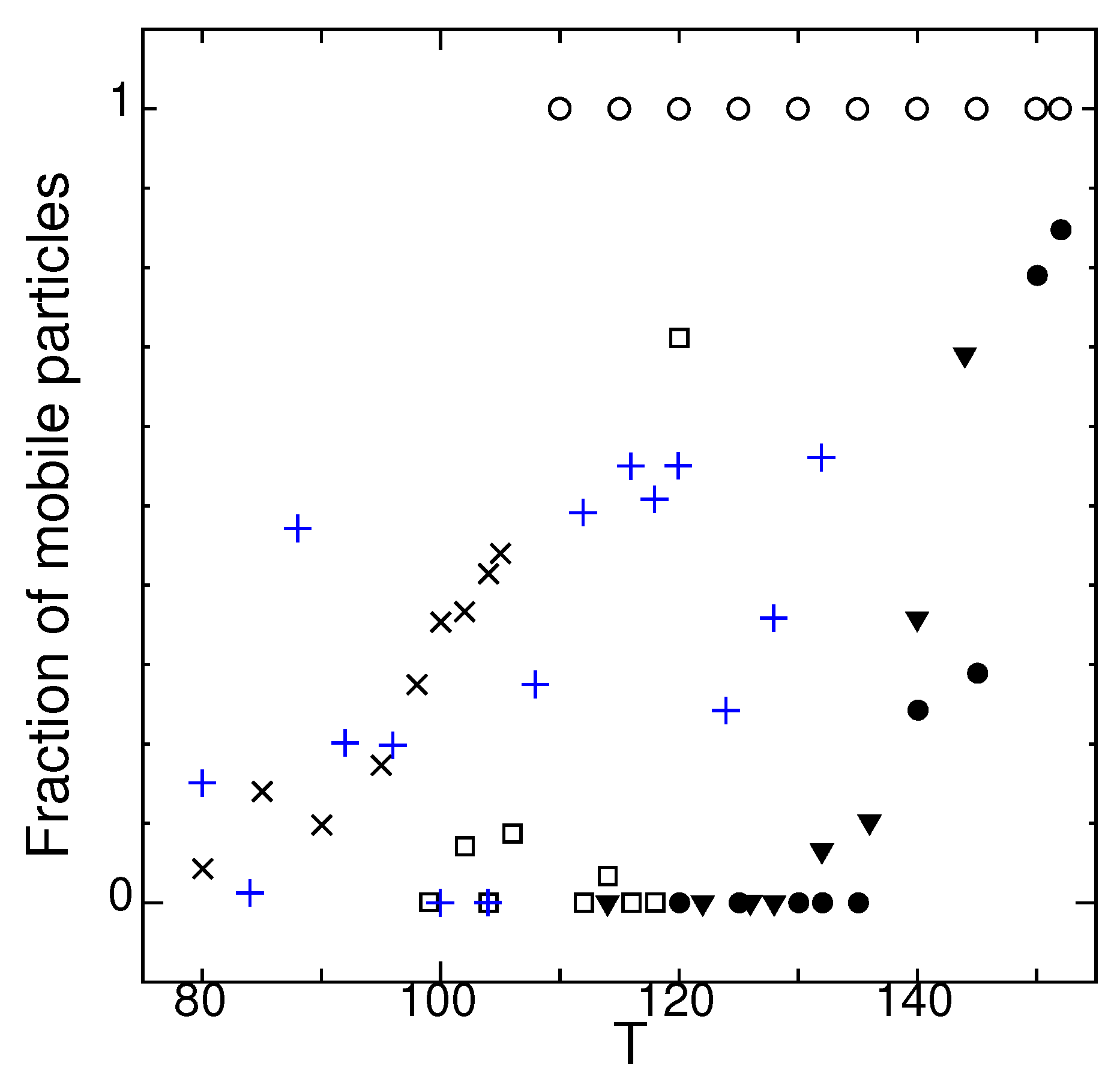
In Figure 2, the temperature dependence of the fraction of mobile particles for each state is shown. The number of particles which move more than the average excluded volume length (effective core) in time duration are defined as mobile. See Appendix A for the definition of . Note that the measurement time for Figure 2 is limited compared to measurement of MSD and of D in Figure 1.
In state O (symbol blue +), there is a slow oscillation in MSDs at low temperatures where collective movements of particles occur beyond the measuring time. The fluctuation in the values of state O in Figure 2 is due to the choice of measuring time because of the slow oscillating nature of MSD of state O. See Section 2.5 for details.
2.2. State G
State G has the lowest diffusion constant D among the metastable states for a wide range of temperature.
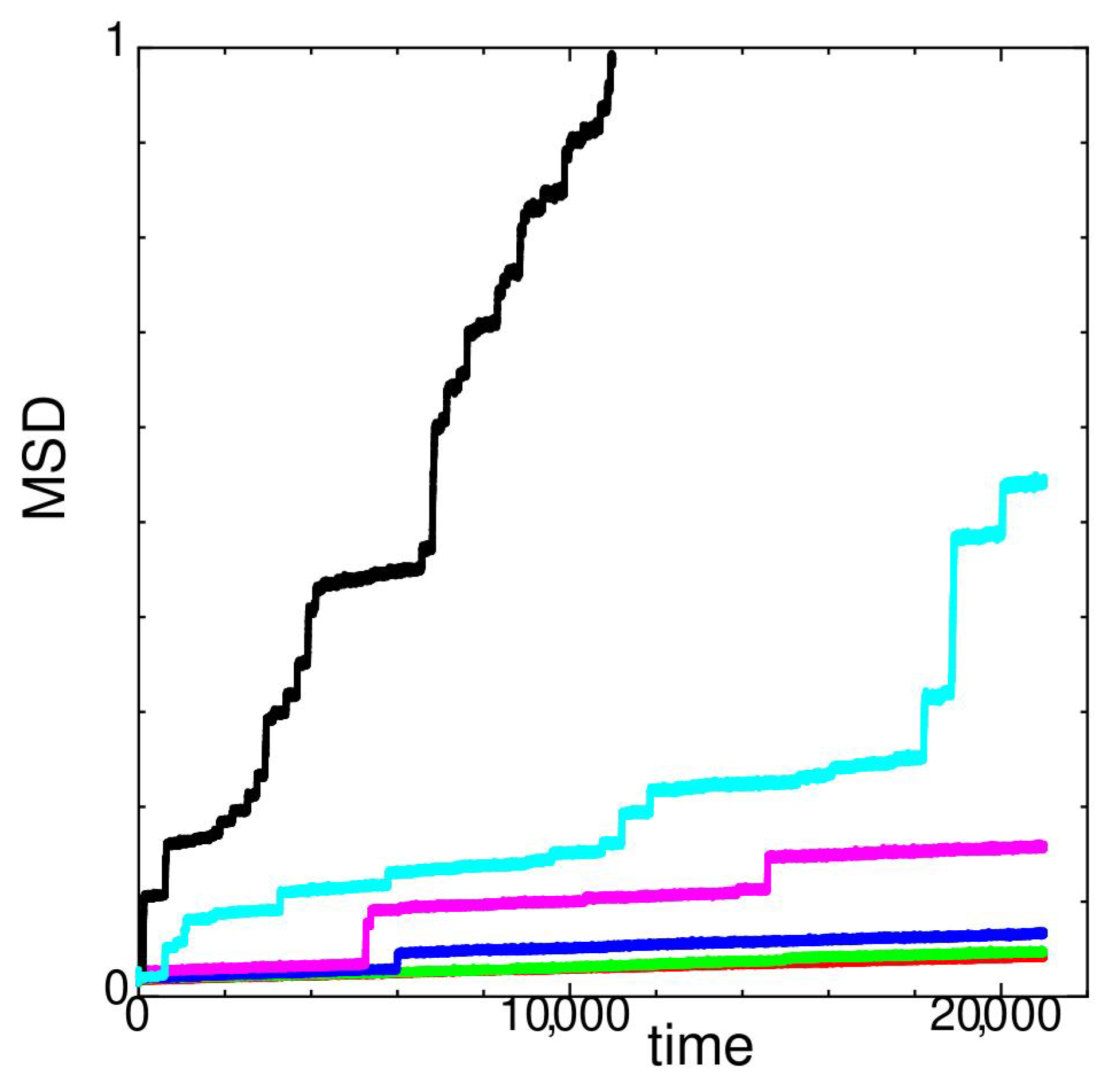
In Figure 3, MSD of state G versus time at different temperatures is shown.
At temperatures and , MSD changes only slightly. A stepwise increase in MSD is observed at . This is because the values of MSD are extremely small and the hopping nature of individual particles appears in Figure 3. Most of the glassy states of monodispersed softcore systems show hopping diffusion [8,9].
2.3. State J
State J shows intermittent structural rearrangements.
State J has been first obtained as a result of spontaneous structural transformation of state H at in the original system size [9]. The initial configuration of state H is the amorphous solid state reported in Figure 12 of [13]. During the calculation of state H at , the volume and the total potential energy decreased and transformed to J state [9]. The physical properties of H and J states are are completely distinct and the pair distribution function shows a clear structural transformation. State H is stable for temperature regions and . See Figure 3 of [9] for other structural transformations observed in WCA spheres. These facts show that the connectivity of basins and their depth for these metastable states are temperature dependent.
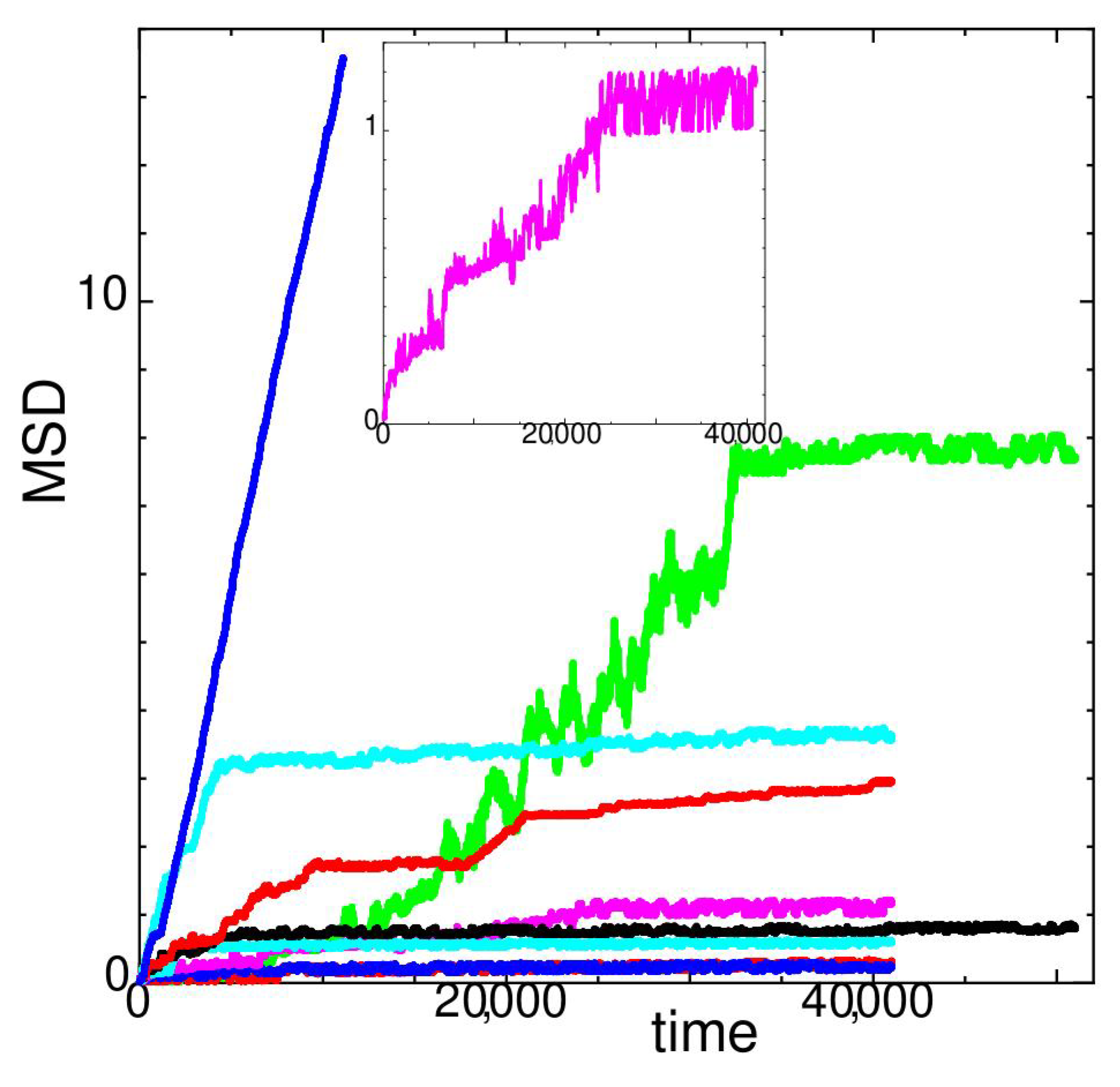
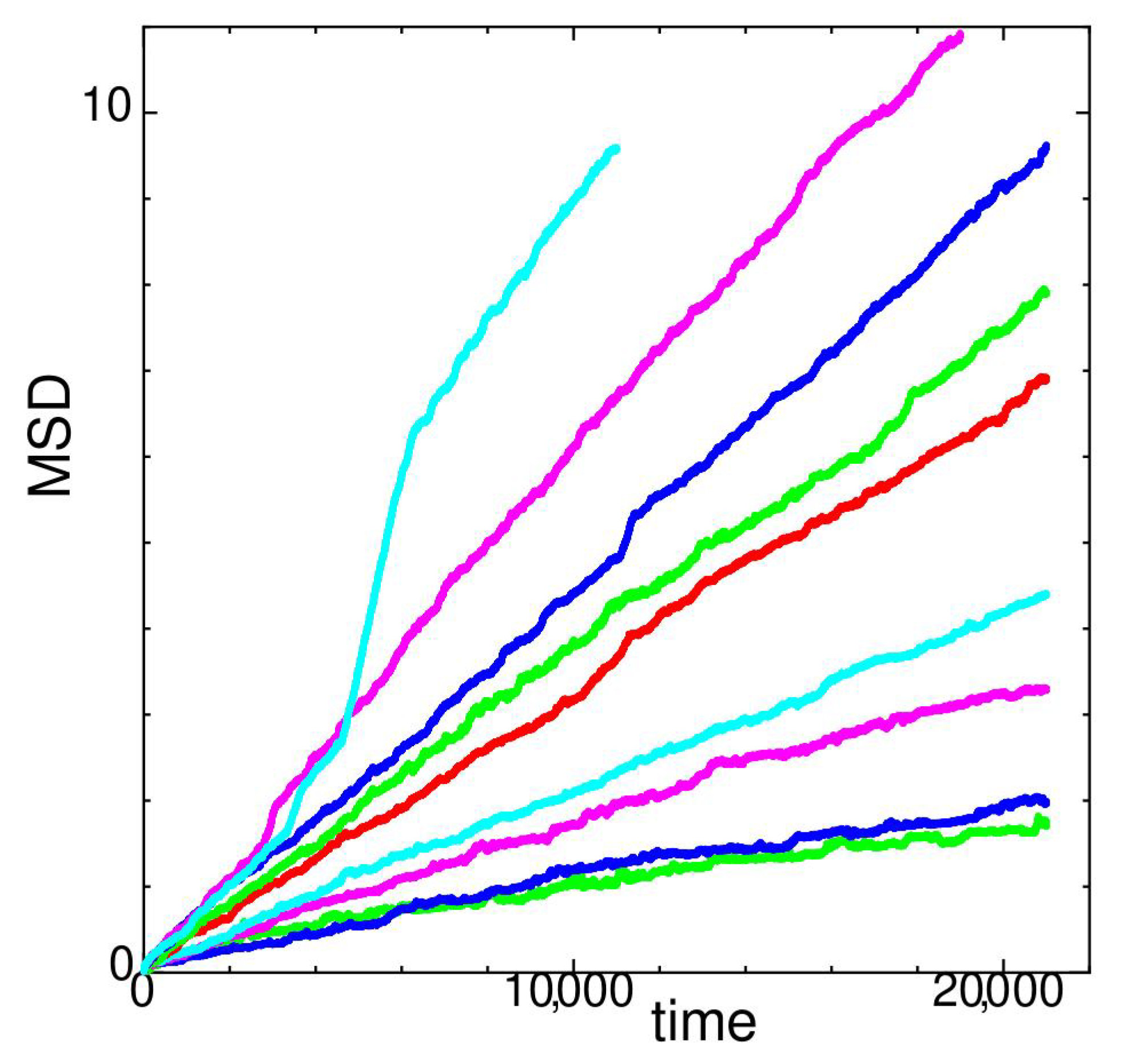
In Figure 4, the MSD of state J versus time at different temperatures is shown. For system size reported here, state J seems to be relatively unstable at temperatures .
At (cyan with larger MSD values), MSD rapidly increases at the beginning; however, it slows down to a constant rate. The diffusion constant D at in Figure 1 is calculated for 41,000. At (larger red values), a stepwise nature due to hopping appears in the MSD. At (magenta, also shown in the inset of Figure 4), string-like hopping motion occurs; however, the rate decreases at t > 24,000. In Figure 1, D is calculated at 24,000 < 41,000 for . At (green), MSD drastically increases upto but both the diffusion and the fluctuation become much smaller at larger times. A landslide in the stacking layer occurs before that time and results in a structural transformation. At , the diffusion constant D shown in Figure 1 is calculated at 32,500 < 51,000. For other temperatures not mentioned above, the diffusion constant D in Figure 1 is obtained by averaging through the whole measuring time. At temperature , MSD increases drastically compared to lower temperatures.
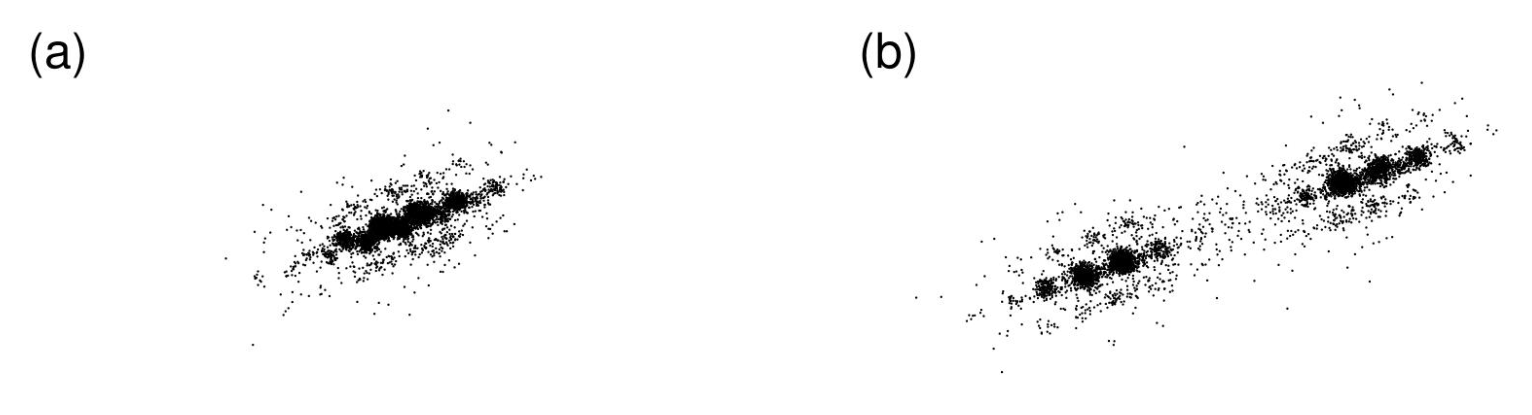
In Figure 5, displacement plots of state J at and at times (a) , and (b) are shown. The MSD shows large fluctuation and increase before (green line in Figure 4). Displacement plots show positions relative from the initial position of all particles projected on a plane. Thus, displacement plots reveal spatially cooperative movements. A straight string-like hopping motion can be clearly discerned in Figure 5. In addition, the center crowded position where particles are fluctuating around the original position, splits into two as shown in Figure 5b. A landslide occurred between the time shown in Figure 5a,b. The length scale of the landslide is about six times larger than the distance of the neighboring particles (see Supplementary Material).
The phenomenon where the displacement center splits into two (along with string-like motion) is also observed at temperature of state J for system size . Thus, state J in this temperature range seems to be susceptible to landslides, due to the small elastic modulus (see Section 3 for further discussion).
2.4. State M
State M is the most diffusive state among the metastable states studied in this paper. A clear temperature dependence of MSD is observed for state M as shown in Figure 6.
The inflection point in the increment of D observed in logscale (Figure 1) is not so clear compared to other states.
2.5. State O
State O is a state with a long trajectory reversal time and distance.
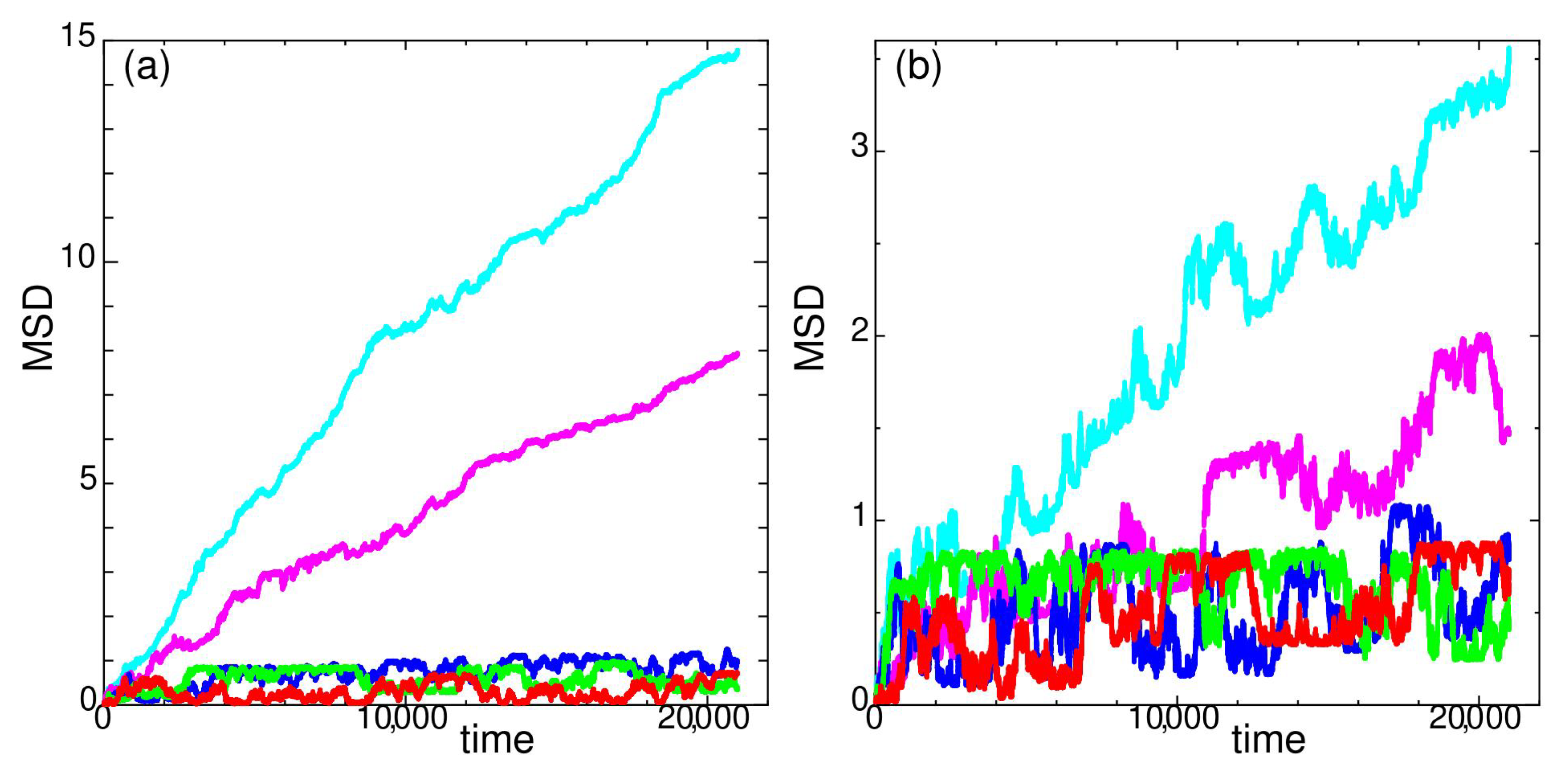
In Figure 7, MSD of state O is shown. The overall temperature dependency is shown in Figure 7a. At and 132, the system is quite diffusive. For temperatures , MSD of state O shows a long time fluctuation with a large return distance as clearly seen in Figure 7b.
A large oscillation in the MSD shows that there is a collective movement among the particles. This collective movement clearly appears in the self-van Hove correlation function,
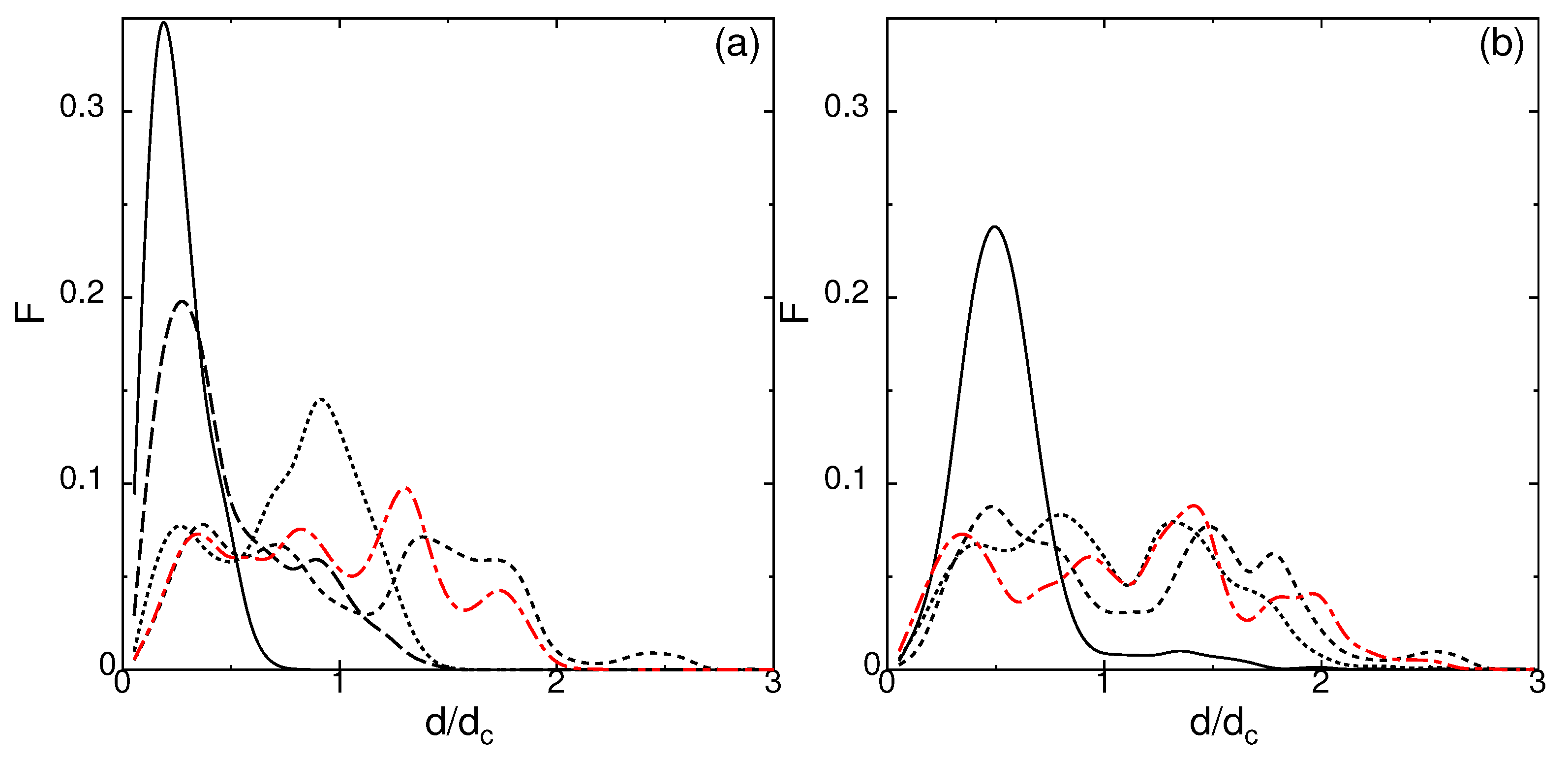
which is the probability of displacement d in duration of time , where and are the position of particle i at time t and at , the origin of the measurement. In Figure 8, the self-van Hove correlation functions measured at several time duration against the distance scaled by the effective core length are shown.
Since the large fluctuation of MSD seems quite random but is confined in a certain width for state O (Figure 7b), the self-van Hove correlation function depends not only on the time duration , but also on the absolute time where the measurement is taken. To show the effect of time duration alone, the finishing time of the measurement is common in Figure 8 except for the red dot-dashed line. The fraction of mobile particles (Figure 2) and elastic properties (Section 3) for state O are taken at the same time duration t = 20,000–21,000 shown by the red dot-dashed line. It is clear from Figure 8 why the fraction of mobile particles are high at and 116 in Figure 2. At the time duration t = 20,000–21,000 where the measurements of Figure 2 are done, particles are scattered to relatively large distances, which tend to return close to their original positions at longer time duration as shown by the solid line in Figure 8a,b. Figure 8 clearly shows that the distance for trajectory reversal (rattling distance) extends beyond twice the distance . The time scale differences between the trajectory reversal motion and diffusive motion clearly appear in the MSD at low temperatures (Figure 7b). State O has a large return distance regardless of system size and the same characteristics are persistently observed in other system sizes and 2688.
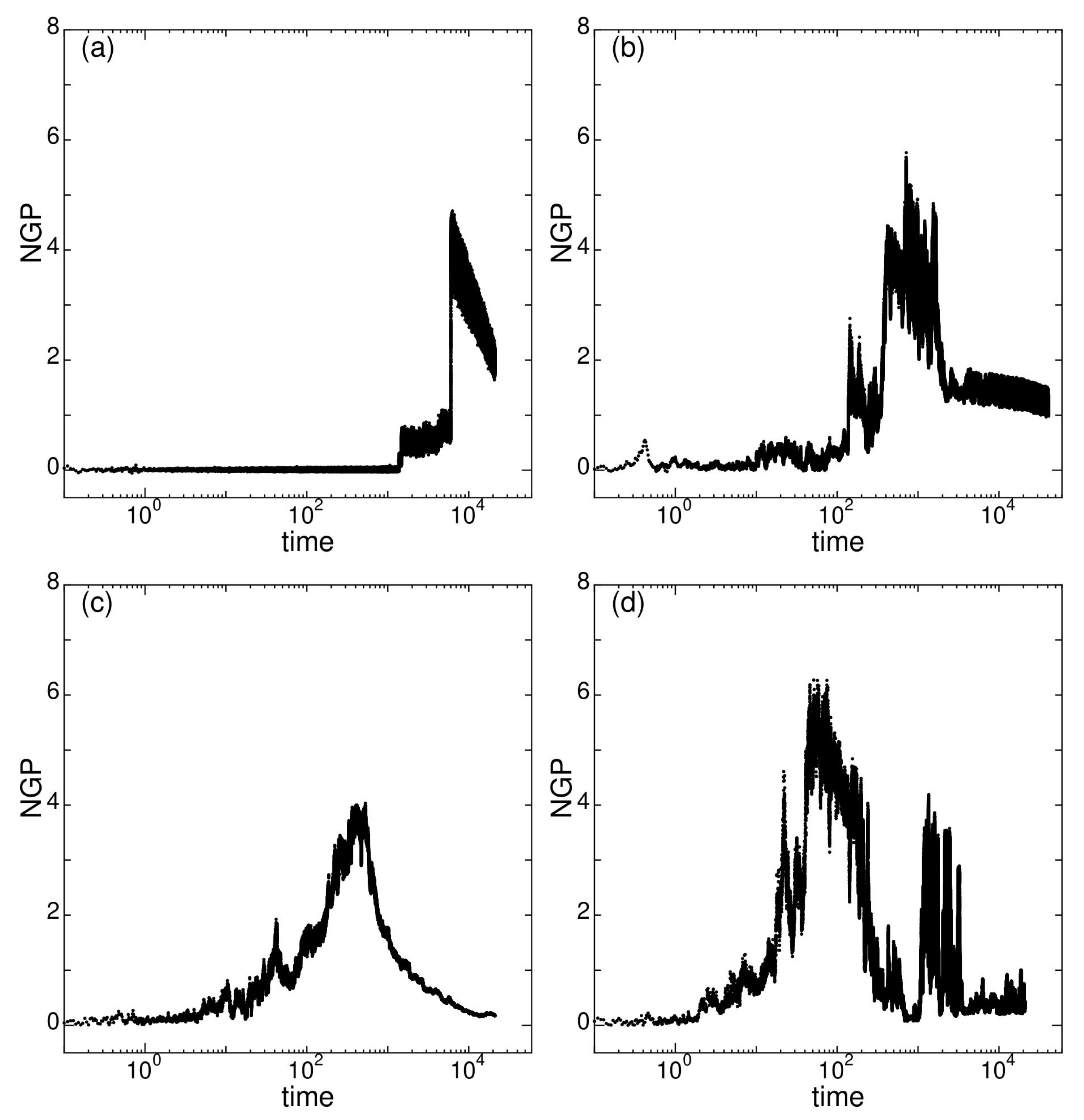
2.6. Dynamical Heterogeneity at
The dynamical heterogeneity is a phenomenon where dynamically active and inactive regions appear in the same system. To measure the degree of dynamical heterogeneity, the non-Gaussian parameter(NGP) is calculated. NGP is defined as
where l is the dimension, is the displacement of the particles in duration of time t and is the MSD. The NGP plotted against time will show the degree and time scale of the dynamical heterogeneity.
In Figure 9, the three dimensional () NGP near is shown. In state G (Figure 9a), NGP become notably positive after , where a sharp asymmetric peak appear near . The calculated time is not enough to observe whether the decay is linearly falling off. For state J (Figure 9b), the decay of NGP is very slow and show large fluctuation. The NGP curve of state M (Figure 9c) resembles that of colloidal glasses in experimental observations [28,29,30,31,32]. Reflecting the large particle reversal movements in state O, the NGP curve (Figure 9d) shows two separated large peaks, consisting of smaller peaks. All the states show distinctively different characteristics in the NGP curves, which reveals that the nature of dynamical heterogeneity is different for each state.
3. Elastic Properties
To calculate elastic properties, spontaneous stress and strain in longitudinal and transverse directions are measured. For calculation details, see Appendix A.5.
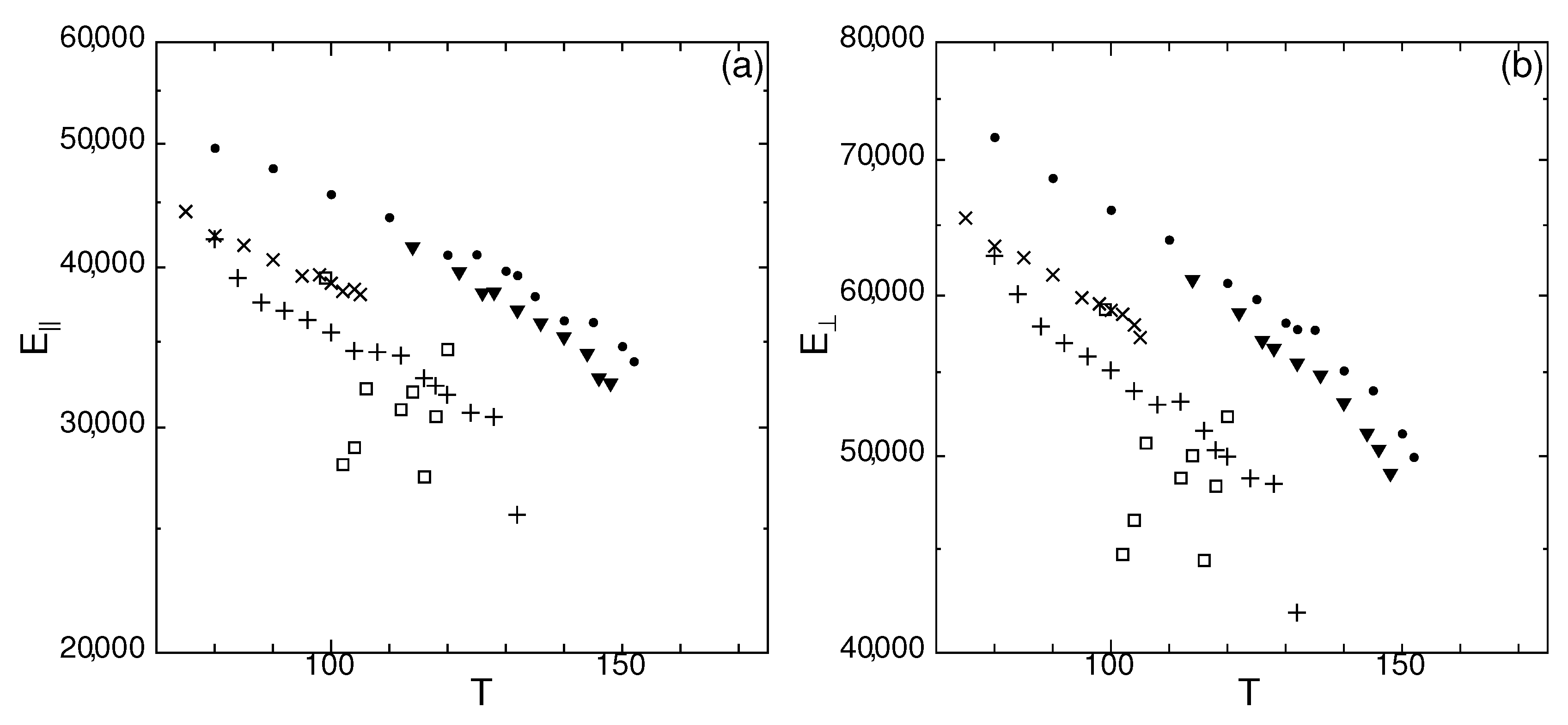
3.1. Temperature Dependence of Modulus of Spontaneous Elastic Tension/Compression
In Figure 10, the temperature dependence of the longitudinal and transverse elastic modulus is shown. All states, except state J, elastic modulus and in log-scale show approximately a linear dependence on T. Only state O shows a tendency of softening at . Note that the sharp increase in D occurs around for state O (Figure 1), revealing that the elastic properties stay intact even at higher temperatures where the particles get mobile.
For state J, the values are scattered in Figure 10, and difficult to discern a relation against T. Note that at the calculated lowest and highest temperatures ( and 120) of state J, the values of and are higher than other temperatures and overlap with the value of state M at . As discussed in Section 2.3, MSD at , 106, and 118 showed peculiar characteristics and D was calculated for a limited time at the end of the simulation. At which mark the 2nd smallest values of and of state J, a landslide was observed (Figure 5). The fraction of mobile particles of state J was high only for . For other states, the temperature dependence of and is not affected even at temperatures higher than where the particles get mobile. For supercooled liquids, and are at least two orders of magnitude smaller than other metastable states, thus not shown in Figure 10.
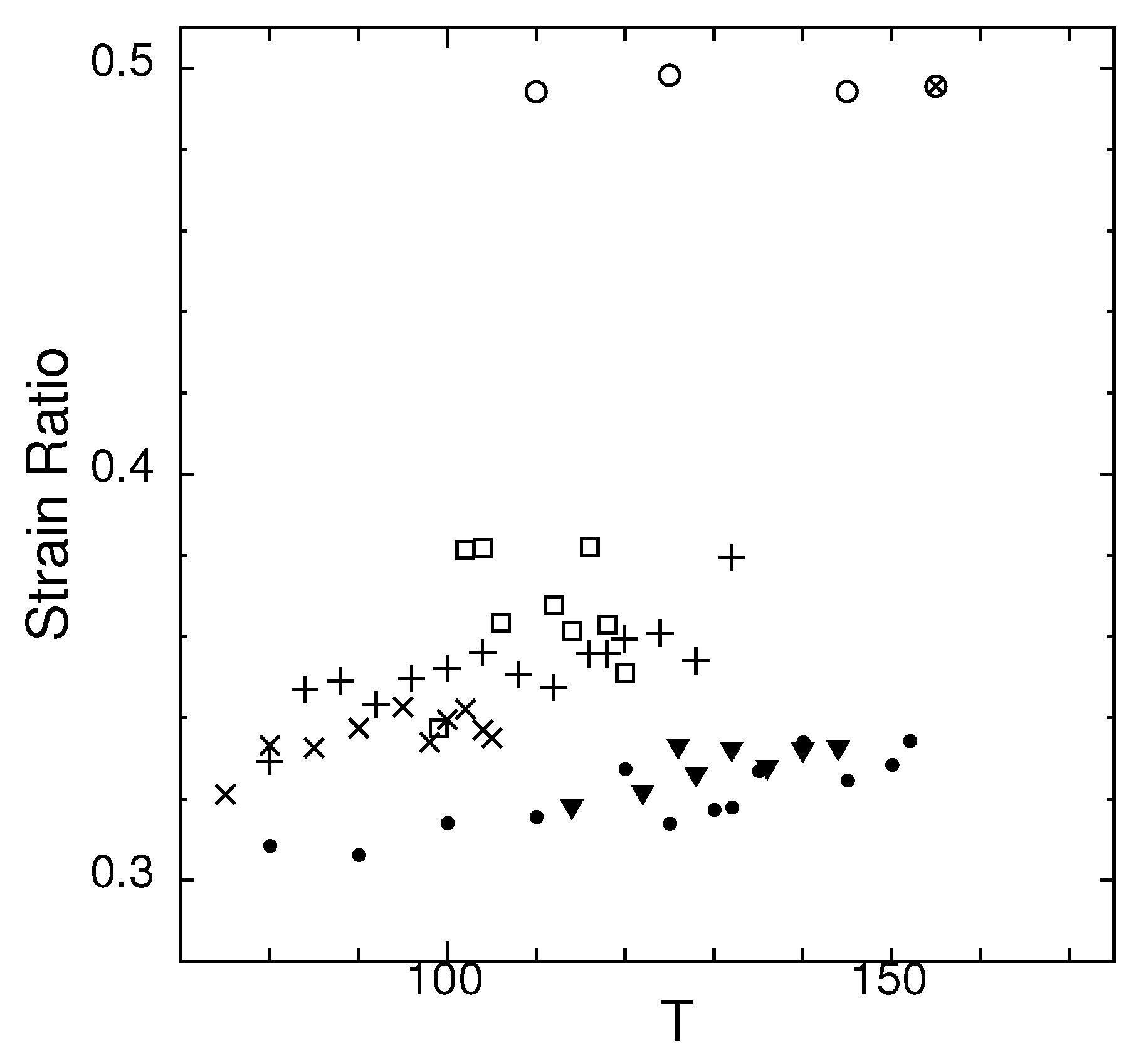
3.2. Temperature Dependence Spontaneous Strain Ratio
In Figure 11, the ratio of spontaneous strains are plotted against temperature.
For comparison, some data for the supercooled and thermodynamic equilibrium liquids are also shown. The strain ratios are for the liquids, like the Poisson’s ratio [33,34,35]. The relation between elastic modulus for isotropic medium is
This equation shows that as , the shear modulus S drastically decreases if the change in bulk modulus is small [36]. We show, in the next section, that the bulk moduli in supercooled and equilibrium liquids have a smaller temperature dependence compared to the metastable states, thus indicate that shear modulus at melting.
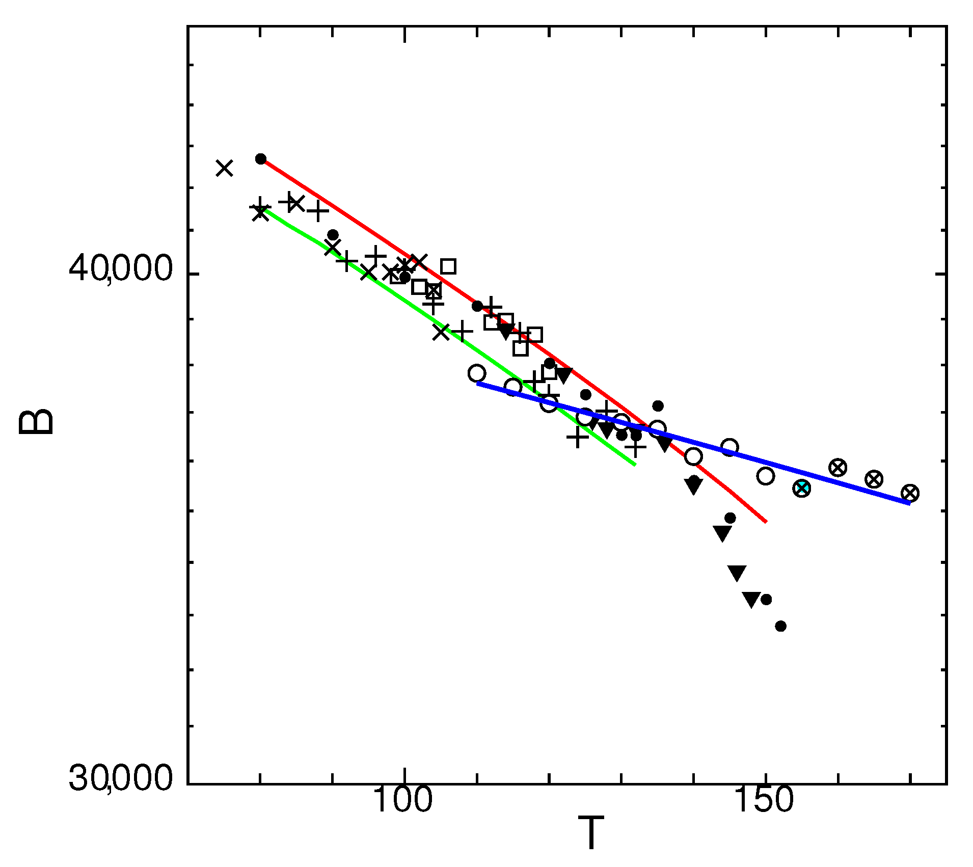
3.3. Temperature Dependence of Spontaneous Bulk Modulus
In Figure 12, temperature dependence of bulk modulus for the glassy states and liquids is shown.
Finite-strain theory has been applied extensively to problems in geophysics. The theory relates compression/expansion to pressure. The Birch–Murnaghan equation of state [37] in the second degree is,
where , V is the volume at P, and the bulk modulus is that of volume at a reference pressure . This semi-empirical Equation (4) requires a reference value of the bulk modulus for volume to be determined from experiment. In geophysics, the reference values are usually those at the ambient pressure. Using the above Relation (4), the temperature dependence of the bulk modulus is
The temperature dependence of bulk modulus B of glassy states are fit to Equation (5). The reference values and are taken from the values at for crystal (red line) and state M (green line).
Most of the glassy states conform to Equation (5) obtained from the Birch–Murnaghan equation of state and fit between the region inside the red and green lines. However, when the temperatures get closer to the melting transition, the crystal state (•) becomes drastically softer than Equation (5) predict. In contrast, the temperature dependence of the liquids (blue line) is small and do not decrease drastically for temperatures higher than the melting temperature . This conforms to the fact that when the Poisson’s ratio is close to , the change in bulk modulus is small [36].
4. Concluding Remarks
Molecular dynamic simulations which allow anisotropic fluctuations of the cell shape to preserve hydrostatic pressure have been conducted. Using a simple monodispersed model, we have shown that below the melting temperature , there exists multiple metastable states with distinctive dynamics. They are glassy metastable states where diffusion constants increase sharply at a certain temperature . Around , dynamic heterogeneity is observed. The drastic increase in diffusion constants at does not induce change in the temperature dependence of the elastic modulus. The elastic properties show that these metastable states are basically solids even at temperatures higher than . The rigidity and mobility of glassy metastable states are compatible even at higher temperatures than . There exists a rigid supporting framework which allows other parts to flow. Because of this framework, dynamical heterogeneity is sustained. How to quantitatively assess these structures, especially the supporting framework, will be addressed in future work. The bulk moduli for the supercooled/equilibrium liquids only show a slight temperature dependence compared to glassy metastable states.
Once we admit that there exist multiple metastable solid states with glassy dynamics, the scenario behind polyamorphous and liquid–liquid transition [38,39,40,41,42,43,44,45] will attain many possibilities. The temperature range of each metastable state might be different; thus, beyond those bounded temperatures, the state is destined to transform to another state. These transformations may also occur among two diffusive states. In the original system, we observed a clear change in MSD at a transformation among two different states (see Figure 11 of [8]). To address these important subjects, not only simulations of larger systems near as performed here, but also in the whole temperature range, especially towards , is needed and remain for future work.
Supplementary Materials
The following are available online at https://0-www-mdpi-com.brum.beds.ac.uk/article/10.3390/solids2020016/s1, Figure S1: Snapshots of state J at T = 102 viewed on 3 different planes (xy-, xz-, and yz-plane) at (a) t = 11,100, (b) t = 32,400, and (c) t = 51,000, respectively. Colors depend on the z-coordinate at t = 51,000 to show where the particles originate in former times. Particles are depicted small to show the position clearly. (a) yz-plain (right) clearly show a landslide (with two layers paired to slide approximately 6 times that of normal direction between the layers) have settled into the final layered positions at (c).
Funding
This research was supported by JSPS KAKENHI Grant No. JP17K05589.
Acknowledgments
This paper was written in memory of Professor Fumiko Yonezawa. The author is grateful to Professors Shuhei Ohnishi, Kiyoshi Sogo and Susumu Fujiwara for valuable discussions.
Conflicts of Interest
The author declares no conflict of interest.
Appendix A. Computer Simulation Methods
The principle of corresponding states [46] holds for systems with simple pair-wise interaction, i.e., the inter-particle potential having the functional form . By introducing the mass m, length , and energy , as fundamental units, other physical quantities may be defined by them; such as pressure , temperature , and molecular volume . Under these reduced units, a thermodynamic state point determines a set of corresponding states which applies to thermodynamics, structural, and dynamic properties [47].
Furthermore, if particles interact by repulsive force alone, a single reduced variable defines the excess properties. For inverse power potential , the reduced density determine the state. A single isotherm, isochore, or isobar is sufficient to determine the entire phase diagram of thermodynamic equilibrium [48]. This can be understood as the average excluded distance of a pair of particles (the effective core) equals the average kinetic energy [14] defined by the systems temperature T, i.e., . It reveals that the temperature dependence of the effective excluded volume is the crucial factor. Similarly, for the WCA potential, the relation
will determine the effective core at temperature T. Again, the temperature dependence of excluded volume is the crucial factor. Even when there is anisotropy in the shape of the particle, similar comprehension leads to the scaling law of the system [49]. The equation of state under the reduced units for these simple models will be given by plotted against density, where ; expressed by the inverse function of the pair potential .
Appendix A.1. Symplectic Integrator for Soft Matter
To properly investigate thermodynamic and dynamic properties of condensed matter, the system should not be under non-hydrostatic stress. To achieve simulations under hydrostatic pressure, not only the volume but also the shape of the simulation cell must change according to the stress tensor caused by the constituent particles. In the method used in this work, the shape and size of the simulation cell is described by an anisotropic factor and an isotropic volume factor Q where the volume of the simulation cell is [13]. The anisotropic factor is the ratio of the simulation cell lengths in z and xy-directions (length in x and y-directions are the same in this study), i.e., . The isotropic volume factor Q expands and contracts isotropically, while expresses the change in shape. These variables and Q change spontaneously, evolving the system towards hydrostatic pressure with the scalar pressure balancing with the given value . Periodic boundary conditions are applied to x, y, and z directions. In this method, the Hamiltonian is solved by a symplectic integrator which preserves the structure of the Hamilton’s equations of motion. Thus, high precision and stable trajectory is guarantied. System size effects are small in this method and notable only near the phase transition. See Figure 6 of [50].
Appendix A.2. Calculation of Metastable States
All the metastable states investigated in this paper are morphologically changed from the pristine forms of the amorphous solid or supercooled liquid reported in [13] to settle in a basin under isothermal and hydrostatic pressure. That is the basin of the free energy profile of the total system where the crystal state is in the global minimum and metastable states are in local minima. The value of the given pressure in these simulation has an effect on the sharpness of the transition. When is high, the melting transition temperature becomes high, thus leading to a smaller near . Since the potential becomes steeper when becomes smaller, the particles are effectively harder at higher pressures. The potential landscape becomes steeper as well.
To seek the stable temperature range of a certain metastable state, a series of calculations at different temperatures are done independently from a common initial configuration. During these calculations, we occasionally observe the system transform to a different state. Some examples of such structural transformation are given in Figure 3 of [9]. The transformation occurs in a short time duration, compared to the calculated time. Such transformations are caused by a rare event knocking the system over the energy barrier to a new state. Information of the free energy profile of WCA phase space, such as the approximate depth of the basin, is obtained through such calculations. Occurrence of such transformation not only appears in the static values, but also in the dynamics such as the MSD.
Appendix A.3. Model and Initial Configurations
To investigate to what extent the excluded volume effect alone can describe the properties of glass, soft isotropic monodispersed spheres are employed as a model system. Pairwise potential of WCA [12] is used. Reduced units are employed throughout our work. In addition to the metastable states explained below, the dynamic and elastic properties of crystalline solid are investigated for comparison. The given pressure is set to where the melting temperature from equilibrium crystalline solid to liquid is . The effective particle size at the melting temperature is .
Metastable states for monodispersed WCA spheres are initially reported in [13] as amorphous solids. A total of seventeen states, including the supercooled liquid, are reported in [8,9]. Among them, four states in [9] are chosen, i.e., states G, J, M, and O; the labels of each state will remain the same as the original article to avoid confusion. The original calculations were done for number of particles . In this work, the configuration of these states were stacked four times and used as the initial configuration for a new system size . The initial configurations to construct the system, are those of ; states G, J, M, and O at temperatures , 100, 104, and 106, respectively, at which these states were first identified [13].
Note that the supercooled liquids reported here are metastable states obtained independently at each temperature where the thermal fluctuation cannot overcome the energy barrier at each temperature in the calculated time. The supercooled liquid exists as a thermodynamic metastable state at for the original system size . At lower temperatures, solidification occur and marked by a clear change in MSD and the volume/density [8]. The supercooled liquid is calculated for for system size where the typical total calculation time is to 6000. The initial configuration was the original system (of at ) stacked four times. For crystalline solid, data at of was used to construct the initial configuration. The crystalline state of was calculated to at and did not melt.
The mass of the barostat is and the mass of the thermostat is throughout this work. All calculations were done with time step .
Appendix A.4. Calculation of Transport Coefficient
A linear fit to the mean square displacement against time gives the diffusion constant D.
Since the velocity of each particle i is calculated at every time step for the molecular dynamics, the displacements calculated from the velocities (in each direction ) are tracked along the time evolution and used for calculating the transport properties. This allows the calculation of transport properties unaffected by the periodic boundary conditions.
Appendix A.5. Calculation of Elastic Properties
The spontaneous elastic modulus for each state are calculated from the stress versus strain plot as in [51]. Although we do not have any uniaxial load in our simulation, the geometry of the spontaneous fluctuations is those of Poisson’s ratio measurements [33,34]. Instead of a uniaxial load, we have a spontaneous uniaxial shape fluctuation (in addition to the volume fluctuation) of the simulation cell where the strains can be directly measured. Simultaneously, the internal stress tensor is tracked by the simulation method. The longitudinal and transverse strains/stresses can be measured regardless of the state of matter in our method. The isotropic volume factor Q is related to the cell length in x and y-direction by , and will give a modulus of spontaneous elastic tension/compression. This modulus is calculated by plotting the transverse stress against the transverse strain . Similarly, the uniaxial elastic modulus is obtained from longitudinal stress and longitudinal strain . Values of the transverse strain against longitudinal strain give the spontaneous stress ratio. The instantaneous stress and strain are measured at each (100 time steps) for a time duration of ( time steps) at the end of each simulation. The modulus of volume expansion/contraction (the spontaneous bulk modulus) is calculated from collecting the instantaneous values of mean stress and strain of the simulation cell. The elastic modulus and the strain ratio are calculated when the cell shape is relatively stable for time duration , otherwise we only calculate the bulk modulus.
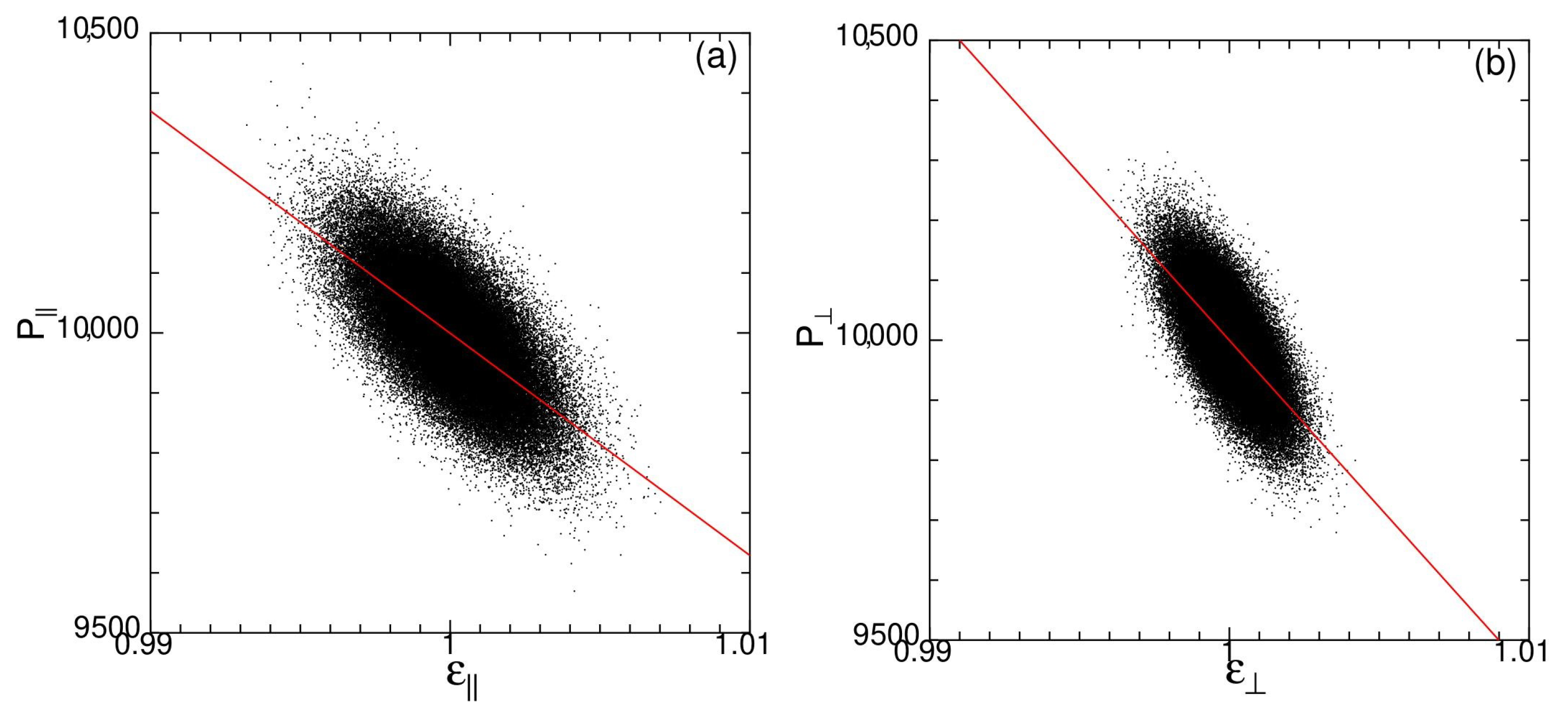
In Figure A1, the spontaneous stress and strain are plotted for state G at temperature . Each dot represents an instantaneous value measured at 20,000 < 21,000. Red lines are the linear fit to all points. In the strain–stress plot, the data points form a ellipse showing that the state is viscoelastic to some extent. Nevertheless, we make a linear fit to all data points. For Figure A1, the red line which is the linear fit to all points does not go through the middle of area of dots. This is because data points are more distributed on the high-strain/low-stress area which shows that it is more difficult to compress than to expand in this system.
Figure A1.
Spontaneous stress and strain of state G for time duration at temperature : (a) longitudinal stress versus strain, (b) transverse stress versus strain, (c) bulk stress versus strain, and (d) ratio between transverse and longitudinal strains, for system size . Red lines are the linear fit to all points.


References
- Shelby, J.E. Introduction to Glass Science and Technology, 2nd ed.; The Royal Society of Chemistry: Cambridge, UK, 2005. [Google Scholar]
- Bernu, B.; Hiwatari, Y.; Hansen, J.P. Soft-sphere model for the glass transition in binary alloys: Pair structure and self-diffusion. J. Phys. C 1985, 18, L371. [Google Scholar] [CrossRef]
- Wahnström, G. Molecular-dynamics study of a supercooled two-component Lennard-Jones system. Phys. Rev. A 1991, 44, 3752. [Google Scholar] [CrossRef]
- Kob, W.; Andersen, H.C. Testing mode-coupling theory for a supercooled binary Lennard-Jones mixture I: The van Hove correlation function. Phy. Rev. E 1995, 51, 4626. [Google Scholar] [CrossRef] [Green Version]
- Sollich, P. Predicting phase equilibria in polydisperse systems. J. Phys. Condens. Matter 2002, 14, R79–R117. [Google Scholar] [CrossRef]
- Brazhkin, V.V. Can high pressure experiments shed light on the puzzles of glass transition? The problem of extrapolation. J. Phys. Condens. Matter 2008, 20, 244102. [Google Scholar] [CrossRef]
- Angell, C.A.; Borick, S. Specific heats Cp, Cv, Cconf and energy landscapes of glass forming liquids. J. Non-Cryst. Solids 2002, 307–310, 393–406. [Google Scholar] [CrossRef] [Green Version]
- Aoki, K.M.; Fujiwara, S.; Sogo, K.; Ohnishi, S.; Yamamoto, T. One-, Two-, and Three-dimentional Hopping Dynamics. Crystals 2013, 3, 315–332. [Google Scholar] [CrossRef]
- Aoki, K.M.; Fujiwara, S.; Sogo, K.; Ohnishi, S.; Yamamoto, T. Molecular Dynamics Simulations of One-, Two-, Three-dimensional Hopping Dynamics. JPS Conf. Proc. 2014, 1, 012038. [Google Scholar]
- Aoki, K.M.; Yoneya, M. Order Parameter Discretization in Metastable States of Hexatic Smectic B Liquid Crystal. J. Phys. Soc. Jpn. 2011, 80, 124603. [Google Scholar] [CrossRef]
- Aoki, K.M. Network Analysis of Free Energy Landscaper of Metastable States of Hexatic Smectic B Liquid Crystal. J. Phys. Soc. Jpn. 2014, 83, 104603. [Google Scholar] [CrossRef]
- Weeks, J.D.; Chandler, D.; Andersen, H.C. Role of Repulsive Forces in Determinig the Equilibrium Structure of Simple Liquids. J. Chem. Phys. 1971, 54, 5237. [Google Scholar] [CrossRef]
- Aoki, K.M. Symplectic Integrator Designed for Simulating Soft Matter. J. Phys. Soc. Jpn. 2008, 77, 044003. [Google Scholar] [CrossRef]
- Aoki, K.M. Molecular Dynamics Simulation of Anisotropic Molecules as a Model of Liquid Crystals. Ph.D. Thesis, Keio University, Yokohama, Japan, 1993. [Google Scholar]
- Aoki, K.M.; Yoneya, M.; Yokoyama, H. Extended methods of molecular dynamics simulations under hydrostatic pressure and/or isostress. J. Chem. Phys. 2003, 118, 9926. [Google Scholar] [CrossRef]
- Aoki, K.M.; Yoneya, M.; Yokoyama, H. Molecular dynamics simulation methods for anisotropic liquids. J. Chem. Phys. 2004, 120, 5576. [Google Scholar] [CrossRef]
- Aoki, K.M.; Yoneya, M.; Yokoyama, H. Constant surface-tension molecular-dynamics simulation methods for anisotropic systems. J. Chem. Phys. 2006, 124, 064705. [Google Scholar] [CrossRef]
- Aoki, K.M. Anisotropy in condensed matter - liquid crystals, glass, and phase coexistence. J. Phys. Conf. Ser. 2019, 1252, 012004. [Google Scholar] [CrossRef] [Green Version]
- Abraham, S.; Harrowell, P. The origin of persistent shear stress in supercooled liquids. J. Chem. Phys. 2012, 137, 014506. [Google Scholar] [CrossRef] [PubMed] [Green Version]
- Fuereder, I.; Ig, P.I. Influence of inherent structure shear stress of supercooled liquids on their shear moduli. J. Chem. Phys. 2015, 142, 144505. [Google Scholar] [CrossRef] [Green Version]
- Petry, W.; Bartsch, E.; Fujara, F.; Kiebel, M.; Sillescu, H.; Frago, B. Dynamic anomaly in glass transition region of orthoterphenyl. Z. Phys. B Condens. Matter 1991, 83, 175–184. [Google Scholar] [CrossRef]
- Buchenau, U.; Zorn, R. A Relation between Fast and Slow Motions in Glassy and Liquid Selenium. EuroPhys. Lett. 1992, 18, 523–528. [Google Scholar] [CrossRef]
- Angell, C.A. Formation of Glasses from Liquids and Biopolymers. Science 1995, 267, 1924–1939. [Google Scholar] [CrossRef] [PubMed] [Green Version]
- Magazù, S.; Maisano, G.; Migliardo, F.; Mondelli, C. Mean-Square Displacement Relationship in Bioprotectant Systems by Elastic Neutron Scattering. Biophys. J. 2004, 86, 3241–3249. [Google Scholar] [CrossRef] [Green Version]
- Niss, K.; Dalle-Ferrier, C.; Frick, B.; Russo, D.; Dyre, J.; Alba-Simionesco, C. Connection between slow and fast dynamics of molecular liquids around the glass transition. Phy. Rev. E 2010, 82, 021508. [Google Scholar] [CrossRef] [Green Version]
- Capaccioli, S.; Ngai, K.L.; Ancherbak, S.; Paciaroni, A. Evidence of Coexistence of Change of Caged Dynamics at Tg and the Dynamic Transion at Td in Solvated Proteins. J. Phys. Chem. B 2012, 116, 1745–1757. [Google Scholar] [CrossRef] [PubMed]
- Vural, D.; Glyde, H.R. Intrinsic mean-square displacements in proteins. Phys. Rev. E 2012, 86, 011926. [Google Scholar] [CrossRef] [Green Version]
- Kegel, W.K.; van Blaaderen, A. Direct Observation of Dynamical Heterogeneities in Colloidal Hard-Sphere Suspensions. Science 2000, 287, 290–293. [Google Scholar] [CrossRef] [Green Version]
- Weeks, E.R.; Crocker, J.C.; Levitt, A.C.; Schofield, A.; Weitz, D.A. Three-Dimensional Direct Imaging of Structural Relaxation Near the Colloidal Glass Transition. Science 2000, 287, 627–631. [Google Scholar] [CrossRef] [Green Version]
- Weeks, E.R.; Weitz, D.A. Properties of Cage Rearrangements Observed near the Colloidal Glass Transition. Phys. Rev. Lett. 2002, 89, 095704. [Google Scholar] [CrossRef] [PubMed] [Green Version]
- Kaufman, L.J.; Weitz, D.A. Direct imaging of repulsive and attractive colloidal glasses. J. Chem. Phys. 2006, 125, 074716. [Google Scholar] [CrossRef] [PubMed]
- Gokhale, S.; Sood, A.K.; Ganapathy, R. Deconstructing the glass transition through critical experiments on colloids. Adv. Phys. 2016, 65, 363. [Google Scholar] [CrossRef]
- Rouxel, T. Elastic Properties and Short-to Medium-Range Order in Glasses. J. Am. Ceram. Soc. 2007, 90, 3019. [Google Scholar] [CrossRef]
- Novikov, V.N.; Sokolov, A.P. Poisson’s ratio and the fragility of glass-forming liquids. Nature 2004, 431, 961. [Google Scholar] [CrossRef]
- Yannopoulos, S.N.; Johari, G.P. Poisson’s ratio of glass and a liquid’s fragility? Nature 2006, 442, E7–E8. [Google Scholar] [CrossRef] [PubMed]
- Mott, P.H.; Dorgan, J.R.; Roland, C.M. The bulk modulus and Poisson’s Ratio of “incompressible” materials. J. Sound Vib. 2008, 312, 572. [Google Scholar] [CrossRef]
- Anderson, D.L. Theory of Earth; Blackwell Scientific Publications: Boston, MA, USA, 1989; Chapter 5. [Google Scholar]
- Ha, A.; Cohen, I.; Zhao, X.; Lee, M.; Fischer, T.; Strouse, M.J.; Kivelson, D. Supercooled Liquids and Polyamorphism. J. Phys. Chem. 1996, 100, 1–4. [Google Scholar] [CrossRef]
- Cohen, I.; Ha, A.; Zhao, X.; Lee, M.; Fischer, T.; Strouse, M.J.; Kivelson, D. A Low-Temperature Amorphous Phase in a Fragile Glass-Forming Substance. J. Phys. Chem. 1996, 100, 8518–8526. [Google Scholar] [CrossRef]
- Angell, C.A. The amorphous state equivalent of crystallization: New glass types by first order transition from liquids, crystals, and biopolymers. Solid State Sci. 2000, 2, 791–805. [Google Scholar] [CrossRef]
- Kurita, R.; Tanaka, H. On the abundance and general nature of the liquid–liquid phase transition in molecular systems. J. Phys. Condens. Matter 2005, 17, L293–L302. [Google Scholar] [CrossRef]
- Kobayashi, M.; Tanaka, H. The reversibility and first-order nature of liquid–liquid transition in a molecular liquid. Nat. Commun. 2016, 7, 13438. [Google Scholar] [CrossRef] [PubMed] [Green Version]
- Murata, K.; Tanaka, H. Link between molecular mobility and order parameter during liquid–liquid transition of a molecular liquid. Proc. Natl. Acad. Sci. USA 2019, 116, 7176–7185. [Google Scholar] [CrossRef] [Green Version]
- Walton, F.; Bolling, J.; Farrell, A.; MacEwen, J.; Syme, C.D.; Jiménez, M.G.; Senn, H.M.; Wilson, C.; Cinque, G.; Wynne, K. Polyamorphism Mirrors Polymorphism in the Liquid-Liquid Transition of a Molecular Liquid. J. Am. Chem. Soc. 2020, 142, 7591–7597. [Google Scholar] [CrossRef] [PubMed] [Green Version]
- Tanaka, H. Liquid-liquid transition and polyamorphism. J. Chem. Phys. 2020, 153, 130901. [Google Scholar] [CrossRef] [PubMed]
- Helfand, E.; Rice, S.A. Principle of Corresponding States for Transport Properties. J. Chem. Phys. 1960, 32, 1642–1644. [Google Scholar] [CrossRef]
- Allen, M.P.; Tildesley, D.J. Computer Simulation of Liquids; Claredon Press: Oxford, UK, 1987; Appendix B. [Google Scholar]
- Hoover, W.G.; Gray, S.G.; Johnson, K.W. Thermodynamic Properties of the Fluid and Solid Phases for Inverse Power Potentials. J. Chem. Phys. 1971, 55, 1128–1136. [Google Scholar] [CrossRef]
- Aoki, K.M.; Yonezawa, F. Scaling properties of soft-core parallel spherocylinder near crystal-smectic-phase transition. Phys. Rev. E 1993, 48, 2025–2027. [Google Scholar] [CrossRef]
- Aoki, K.M.; Yoneya, M.; Yokoyama, H. Entropy and heat capacity calculations of simulated crystal-hexatic smectic-B- smectic-A liquid-crystal phase transitions. Phys. Rev. E 2010, 81, 021701. [Google Scholar] [CrossRef] [Green Version]
- Aoki, K.M. Structural transformation of smectic liquid crystals under surface tension. Mol. Cryst. Liq. Cryst. 2017, 647, 92–99. [Google Scholar] [CrossRef] [Green Version]
Figure 1.
Temperature dependence of diffusion coefficient of states G (▼), J (□), M (×), O (+), and crystal (•), with that of supercooled liquid (∘) and thermodynamic equilibrium liquid (⨂) for system size .
Figure 1.
Temperature dependence of diffusion coefficient of states G (▼), J (□), M (×), O (+), and crystal (•), with that of supercooled liquid (∘) and thermodynamic equilibrium liquid (⨂) for system size .

Figure 2.
Temperature dependence of fraction of mobile particles of states G (▼), J (□), M (×), O (blue +), and crystal (•), and supercooled liquid (∘) measured in time duration of for system size .
Figure 2.
Temperature dependence of fraction of mobile particles of states G (▼), J (□), M (×), O (blue +), and crystal (•), and supercooled liquid (∘) measured in time duration of for system size .

Figure 3.
Mean square displacement (MSD) of state G at temperatures (red), 122 (green), 126 (blue), 128 (magenta), 132 (cyan), and 136 (black) for system size .
Figure 3.
Mean square displacement (MSD) of state G at temperatures (red), 122 (green), 126 (blue), 128 (magenta), 132 (cyan), and 136 (black) for system size .

Figure 4.
Mean square displacement of state J at temperatures (red), 102 (green), 104 (blue), 106 (magenta), 112 (cyan), 114 (black), 116 (red), 118 (cyan), and 120 (blue) for system size . Lower values of MSD at lower temperatures when plotted with the same color. Inset show close up of .
Figure 4.
Mean square displacement of state J at temperatures (red), 102 (green), 104 (blue), 106 (magenta), 112 (cyan), 114 (black), 116 (red), 118 (cyan), and 120 (blue) for system size . Lower values of MSD at lower temperatures when plotted with the same color. Inset show close up of .

Figure 5.
Displacement plot projected on the xy-plane of state J at at times (a) , and (b) , for system size .
Figure 5.
Displacement plot projected on the xy-plane of state J at at times (a) , and (b) , for system size .

Figure 6.
Mean square displacement of state M at temperatures (green), 85 (blue), 90 (magenta), 95 (cyan), 98 (red), 100 (green), 102 (blue), 104 (magenta), and 105 (cyan) for system size . Lower values of MSD for lower temperatures when data plotted with the same color.
Figure 6.
Mean square displacement of state M at temperatures (green), 85 (blue), 90 (magenta), 95 (cyan), 98 (red), 100 (green), 102 (blue), 104 (magenta), and 105 (cyan) for system size . Lower values of MSD for lower temperatures when data plotted with the same color.

Figure 7.
Mean square displacement of state O at temperatures (a) (red), 100 (green), 116 (blue), 128 (magenta), 132 (cyan), (b) (red), 96 (green), 108 (blue), 120 (magenta), 124 (cyan), for system size .
Figure 7.
Mean square displacement of state O at temperatures (a) (red), 100 (green), 116 (blue), 128 (magenta), 132 (cyan), (b) (red), 96 (green), 108 (blue), 120 (magenta), 124 (cyan), for system size .

Figure 8.
Self-van Hove correlation function of state O at (a) for different time durations t = 11,000–19,000 (solid), 15,000–19,000 (dotted), 17,000–19,000 (dashed), 18,000–19,000 (long dashed), and 20,000–21,000 (red dot–dashed); (b) for time t=16,700–19,700 (solid), 17,700–19,700 (dotted), 18,700–19,700 (dashed) and 20,000–21,000 (red dot–dashed), for system size .

Figure 9.
Three dimensional non-Gaussian parameter near of states (a) G at , (b) J at , (c) M at , and (d) O at , for system size .
Figure 9.
Three dimensional non-Gaussian parameter near of states (a) G at , (b) J at , (c) M at , and (d) O at , for system size .

Figure 10.
Temperature dependence of spontaneous elastic modulus of states G (▼), J (□), M (×), O (+), and crystal (•), in (a) longitudinal and (b) transverse directions, for system size .
Figure 10.
Temperature dependence of spontaneous elastic modulus of states G (▼), J (□), M (×), O (+), and crystal (•), in (a) longitudinal and (b) transverse directions, for system size .

Figure 11.
Temperature dependence of strain ratio of states G (▼), J (□), M (×), O (+), and crystal (•), with supercooled liquid (∘) and thermodynamic equilibrium liquid (⊗), for system size .
Figure 11.
Temperature dependence of strain ratio of states G (▼), J (□), M (×), O (+), and crystal (•), with supercooled liquid (∘) and thermodynamic equilibrium liquid (⊗), for system size .

Figure 12.
Temperature dependence of bulk modulus of states G (▼), J (□), M (×), O (+), and crystal (•), with supercooled liquid (∘) and thermodynamic equilibrium liquid (⊗), for system size . Lines are fit to Equation (5) for crystal (red) and state M (green) with reference values and at of each state. Blue line is a linear fit to data of liquids.

Publisher’s Note: MDPI stays neutral with regard to jurisdictional claims in published maps and institutional affiliations. |
© 2021 by the author. Licensee MDPI, Basel, Switzerland. This article is an open access article distributed under the terms and conditions of the Creative Commons Attribution (CC BY) license (https://creativecommons.org/licenses/by/4.0/).
Share and Cite
MDPI and ACS Style
Aoki, K.M. Dynamics and Elastic Properties of Glassy Metastable States. Solids 2021, 2, 249-264. https://0-doi-org.brum.beds.ac.uk/10.3390/solids2020016
AMA Style
Aoki KM. Dynamics and Elastic Properties of Glassy Metastable States. Solids. 2021; 2(2):249-264. https://0-doi-org.brum.beds.ac.uk/10.3390/solids2020016
Chicago/Turabian StyleAoki, Keiko M. 2021. "Dynamics and Elastic Properties of Glassy Metastable States" Solids 2, no. 2: 249-264. https://0-doi-org.brum.beds.ac.uk/10.3390/solids2020016