
Analysis of the Impact of Positional Accuracy When Using a Block of Pixels for Thematic Accuracy Assessment


Department of Natural Resources & the Environment, University of New Hampshire, 56 College Road, Durham, NH 03824, USA
*
Author to whom correspondence should be addressed.
Geographies 2021, 1(2), 143-165; https://0-doi-org.brum.beds.ac.uk/10.3390/geographies1020009
Submission received: 10 August 2021
/
Revised: 14 September 2021
/
Accepted: 15 September 2021
/
Published: 18 September 2021
(This article belongs to the Special Issue Feature Papers of Geographies in 2021)
Abstract
:Pixels, blocks (i.e., grouping of pixels), and polygons are the fundamental choices for use as assessment units for validating per-pixel image classification. Previous research conducted by the authors of this paper focused on the analysis of the impact of positional accuracy when using a single pixel for thematic accuracy assessment. The research described here provided a similar analysis, but the blocks of contiguous pixels were chosen as the assessment unit for thematic validation. The goal of this analysis was to assess the impact of positional errors on the thematic assessment. Factors including the size of a block, labeling threshold, landscape characteristics, spatial scale, and classification schemes were also considered. The results demonstrated that using blocks as an assessment unit reduced the thematic errors caused by positional errors to under 10% for most global land-cover mapping projects and most remote-sensing applications achieving a half-pixel registration. The larger the block size, the more the positional error was reduced. However, there are practical limitations to the size of the block. More classes in a classification scheme and higher heterogeneity increased the positional effect. The choice of labeling threshold depends on the spatial scale and landscape characteristics to balance the number of abandoned units and positional impact. This research suggests using the block of pixels as an assessment unit in the thematic accuracy assessment in future applications.
1. Introduction
Land cover is a fundamental variable to depict the earth’s physical surface, which has been extensively used in ecological, agricultural, and environmental modeling [1]. The use of these models has played an essential role in policymaking, such as in urban planning and food security [2,3]. Therefore, there is a high demand for detailed, consistent, and reliable land-cover data to ensure their scientific value [4].
Multiple global land-cover datasets have been released with a spatial scale of 1 km [5,6] to 30 m [7]. Land-cover mapping has mostly been accomplished using remote-sensing image classification and then published with accuracy information, including thematic and positional accuracy [8]. For example, the thematic accuracy of GLC 2000 is 68.6%, and its positional accuracy is 300–465 m [5,9]. Thematic accuracy is achieved by comparing the classification map with the reference data through a sampling design [10,11]. The results of the comparison are reflected in an error matrix in which a number at the ith row and jth column indicates how many samples are classified as label but belong to reference label [8,12]. Accuracy measures such as overall accuracy (), kappa coefficient (), user’s accuracy (), and producer’s accuracy () can be estimated from the error matrix [10]. The theory and workflow of the accuracy assessment process have been well developed for almost four decades [8,10,13,14,15,16,17]. The purpose of validation is to measure the uncertainties in the land-cover dataset and then provide map users with reliable accuracy information. Unfortunately, implementing the validation also introduces many uncertainties, such as choosing the assessment unit, sampling errors, inaccessible samples, and positional errors [18,19]. These uncertainties would significantly deteriorate the derived thematic accuracies and subsequently reduce the usefulness and applicability of the land-cover products [14,20].
Pixels are the fundamental units of a digital remote-sensing image. Therefore, many per-pixel classification algorithms have been developed, such as support vector machine or random forest [21,22]. Traditionally, photo interpreters employed a concept known as the minimum mapping unit (mmu), which provided a minimum size constraint of an area to be mapped as a distinct map class. Any area smaller than the minimum mapping unit was lumped into the surrounding map class. The concept of an mmu has been applied to some digital mapping projects, but not to others. Mostly, it is applied indirectly by either smoothing the resulting map using some filtering process (e.g., majority filter) or, more recently, by using an object-based classification approach [23,24,25]. Historically, a single pixel has been used as the majority choice of a validation assessment unit. Since the map is in pixels, the selection of a single pixel as the validation assessment unit seems to make logical sense.
However, the use of a single pixel has been criticized due to the severe impact of positional errors [8,26] on the resulting thematic accuracy. The rationale is that positional errors result in comparing a label from a classification map with its reference label at the wrong location [27]. Gu and Congalton [26] found that the thematic errors in and averaged over 10% when the positional error was half of the pixel dimension, even though a half-pixel has become the accepted standard reported by most moderate-resolution remote-sensing applications. The thematic error exceeds 30% if the positional error reaches one pixel in dimension [28]. This issue is exacerbated in heterogeneous landscapes where several categorical labels occur simultaneously [14,29].
Developing advanced geometric correction algorithms is one way to reduce the positional effect [30,31]. However, positional errors cannot be removed entirely from a remote-sensing image because of many factors such as the terrain effect and the absence of an accurate digital elevation model (DEM) [32]. Therefore, utilizing a coarser assessment unit such as a block of pixels (e.g., 3 by 3 pixels) or a polygon has been proposed to diminish the positional effect in remote-sensing accuracy assessment [8,33,34,35]. This solution is based on the principle that pixels within the coarser unit are free of positional error if the coarser unit is greater than the positional error [36]. However, it must be noted that there is a trade-off when using a block of pixels instead of a single pixel. The map that was assessed with a block of pixels was revised based on the thresholds and labeling rules selected to determine the block label. Therefore, the map being assessed was not the original map, but rather a “hypothetical” thematic map that differs from the realized one. Yet, it must also be understood that the thematic accuracy of the original map evaluated using a single pixel is also not representative of the original map because of the positional error that has been introduced locating those single pixels. There is a balance between using a single pixel and accepting potentially large positional errors or using a block of pixels to control the positional error and therefore assessing a map that is not the original pixel map. Gu and Congalton [26] previously showed the impact of positional error on thematic accuracy when using a single pixel for the validation sample. This paper provided the analysis when using a block.
The research presented here focused on analyzing the choice of blocks of pixels as assessment units for per-pixel classification for the following reasons. First, the utilization of a polygon as an assessment unit is similar to using objects (i.e., polygons) to validate the object-based classification, which was partially solved by [37]. Second, sampling blocks is as simple as choosing single-pixels, while the sampling design for polygons is complicated and unsolved [34,38]. This implies that if using a block as an assessment unit can reduce the positional effect, it would be more practical than sampling polygons for validating per-pixel classification. A recent review showed that 11.3% of remote-sensing mapping research chose a block as an assessment unit [25]. However, intuitively, blocks may reduce but cannot remove the entire positional effect. Therefore, the amount of uncertainty caused by positional errors when performing a block-based accuracy assessment is still unknown and should be investigated.
Several potential factors exist if choosing the block as an assessment unit. First, how to label a block becomes essential. A block may consist of pixels belonging to multiple labels. Many rules have been developed based on the composition to determine the block’s label, such as the majority rule [33], fuzzy weight rule [39], and sub-component rule [40]. This research concentrated on the majority rule because it is mainly used due to its simplicity and practicability. Second, a labeling threshold could also be included to decide whether this block would be removed from the samples or not [26]. For example, a block may comprise 65% of forest and 35% of grassland. If the dominant class’s percentage is lower than a pre-determined labeling threshold (e.g., 75%), this sampled block would be removed and not included in the assessment. As a result, the sample size used in the accuracy assessment (i.e., the error matrix) would be reduced. In an extreme scenario, the labeling threshold could be set to 100%, which would result in all sampling blocks being homogeneous [41]. Although Plourde and Congalton [33] investigated the impact of homogeneous placement on thematic accuracy, systematically examining the effect of this labeling process, including labeling thresholds, has not been well studied. Third, a block with more significant size (5 by 5 pixels vs. 3 by 3 pixels) would inflate the thematic accuracy because a misclassified pixel is not reflected fully by the aggregated block [33,42]. There is a trade-off in choosing the block size as compared with the positional error. As a result, quantifying and visualizing the balance point between these two factors becomes critical. In addition, other factors including landscape characteristics, spatial scale, and classification scheme also affect the choice of block size as an assessment unit.
Gu and Congalton [26] conducted preliminary research to examine the positional effect on thematic accuracy assessment using a single pixel as the assessment unit. The study reported here extended this analysis to block-based validation. Therefore, the primary purpose of this research was to: (1) evaluate the use of a block as the assessment unit to reduce the positional effect in remote-sensing classification accuracy assessment, (2) provide insights into how the factors of the labeling process, landscape characteristics, spatial scale, and classification schemes impact the accuracy results, and (3) facilitate the consideration of blocks as units for future classification accuracy assessment.
2. Methods
The methods used in this study were adapted from Gu and Congalton [26]. The major difference between these two analyses is that there was no labeling process to determine a sampling pixel’s label from the classification map when using a single pixel as an assessment unit. However, the labeling process is mandatory for block-based validation. This difference between these two studies is described below.
2.1. Reference Data Collection with Positional Errors
Suppose a classification map was created from a machine-learning algorithm based on remote-sensing images at the spatial resolution of . The classification map was comprised of pixels, and the classification scheme had classes labeled as . Each pixel in the classification map was assigned a unique label. Reference data such as higher resolution remote sensing images were collected to perform the validation.
Furthermore, the reference data were not seamlessly geo-registered with the classification map. The positional errors between the classification map and reference data usually have various issues resulting from scaling, rotation, translation, and scan skewing, and they are distributed unevenly across the image [29,43]. This research assumed positional errors appeared in the form of translation only and were distributed equally within a small neighborhood, which was simplified by Dai and Khorram [43] and Chen, et al. [44]. Therefore, a location in the classification map matches the location in the reference data. Delta () is the relative distance in pixels, as most studies report how many pixels’ accuracy, such as half a pixel, have been achieved [45,46]. Figure 1 shows an example of positional errors of 1 pixel between a classification map and its reference data.
2.2. Determine the Size and Label of a Block as an Assessment Unit
Using a block as an assessment unit was designed to reduce the positional effect. A block comprises pixels where is the edge length of a block. For example, a typical block size is pixels. The classification map was then divided into numerous blocks. A sample of blocks was randomly chosen for validation. It is worth noting that although the assessment unit becomes a block, the positional error between the classification map and the reference data is still ∆. Multiple classes may exist within a block in the classification map. The same situation applies to a block in the reference data. A block’s classification label () or reference label () was determined by the following Equations (1) and (2).
In Equation (1), represents a block label in the classification map while denotes the block label in the reference data. The process to determine is shown below, and the same workflow can be applied to . The label for was designated to a unique label only if set is not empty; otherwise, it was assigned as a label . Equation (2) returns the set . The formula yields the single dominant label if its proportion is higher than any other , which is simply the majority rule. Meanwhile, the should be higher than a predefined labeling threshold, where controls the homogeneity of this block. An empty set results when either there was no single dominant label, or the proportion of the dominant label is less than . The higher the , the more homogeneous the block, reducing the possibility of a wrong label assigned from a heterogeneous block caused by positional errors. Unfortunately, a higher also makes prone to be empty, decreasing the number of blocks in the sampling population. Therefore, this research also recorded the number of abandoned blocks () if either or . The abandoned proportion of blocks () was calculated by dividing by the total number of sampling blocks in the classification map. It is noteworthy that the labeling threshold () defined for a block in the classification map is not necessarily the same as a block in the reference data (). For example, could be 0.25 while can be set to 0.75, which implies that a more homogeneous reference block was expected.
Figure 1 presents an example of this process for performing the block-based accuracy assessment. The block size shown here is 3 × 3 pixels, and the positional error is 1 pixel. The classification map has three classes: non-vegetation, vegetation, and water. Four examples of labeling thresholds () using the majority rule were displayed to determine the resulting coarser pixel’s label in the classification or reference map. In example (a) (), the coarser pixel’s label was determined if the dominant class within the block was greater than 25%. As the labeling threshold grew higher (e.g., ), more blocks were abandoned (Null) because the dominant class was below the threshold.
2.3. Thematic Accuracy Assessment and Positional Effect Analysis
The samples resulting from the approach described in Section 2.2 were then used to generate an error matrix (Table 1). Overall accuracy () and were the most common accuracy measures derived from the error matrix [8,10,14,16]. Quantity disagreement () and allocation disagreement () were added to the family of accuracy measures because the scientific value of for remote-sensing accuracy assessment was questioned recently [47,48,49]. Theoretically, the addition of and equals 1 minus [49]. Additionally, the existence of positional errors would introduce errors in but no errors in [26]. Therefore, the errors in would be same as ones in . Therefore, this research calculated for each error matrix.
The was transformed into the thematic error in () calculated by Equation (3). equals the absolute difference between without positional errors and the counterpart with positional errors.
In Equation (3), represents an without positional errors while is the with positional errors when the labeling threshold is and is . is a function of and . The effectiveness of using the block as an assessment unit highly depends on and the Abandoned Proportion of Blocks (.
3. Study Area and Experiment
3.1. Study Area
The study area encompasses most of North America (Figure 2). Twelve study sites of varied landscape characteristics were selected. These study sites were chosen using the following procedure. First, a fishnet of 18 square grids (each 720 km × 720 km) covering the conterminous United States was generated. Second, the landscape shape index (LSI) indicating the entire landscape’s overall geometric complexity was measured for each grid based on the NLCD 2015 product using a level II classification scheme (Table 2) by Fragstats v4.2 [50]. The level II classification scheme was merged from the original NLCD 2015 classification scheme (Table 2). Unfortunately, Fragstats v4.2 is 32-bit software, which caused issues when attempting to analyze a grid if its size was over the maximum memory of 4.29 GB during the processing. Therefore, we applied nearest neighboring sampling to resample each study site to the spatial resolution of 180 m for calculating the LSI. Third, we kept only one study site if any two study sites exhibited similar LSI values. For example, the grid between study sites 4 and 5 in Figure 2 was excluded from the study sites because its LSI was close to the LSI of grid 4. Finally, a total of twelve study sites were chosen (Table 3).
3.2. Classification Maps
The classification map of each study site was obtained from the NLCD 2015. The original classification scheme of NLCD 2015 is presented in Table 2. Some classes like the sub-polar taiga needle-leaf forest only appear in the north while other ones (e.g., Tropical or sub-tropical broadleaf evergreen forest) occur in the tropics, making the classification scheme between study sites highly inconsistent. The existence of this issue would make it challenging to compare the results among study sites. Therefore, a new level (level II) classification scheme was generated in this study (Table 2) to overcome this issue. In addition, level I was merged from level II to study how the classification scheme impacts the positional effect. Level I has 7 classes, while Level II has 12 categories. It is noteworthy that part of study site 11 was labeled background but is the ocean. The background (ocean) was treated as water during the merging process.
For each study site and for both two classification schemes (Levels I and II), a series of classification maps of different spatial resolutions were generated to study the impact of scale on the positional effect. The original spatial resolution of NLCD 2015 is 30 m. We upscaled the NCLD 2015 to create classification maps at the spatial scales of 150, 300, 600, and 900 m, respectively, by moving a window over the NLCD 2015 where the size of the window varied from 5 × 5, 10 × 10, 20 × 20, to 30 × 30 pixels. The label of a coarser pixel (window) in the upscaled classification map was determined by the dominant class using the majority rule. If two or more dominant classes existed within the window, the coarser pixel was labeled “unclassified”.
3.3. Reference Data with Positional Errors
For each study site, the NLCD 2015 product of two classification scheme levels at a spatial resolution of 30 m was used as reference data. It is worth noting that before the injection of positional errors, the accuracy between a classification map (e.g., 150 m and 12 classes) and reference data was 100%. It is appropriate to use the NLCD data for both the classification and the reference data since the goal of this research was to study only positional error.
The positional errors were simulated between each pair of classification map and reference data. The positional error was varied from 0 to 1 pixel in increments of 0.1 pixels because most of the land cover projects have achieved registration accuracy at a sub-pixel level.
3.4. Accuracy Assessment and Analysis
The block sizes () of 3 × 3 and 5 × 5 pixels were analyzed in this study. A range of labeling thresholds ) from 0%, 25%, 50%, 75% to 100% were selected to determine the label of a block in the classification map, and the same threshold values were applied to define . As a result, there were 25 combinations of labeling thresholds for ().
This research was interested in the thematical errors caused by the positional errors only. Therefore, all coarser pixels except those labeled as “unclassified” in the classification map were included in the thematic accuracy assessment. An error matrix was constructed as shown in Table 1, and and were calculated from the matrix for each pair of classification maps and reference data for each study site.
4. Results
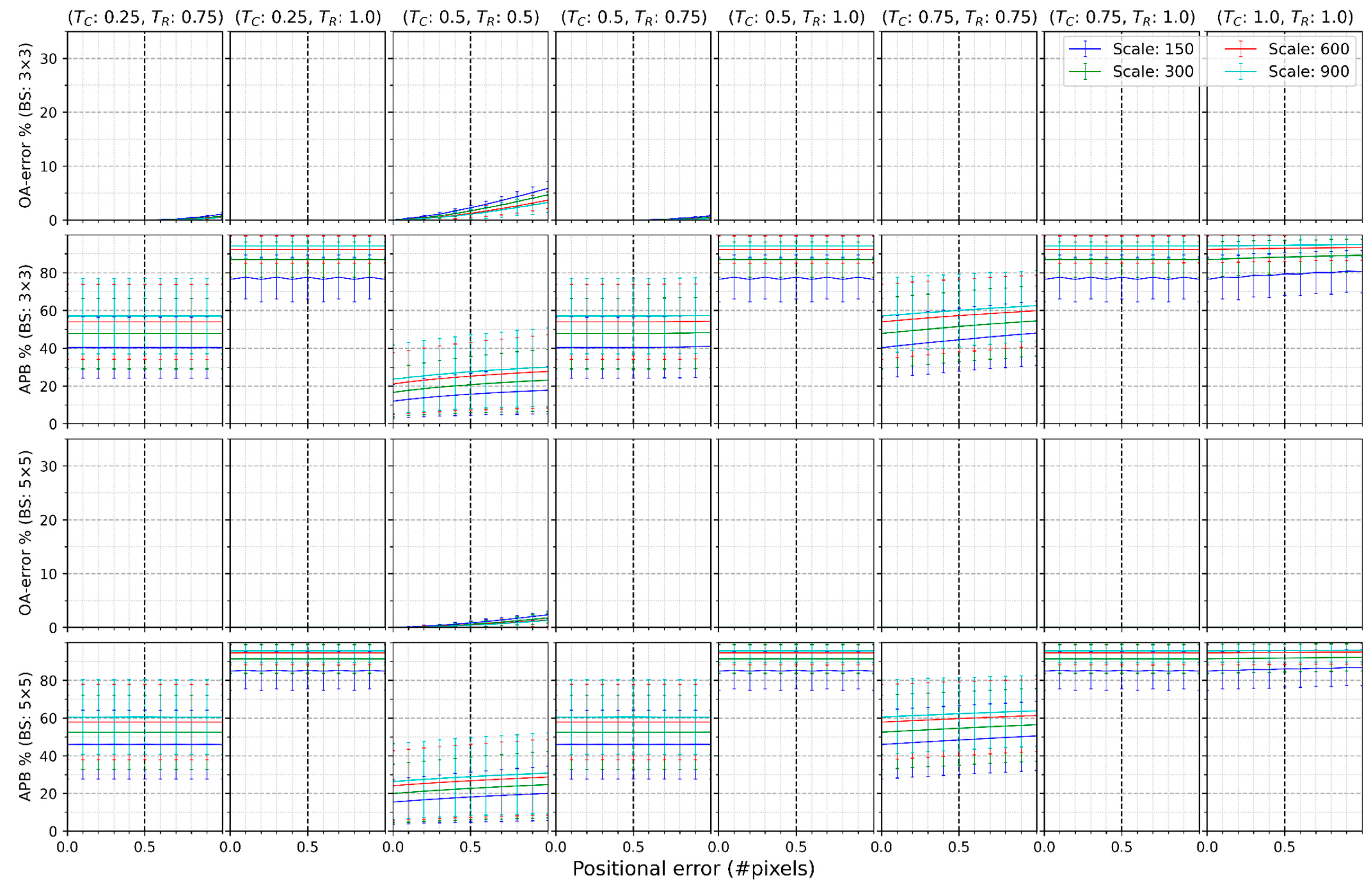
Figure 3 shows the mean and standard deviation of and for the twelve study sites at the four spatial scales when the classification map consisted of seven classes (Level I) using a block size of 3 × 3 or 5 × 5 pixels. Figure 3 was divided into 60 sub-figures composed of four rows and 15 columns. The entire figure could not fit on one page and, therefore, was split into two pages by columns. The first two rows show the results of applying a block size of 3 × 3 pixels, while the last two rows display the results of the block size of 5 × 5 pixels. Each column presents the outcome of a pair of (). There should have been 25 combinations (columns) of (). However, for example, () generated almost the same results as () because, in this research, the classification map and its reference data were both generated from NLCD 2015. Therefore, only results of when were shown. Each line in a sub-figure represents a scale.
In the sub-figure () of the first row of Figure 3, the mean value of grows as the positional error increases, and so does the standard deviation of . For example, the mean and standard deviation of were 5.08% and 1.53 at a positional error of 0.5 pixels when the scale was 150 m. The two values became 9.59% and 2.88 when the positional error reached 1 pixel.
As shown in the first row of sub-figures in Figure 3, the exhibited similar values when both and were no more than 0.25. As either or grew, dropped. There was a significant reduction in if either or attained 0.5. Almost no positional effect existed when either threshold achieved 0.75 or over. In addition, the mean values of at various scales were very close regardless of the labeling threshold.
The second row of sub-figures in Figure 3 reflects under multiple choices of (). was less than 0.2% when either or was no greater than 0.25. As either or increased, increased. When , the average varied between 5.84% and 11.63% and the standard deviation fluctuated between 3.18% and 6.36%. When or reached 0.75, the average ranged from 30.81% to 46.73%. The average varied from 72.09% to 94.11% when either or reached 1.0. Most mean values of were relatively stable regardless of the positional errors, but when (, ) was either (0.5, 0.5) or (0.75, 0.75), the average lines displayed an increasing trend. Finally, a higher spatial scale (e.g., 150 m) generated lower regardless of or .
The third and fourth rows of sub-figures of Figure 3 present and respectively, using a block size of 5 × 5 pixels. Compared to the results in the block size of 3 × 3 pixels, a greater block size further reduced the positional effect but slightly increased compared with the 3 × 3 pixel block.
The results presented in Figure 3 are also reflected in Figure 4. However, the classification scheme used in Figure 4 shows the results of the Level II (12 classes) analysis. The classification scheme with 12 classes presented higher and compared with seven-classes results shown in Figure 3.
Figure 5 presents the mean and standard deviation of and at the four scales for each study site when the classification scheme consisted of seven classes (Level I). Each curve represents a study site in each sub-figure.
The upper-left sub-figure of Figure 5 describes the resulting from positional errors ranging from 0 to 1.0 pixels when both and equal 0. The highest approximated 7.87 ± 0.50% and 14.41 ± 1.11% at the positional error of 0.5 and 1.0 pixels, respectively, for study site 12. A study site with a smaller LSI caused a lower positional effect than one with a larger LSI. For example, the line of study site #3 with an LSI of 377.4 was below the line of study site #4 with an LSI of 439.9. However, this did not hold for all study sites. For instance, study site #11 with an LSI of 465.2 was below study site 2 with an LSI of 353.7.
No significant difference in was observed when neither threshold surpassed 0.25. decreased as either or increased from 0.5 to 1.0. For example, there was almost no positional effect when either threshold exceeded 0.75.
The second row of sub-figures in Figure 5 reflects the of each study site under multiple choices of (). The values of average approximated 0 if neither nor was over 0.25. lines were, on average, between 19.92% and 3.03%, between 25.39% and 63.50%, and between 71.13% and 96.08% when either threshold reached 0.5, 0.75, and 1.0, respectively.
Compared to the first two rows of Figure 5, using a block size of 5 × 5 pixels further decreased the positional effect but slightly increased the versus the results of 3 × 3 pixels (see rows 3 and 4). For example, all study sites’ lines were under 5% at the positional errors of 0.5 when using 5 × 5 pixel blocks, while most were above 5% using 3 × 3 pixels.
The patterns found in Figure 6 are similar to that of Figure 5. The only difference is that each line in Figure 6 is higher than the corresponding one in Figure 5 because the classification scheme consists of more classes (12 instead of seven).
Most remote-sensing applications reported that a half-pixel registration was achieved. Therefore, within each sub-figure, a vertical line marking 0.5 pixels was emphasized. Figure 3 shows that the was 5.08 ± 1.52% if neither nor was more significant than 0.25 using 3 × 3 pixel blocks. The reduced to under 5% if either threshold reached 0.5, but the varied between 5.88 ± 3.2% (results of the scale of 150) and 11.62 ± 6.29% (results of the scale 900). There was nearly no positional effect when either threshold reached or exceeded 0.75, but the was between 30.01% and 46.68% and over 60%, respectively. Using 5 × 5 pixel blocks slightly reduced but increased the . For example, the was 3.23 ± 0.99% when (, ) was equal to (0, 0.25). Figure 5 displays that of most study sites was below 5%, except study sites 4, 5, 9, 10, and 12 when both and were less than 0.25. The of all study sites was under 5%, and they abandoned 3.01 ± 0.93% to 19.87 ± 5.43% if any threshold reached 0.5. approximated 0, but varied between 25.39% and 63.51% and over 755.88% if the threshold attained 0.75 and 1.0, respectively. The results in Figure 4 and Figure 6 show more but also an increase in because of more classes, and the trend is the same in Figure 3 and Figure 5.
5. Discussion
Land-cover maps derived from remote-sensing classification contain classification errors because of the uncertainties such as imperfect training data or classification algorithms [51,52]. These maps were validated by thematic accuracy assessment and then presented as error matrices [53]. Unfortunately, the validation itself includes uncertainties that also affect the thematic accuracies. Choosing the assessment units is one of the sources of uncertainty. Pixels, blocks, or polygons are three options of assessment units [34]. This research focused on a block-based accuracy assessment for validating per-pixel classification. The analysis was performed to evaluate the impact of positional errors on thematic accuracy assessment when using a block of pixels with varying labeling rules as the assessment unit. This study aimed to answer the following questions. First, what is the remaining positional effect utilizing a block as the assessment unit combined with multiple labeling rules? Second, how do these results differ when altering the spatial pattern of landscape, the classification scheme, and the spatial scale of classification map? The results were examined in terms of and .
The results showed that the labeling threshold had a significant impact on the and . The effect depends on the highest value between (Figure 3: () vs. ()). As a result, we defined a to explain the effect of the labeling threshold. If reaches 0.75 or 1.0, almost disappears. Still, exceeded 25% and 60%, respectively, across all the figures, which implies that many blocks were abandoned from the sampling population. This abandonment of samples offers another set of issues that must be considered when conducting a remote-sensing accuracy assessment. In addition, there was no significant difference in if was no more than 0.25 because, within a 3 × 3 or 5 × 5 pixel block, the minimum percentage of the majority class was 22.2% or 16% for the classification scheme consisting of seven classes. The minimum proportion became 11.1% or 12% for the classification scheme comprised of 12 categories. There is a rare chance that classes within a block are randomly selected from the classification scheme. Therefore, the following analysis focused on in two groups: and . For convenience, we also defined a symbol like to indicate the remaining when a block-based validation was performed where the block size was 3 × 3 pixels, was 0.25, and the positional error was 0.5 pixels. The same idea was applied to .
During remote-sensing accuracy assessment, the source of positional error derives from the geo-registration of the remote sensing images and the GPS error, if the reference is collected from a field survey [54]. Most land cover projects reported the thematic and positional accuracy together [55,56,57]. The positional errors of IGBP, UMD, GLC 2000, MCD12, GLCNMO, and GlobCover are 1 pixel, 1 pixel, 0.3–0.47 pixels, 0.1–0.2 pixels, 0.19–0.69 pixels, and 0.26 pixels relative to their spatial resolutions of 1000 m, 1000 m, 1000 m, 500 m, 1000/500 m, and 300 m, respectively (Table 7 of Ref. [26]). Using single-pixel as an assessment unit created 31.92%, 31.92%, and 15.06%–18.92%, 5.50%–10.41%, 10.41%–27.37% and 13.56% of [26]. If utilizing positional error, spatial resolution, and classification scheme of these global land-cover datasets and comparing their results to the best match the results of our research (Figure 4 and Figure 6), the remaining positional effect in block-based accuracy assessment is shown in Figure 7. The average was 12.22%, 12.22%, 4.25% to 6.73%, 1.46% to 2.89%, 2.89% to 9.08%, and 4.28%. This implies that using 3 × 3 pixel blocks with effectively reduced the positional effect but the remaining in IGBP or UMD was still above 10%. Utilizing of 0.5 would decrease all under 10%, but remove 16.62 ± 12.90% to 23.56 ± 18.21% of blocks from the sampling populations. The high variance was derived from the varied landscape characteristics among study sites (Figure 6), which means that for IGBP or UMD, the strategy highly depends on the spatial characteristics. If limiting under 10%, then the LSI should be less than 377.4 to apply of 0.5. If the were widened to under 20%, then the LSI should be beneath 483.2. Employing a block size of 5 × 5 pixels may be another option, but for global land-cover mapping using MODIS at the scale of 1 km, determining whether sampling 5 × 5 km is practical or not needs further research. This research highly suggests the global land-cover mapping derived from medium-resolution images (150 m to 1 km) take 3 × 3 pixels as an assessment unit into account for validation.
The results also showed that caused by a half-pixel positional error was 5.08 ± 1.52% and 6.91 ± 3.19%, respectively, for classification schemes of 7 and 12 classes. This is a significant reduction compared with the range from 12.05% to 17.97% of reported by Gu and Congalton [26] using a single-pixel as an assessment unit. This indicates that for most classification applications with less than 12 classes, 3 × 3 pixel blocks with a simple majority rule would result in under 10%.
Collecting reference samples is very expensive in remote-sensing accuracy assessment. On the one hand, we want to make sure the resultant accuracy measures are reliable, minimizing the positional effect. On the other hand, we require the implementation to be practical, minimizing the labor in the field. Using 5 × 5 pixels could further reduce positional errors by an average of about 2%. However, increasing the size of the sample block may increase the amount of effort required to collect the reference data in the field.
This paper found that the larger the number of map classes and the more heterogeneous the landscape characteristics, the greater the , which is consistent with previous research [26]. The underlying reason is that either of these factors (higher number of map classes and more heterogeneous landscape) generates a higher possibility that a block may be moved to a position incorporating other classes that alter the label of this block. This research also discovered that a study site with a larger LSI does not always produce a higher positional effect. LSI is incomplete in that it only calculates the total length of edge normalized by the minimum total length of edge within a landscape without considering the contagion index [58]. Future research could explore which landscape indexes are best to analyze the positional effect. Across all sub-figures presented here, the average lines caused by spatial scale (Figure 3 and Figure 4) approximated each other, but a coarser scale abandoned more blocks from the sampling population. This abandonment results from the fact that a larger block has a higher possibility of heterogeneous labels.
This research was a controlled experiment where the thematic errors in the error matrix were caused by the positional errors only, which is distinct from previous studies that included classification error or sampling error while analyzing the positional effect [28,33,34]. Combining multiple sources of errors would make the results difficult to explain. However, this research also has several limitations. First, this study covered the spatial scales ranging from 150 m to 900 m. As the spatial resolution of the image grew higher, especially the images acquired from unmanned aerial vehicles (UAV) [59], the positional error in these images was much greater than 1 pixel because of GPS error or the absence of a high-precision digital-elevation model (DEM) [60]. What labeling threshold can be used to remove the remains unknown. However, for high-resolution image classification, a segmentation is usually performed beforehand [61]. What relationship exists between object size and positional error needs further research. Second, this research comprises two classification schemes with only 7 and 12 classes. This is limited by the classification scheme of NLCD 2015. Third, this research proved that block-based assessment is more reliable than single-pixel-based accuracy assessment from the viewpoint of positional errors. This creates further research for other block-based accuracy assessment. For example, how to effectively sample the blocks becomes essential. Previous research has shown that stratified sampling was preferred over simple random and systematic sampling [16]. What kind of information such as the block’s categorical label, proportion, or structure is more effective to stratify the sampling population is also crucial. Finally, when assessing the accuracy of a map using a block of pixels to compensate for positional error, the original map is modified by the thresholds and labeling rules used to determine the sample label. There is a trade-off here between using a block to assess the thematic accuracy of a modified map or using a single pixel to assess the original map while incorporating substantial positional error into the thematic accuracy. This paper, in combination with Gu and Congalton [26], presented the advantages and limitations of using each approach. The next step in this analysis needing further research is the comparison of the original pixel maps with the maps assessed here that resulted from the thresholds and labeling rules selected. This analysis would produce metadata demonstrating the difference between the realized thematic map and the “hypothetical” map produced using the thresholds for labeling the blocks. The magnitude of differences here would be highly dependent on whether a minimum mapping unit was selected for the original mapping project that was larger than a single pixel or if the single pixel classification map was retained. The user of the map could then decide whether to use a single pixel for the assessment unit and retain all the thematic error caused by positional error or to use a block of pixels for the assessment unit to compensate for positional error, but understand that the map being assessed is not the original pixel map. The results presented here are a compilation of 52,800 error matrices (12 study sites × 4 scales × 2 classification schemes × 2 block sizes × 11 positional errors × 25 thresholds = 52,800) and such a comparison was beyond the scope of this paper.
6. Conclusions
Choosing the assessment unit is a critical step in the thematic accuracy assessment of remote-sensing classification. This research focused on analyzing blocks as assessment units for validating per-pixel classification using medium-spatial-resolution images. The study was based on the uncertainties caused by positional errors. Block size, labeling threshold, landscape characteristics, classification scheme, and spatial scales were regarded as factors to impact the choice of blocks as the assessment unit. This research has the following conclusions:
- (1)
- Labeling thresholds greater or equal to 0.75 are not a good choice for determining a block’s label. A labeling threshold equal to 0.5 applies to a higher spatial scale with lower heterogeneity. A labeling threshold less than 0.25 is appropriate for most remote sensing applications.
- (2)
- Blocks with the size of 5 × 5 pixels remove, on average, around 2% more positional error compared with a 3 × 3 pixel block. However, it may not be practical to collect reference samples of this size if the reference data are collected by field survey.
- (3)
- The in most land cover mapping projects except IGBP and UMD can be reduced to under 10% if using 3 × 3 pixel blocks with the labeling threshold being less than 0.25.
- (4)
- The in most remote-sensing applications achieving half-pixel registration is under 10% if using a 3 × 3 pixel block with labeling threshold being less than 0.25.
- (5)
- More chasses in a classification scheme or higher heterogeneity increase the positional effect.
- (6)
- Further research can focus on how to sample blocks based on the proportion or structure of the blocks.
Author Contributions
J.G. and R.G.C. conceived and designed the experiments. J.G. performed the experiments and analyzed the data with guidance from R.G.C.; J.G. wrote the paper. R.G.C. edited and finalized the paper and manuscript. All authors have read and agreed to the published version of the manuscript.
Funding
Partial funding was provided by the New Hampshire Agricultural Experiment Station. This is Scientific Contribution Number: #2909. This work was supported by the USDA National Institute of Food and Agriculture McIntire Stennis Project #NH00095-M (Accession #1015520).
Conflicts of Interest
The authors declare no conflict of interest.
References
- Wulder, M.A.; Coops, N.C.; Roy, D.P.; White, J.C.; Hermosilla, T. Land cover 2.0. Int. J. Remote Sens. 2018, 39, 4254–4284. [Google Scholar] [CrossRef] [Green Version]
- Estes, L.; Chen, P.; Debats, S.; Evans, T.; Ferreira, S.; Kuemmerle, T.; Ragazzo, G.; Sheffield, J.; Wolf, A.; Wood, E.; et al. A large-area, spatially continuous assessment of land cover map error and its impact on downstream analyses. Glob. Chang. Biol. 2018, 24, 322–337. [Google Scholar] [CrossRef] [Green Version]
- Wang, C.; Wang, Y.; Wang, R.; Zheng, P. Modeling and evaluating land-use/land-cover change for urban planning and sustainability: A case study of Dongying city, China. J. Clean. Prod. 2018, 172, 1529–1534. [Google Scholar] [CrossRef]
- Zaldo-Aubanell, Q.; Serra, I.; Sardanyés, J.; Alsedà, L.; Maneja, R. Reviewing the reliability of Land Use and Land Cover data in studies relating human health to the environment. Environ. Res. 2021, 194, 110578. [Google Scholar] [CrossRef]
- Bartholomé, E.; Belward, A.S. GLC2000: A new approach to global land cover mapping from Earth observation data. Int. J. Remote Sens. 2005, 26, 1959–1977. [Google Scholar] [CrossRef]
- Sulla-Menashe, D.; Gray, J.; Abercrombie, S.P.; Friedl, M.A. Hierarchical mapping of annual global land cover 2001 to present: The MODIS Collection 6 Land Cover product. Remote Sens. Environ. 2019, 222, 183–194. [Google Scholar] [CrossRef]
- Chen, J.; Chen, J.; Liao, A.; Cao, X.; Chen, L.; Chen, X.; He, C.; Han, G.; Peng, S.; Lu, M.; et al. Global land cover mapping at 30m resolution: A POK-based operational approach. ISPRS J. Photogramm. Remote Sens. 2015, 103, 7–27. [Google Scholar] [CrossRef] [Green Version]
- Congalton, R.G.; Green, K. Assessing the Accuracy of Remotely Sensed Data: Principles and Practices; CRC: Boca Raton, FL, USA, 2019. [Google Scholar]
- Sylvander, S.; Henry, P.; Bastin-thiry, C.; Meunier, F.; Fuster, D. VEGETATION geometrical image quality. Bull. de la Société Française de Photogrammétrie et de Télédétection 2000, 159, 59–65. [Google Scholar]
- Congalton, R.G. A review of assessing the accuracy of classifications of remotely sensed data. Remote Sens. Environ. 1991, 37, 35–46. [Google Scholar] [CrossRef]
- Stehman, S.V. Sampling designs for accuracy assessment of land cover. Int. J. Remote Sens. 2009, 30, 5243–5272. [Google Scholar] [CrossRef]
- Olofsson, P.; Foody, G.M.; Herold, M.; Stehman, S.V.; Woodcock, C.E.; Wulder, M.A. Good practices for estimating area and assessing accuracy of land change. Remote Sens. Environ. 2014, 148, 42–57. [Google Scholar] [CrossRef]
- Congalton, R.; Oderwald, R.G.; Mead, R. Assessing Landsat classification accuracy using discrete multivariate analysis statistical techniques. Photogramm. Eng. Remote Sens. 1983, 49, 1671–1678. [Google Scholar]
- Foody, G.M. Status of land cover classification accuracy assessment. Remote Sens. Environ. 2002, 80, 185–201. [Google Scholar] [CrossRef]
- Stehman, S.V.; Czaplewski, R.L. Design and Analysis for Thematic Map Accuracy Assessment: Fundamental Principles. Remote Sens. Environ. 1998, 64, 331–344. [Google Scholar] [CrossRef]
- Stehman, S.V.; Foody, G.M. Key issues in rigorous accuracy assessment of land cover products. Remote Sens. Environ. 2019, 231, 111199. [Google Scholar] [CrossRef]
- Foody, G.M. Assessing the accuracy of land cover change with imperfect ground reference data. Remote Sens. Environ. 2010, 114, 2271–2285. [Google Scholar] [CrossRef] [Green Version]
- Congalton, R.G. Thematic and positional accuracy assessment of digital remotely sensed data. In Proceedings of the 7th Annual Forest Inventory and Analysis Symposium, Portland, ME, USA, 3–6 October 2005. [Google Scholar]
- Stehman, S.V. Sampling Designs for Assessing Map Accuracy. In Proceedings of the 8th International Symposium on Spatial Accuracy Assessment in Natural Resources and Environmental Sciences, Shanghai, China, 25–27 June 2008. [Google Scholar]
- Giri, C.; Pengra, B.; Long, J.; Loveland, T. Next generation of global land cover characterization, mapping, and monitoring. Int. J. Appl. Earth Obs. Geoinf. 2013, 25, 30–37. [Google Scholar] [CrossRef]
- Belgiu, M.; Drăguţ, L. Random forest in remote sensing: A review of applications and future directions. ISPRS J. Photogramm. Remote Sens. 2016, 114, 24–31. [Google Scholar] [CrossRef]
- Mountrakis, G.; Im, J.; Ogole, C. Support vector machines in remote sensing: A review. ISPRS J. Photogramm. Remote Sens. 2011, 66, 247–259. [Google Scholar] [CrossRef]
- Janssen, L.L.F.; Vanderwel, F.J.M. Accuracy assessment of satellite-derived land-cover data-a review. Photogramm. Eng. Remote Sens. 1994, 60, 419–426. [Google Scholar]
- Richards, J.A. Classifier performance and map accuracy. Remote Sens. Environ. 1996, 57, 161–166. [Google Scholar] [CrossRef]
- Morales-Barquero, L.; Lyons, M.B.; Phinn, S.R.; Roelfsema, C.M. Trends in Remote Sensing Accuracy Assessment Approaches in the Context of Natural Resources. Remote Sens. 2019, 11, 2305. [Google Scholar] [CrossRef] [Green Version]
- Gu, J.; Congalton, R. Analysis of the Impact of Positional Accuracy When Using a Single Pixel for Thematic Accuracy Assessment. Remote Sens. 2020, 12, 4093. [Google Scholar] [CrossRef]
- Gu, J.; Congalton, R.G.; Pan, Y. The Impact of Positional Errors on Soft Classification Accuracy Assessment: A Simulation Analysis. Remote Sens. 2015, 7, 579–599. [Google Scholar] [CrossRef] [Green Version]
- Powell, R.; Matzke, N.; de Souza, C.; Clark, M.; Numata, I.; Hess, L.; Roberts, D. Sources of error in accuracy assessment of thematic land-cover maps in the Brazilian Amazon. Remote Sens. Environ. 2004, 90, 221–234. [Google Scholar] [CrossRef]
- Brown, K.M.; Foody, G.M.; Atkinson, P.M. Modelling geometric and misregistration error in airborne sensor data to enhance change detection. Int. J. Remote Sens. 2007, 28, 2857–2879. [Google Scholar] [CrossRef]
- Yang, K.; Pan, A.; Yang, Y.; Zhang, S.; Ong, S.H.; Tang, H. Remote Sensing Image Registration Using Multiple Image Features. Remote Sens. 2017, 9, 581. [Google Scholar] [CrossRef] [Green Version]
- Yang, Z.; Dan, T.; Yang, Y. Multi-Temporal Remote Sensing Image Registration Using Deep Convolutional Features. IEEE Access 2018, 6, 38544–38555. [Google Scholar] [CrossRef]
- Beekhuizen, J.; Heuvelink, G.B.M.; Biesemans, J.; Reusen, I. Effect of DEM Uncertainty on the Positional Accuracy of Airborne Imagery. IEEE Trans. Geosci. Remote Sens. 2010, 49, 1567–1577. [Google Scholar] [CrossRef]
- Plourde, L.; Congalton, R.G. Sampling method and sample placement: How do they affect the accuracy of remotely sensed maps? Photogramm. Eng. Remote Sens. 2003, 69, 289–297. [Google Scholar] [CrossRef]
- Stehman, S.V.; Wickham, J.D. Pixels, blocks of pixels, and polygons: Choosing a spatial unit for thematic accuracy assessment. Remote Sens. Environ. 2011, 115, 3044–3055. [Google Scholar] [CrossRef]
- Carmel, Y. Controlling Data Uncertainty via Aggregation in Remotely Sensed Data. IEEE Geosci. Remote Sens. Lett. 2004, 1, 39–41. [Google Scholar] [CrossRef]
- Carmel, Y. Aggregation as a Means of Increasing Thematic Map Accuracy. In GeoDynamics; CRC Press: Boca Raton, FL, USA, 2004; pp. 29–38. [Google Scholar]
- Clinton, N.; Holt, A.; Scarborough, J.; Yan, L.; Gong, P. Accuracy Assessment Measures for Object-based Image Segmentation Goodness. Photogramm. Eng. Remote Sens. 2010, 76, 289–299. [Google Scholar] [CrossRef]
- Ye, S.; Pontius, R.G.; Rakshit, R. A review of accuracy assessment for object-based image analysis: From per-pixel to per-polygon approaches. ISPRS J. Photogramm. Remote Sens. 2018, 141, 137–147. [Google Scholar] [CrossRef]
- Huang, Z.; Lees, B. Assessing a single classification accuracy measure to deal with the imprecision of location and class: Fuzzy weighted kappa versus kappa. J. Spat. Sci. 2007, 52, 1–12. [Google Scholar] [CrossRef]
- Latifovic, R.; Olthof, I. Accuracy assessment using sub-pixel fractional error matrices of global land cover products derived from satellite data. Remote Sens. Environ. 2004, 90, 153–165. [Google Scholar] [CrossRef]
- Yadav, K.; Congalton, R.G. Issues with Large Area Thematic Accuracy Assessment for Mapping Cropland Extent: A Tale of Three Continents. Remote Sens. 2017, 10, 53. [Google Scholar] [CrossRef] [Green Version]
- Hammond, T.O.; Verbyla, D.L. Optimistic bias in classification accuracy assessment. Int. J. Remote Sens. 1996, 17, 1261–1266. [Google Scholar] [CrossRef]
- Dai, X.; Khorram, S. The effects of image misregistration on the accuracy of remotely sensed change detection. IEEE Trans. Geosci. Remote Sens. 1998, 36, 1566–1577. [Google Scholar] [CrossRef] [Green Version]
- Chen, G.; Zhao, K.; Powers, R. Assessment of the image misregistration effects on object-based change detection. ISPRS J. Photogramm. Remote Sens. 2014, 87, 19–27. [Google Scholar] [CrossRef]
- Gerçek, D.; Cesmeci, D.; Gullu, M.K.; Erturk, A.; Erturk, S. An automated fine registration of multisensor remote sensing imagery. 2012 IEEE Int. Geosci. Remote Sens. Symp. 2012, 1361–1364. [Google Scholar] [CrossRef]
- Dong, Y.; Long, T.; Jiao, W.; He, G.; Zhang, Z. A Novel Image Registration Method Based on Phase Correlation Using Low-Rank Matrix Factorization With Mixture of Gaussian. IEEE Trans. Geosci. Remote Sens. 2018, 56, 446–460. [Google Scholar] [CrossRef]
- Foody, G.M. Explaining the unsuitability of the kappa coefficient in the assessment and comparison of the accuracy of thematic maps obtained by image classification. Remote Sens. Environ. 2020, 239, 111630. [Google Scholar] [CrossRef]
- Warrens, M.J. Properties of the quantity disagreement and the allocation disagreement. Int. J. Remote Sens. 2015, 36, 1439–1446. [Google Scholar] [CrossRef]
- Pontius, R.G., Jr.; Millones, M. Death to Kappa: Birth of quantity disagreement and allocation disagreement for accuracy assessment. Int. J. Remote Sens. 2011, 32, 4407–4429. [Google Scholar] [CrossRef]
- McGarigal, K.; Marks, B.J. FRAGSTATS: Spatial Pattern Analysis Program for Quantifying Landscape Structure; General Technical Reports; Department of Agriculture, Forest Service, Pacific Northwest Research Station: Portland, OR, USA, 1995; Volume 122, p. 351.
- Congalton, R.G.; Gu, J.; Yadav, K.; Thenkabail, P.; Ozdogan, M. Global Land Cover Mapping: A Review and Uncertainty Analysis. Remote Sens. 2014, 6, 12070–12093. [Google Scholar] [CrossRef] [Green Version]
- Steffen, F.; Linda, S.; Ian, M.; Christian, S.; Michael, O.; Marijn van der, V.; Hannes, B.; Petr, H.; Frédéric, A. Highlighting continued uncertainty in global land cover maps for the user community. Environ. Res. Lett. 2011, 6, 044005. [Google Scholar]
- Gu, J.; Congalton, R.G. The Positional Effect in Soft Classification Accuracy Assessment. Am. J. Remote Sens. 2019, 7, 50. [Google Scholar] [CrossRef]
- McRoberts, R.E. The effects of rectification and Global Positioning System errors on satellite image-based estimates of forest area. Remote Sens. Environ. 2010, 114, 1710–1717. [Google Scholar] [CrossRef]
- Brovelli, M.A.; Molinari, M.E.; Hussein, E.; Chen, J.; Li, R. The First Comprehensive Accuracy Assessment of GlobeLand30 at a National Level: Methodology and Results. Remote Sens. 2015, 7, 4191–4212. [Google Scholar] [CrossRef] [Green Version]
- Bicheron, P.; Amberg, V.; Bourg, L.; Petit, D.; Huc, M.; Miras, B.; Brockmann, C.; Hagolle, O.; Delwart, S.; Ranera, F.; et al. Geolocation Assessment of MERIS GlobCover Orthorectified Products. IEEE Trans. Geosci. Remote Sens. 2011, 49, 2972–2982. [Google Scholar] [CrossRef]
- Sylvander, S.; Albert-Grousset, I.; Henry, P. Geometrical performance of the VEGETATION products. In Proceedings of the IGARSS 2003, 2003 IEEE International Geoscience and Remote Sensing Symposium, Proceedings (IEEE Cat. No.03CH37477), Toulouse, France, 21–25 July 2004; Institute of Electrical and Electronics Engineers (IEEE): Toulouse, France, 2004; Volume 571, pp. 573–575. [Google Scholar]
- Evelin, U.; Marc, A.A.; Jüri, R.; Riho, M.; Ülo, M. Landscape Metrics and Indices: An Overview of Their Use in Landscape Research. Living Rev. Landsc. Res. 2009, 5–14. [Google Scholar] [CrossRef]
- Zhang, J.; Hu, J.; Lian, J.; Fan, Z.; Ouyang, X.; Ye, W. Seeing the forest from drones: Testing the potential of lightweight drones as a tool for long-term forest monitoring. Biol. Conserv. 2016, 198, 60–69. [Google Scholar] [CrossRef]
- Ren, X.; Sun, M.; Jiang, C.; Liu, L.; Huang, W. An Augmented Reality Geo-Registration Method for Ground Target Localization from a Low-Cost UAV Platform. Sensors 2018, 18, 3739. [Google Scholar] [CrossRef] [PubMed] [Green Version]
- Hossain, M.D.; Chen, D. Segmentation for Object-Based Image Analysis (OBIA): A review of algorithms and challenges from remote sensing perspective. ISPRS J. Photogramm. Remote Sens. 2019, 150, 115–134. [Google Scholar] [CrossRef]
Figure 1.
An example of using 3 × 3 pixel blocks as assessment units to validate the classification map where the positional error is 1 pixel. In this case, the classification map has three classes: non-vegetation, vegetation, and water. The majority rule with 4 combinations of labeling thresholds () were applied to each block to determine its label. As the labeling threshold gets higher, more blocks were abandoned (Null).

Figure 2.
Locations of twelve study sites.

Figure 3.
Mean and standard deviation of and of twelve study sites at different scales when the classification consists of seven classes using a block size of 3 × 3 or 5 × 5 pixels.
Figure 3.
Mean and standard deviation of and of twelve study sites at different scales when the classification consists of seven classes using a block size of 3 × 3 or 5 × 5 pixels.


Figure 4.
Mean and standard deviation of and of twelve study sites at different scales when the classification consists of 12 classes using a block size of 3 × 3 or 5 × 5 pixels.
Figure 4.
Mean and standard deviation of and of twelve study sites at different scales when the classification consists of 12 classes using a block size of 3 × 3 or 5 × 5 pixels.


Figure 5.
Mean and standard deviation of and of four spatial scales at different study sites where the classification scheme consists of seven classes using block size of 3 × 3 or 5 × 5 pixels.
Figure 5.
Mean and standard deviation of and of four spatial scales at different study sites where the classification scheme consists of seven classes using block size of 3 × 3 or 5 × 5 pixels.


Figure 6.
Mean and standard deviation of and of four spatial scales at different study sites where the classification scheme consists of 12 classes using a block size of 3 × 3 or 5 × 5 pixels.
Figure 6.
Mean and standard deviation of and of four spatial scales at different study sites where the classification scheme consists of 12 classes using a block size of 3 × 3 or 5 × 5 pixels.


Figure 7.
The remaining and in block-based validation of global land-cover datasets according to their spatial resolution, classification scheme, and positional errors.
Figure 7.
The remaining and in block-based validation of global land-cover datasets according to their spatial resolution, classification scheme, and positional errors.


Table 1.
Error matrix for thematic accuracy assessment.
| Reference | |||||||
|---|---|---|---|---|---|---|---|
| Class 1 | Class 2 | … | Class C | Sample Total | Population Total | ||
| Classification | Class 1 | n11 | n12 | … | n1C | n1+ | N1 |
| Class 2 | n21 | n22 | … | n2C | n2+ | N2 | |
| … | … | … | … | … | … | … | |
| Class C | nC1 | nC2 | … | nCC | nC+ | NC | |
| n+1 | n+2 | … | n+C | n | N | ||
| Accuracy measures | |||||||
Table 2.
Two levels of the classification scheme creating from the original NLCD 2015 classification scheme.
Table 2.
Two levels of the classification scheme creating from the original NLCD 2015 classification scheme.
| Level I | Class Name | Level II | Class Name | Original Level | Original Classification Scheme |
|---|---|---|---|---|---|
| 1 | Forest | 1 | Needleleaf | 1 | Temperate or sub-polar needleleaf forest |
| 2 | Sub-polar taiga needleleaf forest | ||||
| 2 | Broadleaf | 3 | Tropical or sub-tropical broadleaf evergreen forest | ||
| 4 | Tropical or sub-tropical broadleaf deciduous forest | ||||
| 5 | Temperate or sub-polar broadleaf deciduous forest | ||||
| 3 | Mixed | 6 | Mixed forest | ||
| 2 | Shrub | 4 | Shrub | 7 | Tropical or sub-tropical shrubland |
| 8 | Temperate or sub-polar shrubland | ||||
| 3 | Herbaceous | 5 | Grassland | 9 | Tropical or sub-tropical grassland |
| 10 | Temperate or sub-polar grassland | ||||
| 6 | Lichen-moss | 11 | Sub-polar or polar shrubland-lichen-moss | ||
| 12 | Sub-polar or polar grassland-lichen-moss | ||||
| 13 | Sub-polar or polar barren-lichen-moss | ||||
| 4 | Wetland | 7 | Wetland | 14 | Wetland |
| 5 | Cropland | 8 | Cropland | 15 | Cropland |
| 6 | Urban/Bare | 9 | Barren lands | 16 | Barren lands |
| 10 | Urban | 17 | Urban | ||
| 7 | Water | 11 | Water | 18 | Water |
| 0 | Background (Ocean) | ||||
| 12 | Snow and Ice | 19 | Snow and Ice |
Table 3.
Landscape shape index (LSI) values of the twelve study sites.
| Level | Landscape Shape Index (LSI) | |||||||||||
|---|---|---|---|---|---|---|---|---|---|---|---|---|
| Site #1 | Site #2 | Site #3 | Site #4 | Site #5 | Site #6 | Site #7 | Site #8 | Site #9 | Site #10 | Site #11 | Site #12 | |
| I | 302.0 | 353.7 | 377.4 | 439.9 | 461.7 | 456.0 | 483.2 | 352.2 | 508.9 | 589.4 | 465.2 | 685.8 |
| II | 310.3 | 365.9 | 393.5 | 448.0 | 465.2 | 485.8 | 557.6 | 650.1 | 688.3 | 707.3 | 860.7 | 938.1 |
Publisher’s Note: MDPI stays neutral with regard to jurisdictional claims in published maps and institutional affiliations. |
© 2021 by the authors. Licensee MDPI, Basel, Switzerland. This article is an open access article distributed under the terms and conditions of the Creative Commons Attribution (CC BY) license (https://creativecommons.org/licenses/by/4.0/).
Share and Cite
MDPI and ACS Style
Gu, J.; Congalton, R.G. Analysis of the Impact of Positional Accuracy When Using a Block of Pixels for Thematic Accuracy Assessment. Geographies 2021, 1, 143-165. https://0-doi-org.brum.beds.ac.uk/10.3390/geographies1020009
AMA Style
Gu J, Congalton RG. Analysis of the Impact of Positional Accuracy When Using a Block of Pixels for Thematic Accuracy Assessment. Geographies. 2021; 1(2):143-165. https://0-doi-org.brum.beds.ac.uk/10.3390/geographies1020009
Chicago/Turabian StyleGu, Jianyu, and Russell G. Congalton. 2021. "Analysis of the Impact of Positional Accuracy When Using a Block of Pixels for Thematic Accuracy Assessment" Geographies 1, no. 2: 143-165. https://0-doi-org.brum.beds.ac.uk/10.3390/geographies1020009