Article

The Importance of Connected and Interspersed Urban Green and Blue Space for Biodiversity: A Case Study in Cork City, Ireland

1
Department of Geography, University College Cork, T12 K8AF Cork, Ireland
2
Environmental Research Institute, University College Cork, T23 XE10 Cork, Ireland
*
Author to whom correspondence should be addressed.
Submission received: 2 June 2021 / Revised: 30 September 2021 / Accepted: 22 October 2021 / Published: 2 November 2021
(This article belongs to the Special Issue Feature Papers of Geographies in 2021)

Abstract

:
Urban green and blue space (UGBS) is becoming increasingly important for supporting biodiversity, with the spatial configuration of these landscapes essential to supporting a range of taxa. The role of UGBS for supporting biodiversity is well established, but there remains a lack of consensus on the importance of the overall landscape configuration and the scale at which these configurations are analyzed. Moreover, statistical models are often compounded by coarse representations of UGBS that ignore ‘invisible’ spaces (i.e., gardens and brownfield sites). Using Sentinel-2 satellite data and a maximum likelihood classification, a comprehensive landcover map of Cork City, Ireland was produced with reliable accuracy. FRAGSTATS was then used to capture landscape metrics regarding the spatial configuration of the study area, at a city scale and at three spatial extents for each field site. Field surveys at 72 locations captured data on bird species richness and abundance, before generalized linear models (GLMs) were parameterized between biodiversity metrics and the landscape metrics at 50, 100, and 200 m scales. The UGBS classification revealed that two-thirds of the city is composed of green and blue space. The field surveys recorded 62 species in the city, while GLMs revealed that green space was a significant driver in increasing species richness and abundance, while blue space produced inversions in coefficient estimates, suggesting a more nuanced relationship. The edge effect phenomenon was suggested to play a key role in increasing bird diversity, with a diversified and varied urban landscape important. The impact of scale also affected how blue space was viewed as a connective network within the city, particularly in relation to biodiversity metrics. Overall, this study has demonstrated that UGBS is intrinsically linked to bird diversity. Moreover, 38% of the species recorded are listed as species of conservation concern in Ireland, highlighting how urban spaces can provide habitats for vulnerable species and should inform discussion on the role of geography within the implementation of conservation and planning initiatives for urban environs.

1. Introduction

Urban areas are increasingly becoming recognized as novel ecosystems that have no natural analogue [1]. Urban green and blue space (UGBS) supports a variety of species, many of which are of conservation concern, with recent research highlighting the potential for UGBS to support biodiversity in light of the increased habitat loss and fragmentation observed in natural environments [2,3,4,5,6,7,8]. The recent Intergovernmental Science Policy Platform on Biodiversity and Ecosystem Services (IPBES) report [9] identified that over 1 million species are now threatened with extinction, many within decades. This deterioration is directly linked to human activity, with urban areas ranked as one of the primary drivers of this loss, and the driver with the largest global impact [9]. Of note within this report is the implementation of nature-based solutions, including increasing ecological connectivity within urban areas [9].
Due to the patchy nature of UGBS, the availability of corridors can be seen as an essential connective link for many species. For example, Lepczyk et al. [6] note that networks of urban green spaces provide passage through the urban matrix, and when such habitats are found in high frequency and proximity to one another, they have the potential to lessen the risk of sink habitats and ecological traps in urban areas. Landscape metrics are the predominant method of quantifying the composition of a landscape, allowing for the description of spatial patterns and ecological processes over time and space [10]. Several landscape metrics have been developed and applied within the discipline [11,12,13,14,15,16], effectively capturing the influence of landscape configuration, including connectivity, on wider ecological processes that supports effective and targeted management strategies.
In urban environments, studies using landscape metrics have identified a low connectivity of green and blue spaces, partially due to the dominance of the built environment in cities [17]. Such dominance of the built environment has a detrimental effect on biodiversity due to a lack of habitat [18,19]. Initiatives to increase UGBS (particularly green space) have increased bird diversity in global cities [20] with recent research identifying that the amount of forest within an urban ecosystem has the largest independent effect on forest bird diversity [21]. An increase in area of suitable habitat (i.e., forest) within a largely inhospitable matrix (i.e., built) is in line with key biogeographic patterns such as species-area relationship [22], but investigations have been less conclusive with regard to the impact that landscape configurations have on bird diversity [23,24,25].
A recent study by Soifer et al. [25] found that the landscape configuration in the southern USA greatly influenced bird diversity, in part due to the need to consider multiple scales of analysis. The selection of the spatial scale when studying biodiversity and landscape metrics is particularly pertinent [26], as factors and processes that are found to be important at one scale are not always found to be at other scales, which renders interpretation and prediction difficult [27]. Several studies have adopted a multiscale approach for studying the ecological processes responsible for spatial patterns of biodiversity [15,28,29,30,31]. For example, Croci et al. [32] explored the role of landscape metrics in quantifying the configuration of urban woodlands in Rennes, France on biodiversity. They explored the habitat surrounding all woodlands along the rural–urban gradient at two spatial scales (100 and 600 m), with birds more sensitive to variations at wider spatial scales.
Another challenge in understanding the role of UGBS in supporting biodiversity is identifying exactly where these land covers are. Many formal sources of land cover are reported at coarse resolutions. For example, CORINE land cover data in Europe have a (relatively) fine resolution through its vector conceptualization, but has a coarse thematic resolution, considering the built environment as all habitats within the urban area and subsequently overlooking unique habitats such as gardens, hedgerows, and ponds. These habitats have been found to be vitally important for urban biodiversity [33], and when considered together can form corridors and networks through the often-inhospitable matrix. To overcome this within urban ecosystems, remote sensing is the predominant method used for the identification and classification of UGBS [34,35,36,37,38,39,40,41] and has been identified as a powerful method for uncovering these ‘invisible’ green spaces in the urban framework. Sentinel-2 is the primary sensor utilized in Europe in recent years due to its wide swatch, frequent revisit time, fine spatial resolution (10 m) and zero cost [42,43,44]. Such products have been found to identify previously unmapped green space when compared to formal government sources [34].
Subsequently, with a lack of consensus on the importance of the overall landscape configuration on bird biodiversity and the potentially confounding impact of scale on such results, research is still needed to understand the impact of UGBS configuration and spatial scale on biodiversity. Moreover, with the compounding use of coarse representations of UGBS that ignore ‘invisible’ spaces, there persists a need to quantify species–landscape relationships in urban areas using high-resolution products. Subsequently, the aim of this research is to explore the influence of landscape configuration on bird biodiversity patterns. This study will explore three main research questions: (1) What is the extent of UGBS in Cork City, Ireland? (2) What are the important landscape configurations that influence bird biodiversity patterns? Additionally, (3) how does spatial scale impact these species–landscape relationships?

2. Materials and Methods

2.1. Study Area

Cork City is situated in the southwest of Ireland, with a population of 125,657 within an area of 187 km2 [45], making it the second largest city behind Dublin in the Republic of Ireland. The climate of Cork City is that of a temperate climate, with cool summers and relatively mild winters [46]. The green spaces of the city, such as parks and gardens and blue spaces, such as the ponds, lakes, rivers, and harbor, provide havens for many species more usually found in rural areas [47]. Policies such as the Cork City Development Plan 2015–2021, the Cork City Heritage Plan 2015–2020, and the Draft Cork City Heritage and Biodiversity Plan 2021–2026 contain suggestions for the protection of natural heritage such as identifying measures to protect and enhance the biodiversity of Cork City. Recently it was noted in the Cork City Development Plan that there is a lack of habitat surveys for non-designated sites and insufficient data on habitats and species to allow for ongoing monitoring [48]. Cork city supports a wide diversity of avian species and is particularly important for many summer migrants, several of which are of key conservation concern, including willow warblers (Phylloscopus trochilus), barn swallows (Hirundo rustica), swifts (Apus apus), and spotted flycatchers (Muscicapa striata). The specific study area of this research consists of Cork City Council’s boundary (Figure 1; Supplementary Information S1). It should be noted that in-between UGBS classification and field surveys (2018–2019), the city boundary was extended into a much larger rural area (Supplementary Information S1), but the focus of our study remained the original pre-2019 boundary.

2.2. UGBS Classification

Seven cloud-free Sentinel-2 images of Cork City were downloaded from the USGS EarthExplorer [49] geoportal for the months of February, April, May, June, July, September and October 2018. Ideally, images from across all seasons would have been acquired; however, cloud-free data for Cork City were unavailable for the winter months of November, December and January. The blue (B2), green (B3), red (B4) and near-infrared (B8) bands for each date were subset to the study area of Cork City in ENVI5.5 and stacked to create a single file.
A built-water-vegetation classification scheme was applied, with a further subdivision of the vegetation class into woody and non-woody. A mudflat class was also assigned to the classification scheme to capture the presence of mudflats on the eastern side of Cork City due the importance of mudflats as a habitat for bird diversity. An automatic supervised maximum likelihood classifier was implemented in ENVI5.5 to perform per-pixel classification of the study area [35,43,44]. This method assumes that the values for each class in each of the bands are normally distributed and calculates the probability that a given pixel belongs to a specific class defined by training areas. Unless a probability threshold is assigned, all pixels are assigned to the class that has the highest probability, or the maximum likelihood, to be that specific class. If the highest probability is smaller than the threshold specified, the pixel remains unclassified. Ten training areas were defined for each class and equally distributed across the study area in order to determine the spectral signature of the pixels within each training area. This number of training areas was chosen due to the small size of the study area and to keep a consistent number for each class regardless of their varying sizes. The information was then used to define the values, including the mean and variance of each of the classes. Only pure pixels were chosen for each class to avoid any cross contamination during classification, so sizes of training areas varied depending on the class type (e.g., training areas for the water class tended to be long and narrow in tandem with the river system). To evaluate the performance of the land cover classification product, an accuracy assessment was undertaken using the national mapping agency (Ordnance Survey Ireland) publicly available land cover maps derived from vector maps and high-resolution aerial photography [50] as a reference for Cork City. A total of 150 ground reference points were selected, forty sites for the classes non-woody and built, thirty sites for the classes water and woody, and ten for mudflats. A stratified random approach was adopted [51] for selecting the sampling points, with the number of points per class proportional to the size of the class, and the points chosen at random within the class.

2.3. Field Surveys

The point count method was seen as the most suitable method to collect information on species richness and abundance following various international studies [52,53,54,55], but see caveats noted in the discussion. The field surveys were undertaken from the 4th until the 23rd of June 2019. By starting in June, all summer migrants would almost certainly be in residence. The surveys were completed with a fixed radius of 50 m between 5–8 am with 10 min spent at each site to avoid double counting following Bibby et al. [56]. The date, time, species names and counts were taken down in a field notebook and were identified through sight and sound (predominantly singing males). Species that could not be identified through poorly lit light were discounted, but there were only two incidences of this occurring during the 72 survey sites. Chicks and fledglings were also discounted as some nests where nestlings were heard could not be accurately counted without observing the actual nest itself which is prohibited.
The spatial characteristics for this research project dictated a stratified sampling of the data. The grid sampling approach where boundaries of a land cover class were recognized and implemented into the sampling sites. Five classes were sampled, comprising of woody (green), water (blue), mudflat (brown), non-woody (green) and built (grey) habitats. These classes were sampled throughout Cork City, and subregions were integrated into this study to stratify the sampling of data. The city was divided up into different zones (subregions) based on constituencies [48] to allow for a complete spatial coverage of the study area and reduce spatial autocorrelation (Figure 1, Supplementary Information S1). The larger zones were further subdivided again using major road lines or natural features such as rivers and streams as boundaries. The zone borders were modified so each habitat class could be sampled in each of the zones using a stratified random technique, with the exception of the mudflats class as this habitat only occurred in the zones found in the eastern and south-eastern part of the city. The grid system was employed within these zones for the four different habitat classes, where each class was surveyed twice in each zone. The total number of sites surveyed was 72 and were chosen randomly with 8 sites in each zone (Figure 1, Supplementary Information S1).
The water class within the Sentinel-2-derived land cover map was found to be inaccurate in regions where the stream width was significantly less than the 10 m pixel size, or where the tree canopy across the river or vegetation within the river was such that the water surface could not be seen (as discussed further in Section 4). Due to the desire to retain the presence of the tree canopy, it was decided not to post-process the land cover map by integration of a vector GIS river network dataset. However, this product [57] was used for the field site selection. This acknowledged the presence of the water class in each zone and allowed for the blue spaces of the city to be extensively surveyed. Each site’s co-ordinates, class type and site name were noted. Two sites within Z5 (S33 and S37) were classified as mudflats due to the habitat class presence in that zone. Given the lack of mudflats across the rest of the city, we had thought these sites would replace the water class in this zone. However, due to their geographic location on the outskirts of the city, the fundamentally different ecological processes operating on mudflats compared to other blue habitats in the city, and the high abundance counts of black tailed godwit (Limosa limosa) that skewed results beyond normality, we decided to remove them from any subsequent statistical analysis. One further site was also removed from statistical analysis, Cork Lough (S9), due to the very high abundance count of over a hundred, created by a flock of feral greylag geese (Anser anser) fed daily at the site which also attracted large numbers of feral pigeon (Columba livia. f. domestica).

2.4. Quantifying Species–Landscape Relationships

To quantify the landscape composition and configuration, the spatial pattern analysis program FRAGSTATS v.4.2.1 [58] was used. Two Class metrics and seven Landscape metrics were chosen to fit this criterion (as defined by McGarigal et al. [58]) and presented in Table 1 with full equations provided in Supplementary Information S2. The class metrics were chosen as they provide information on the landscape configuration of each site. The landscape metrics were chosen as they represent various ecological functions. All of these metrics may be important for bird diversity and allow for the description and quantification of spatial patterns and ecological processes of the study area [10,32]. To assess significant differences in landscape metrics at different scales to provide context for why our regression models might result in different scalar inferences, t-tests were implemented.
We used a stepwise multiple regression approach to examine the species–landscape relationships through landscape metrics at multiple scales. Using R version 3.6.1 [59], the normality of the richness and abundance data was checked using the “car” package [60]. A generalized linear model (GLM) was implemented using a stepwise procedure using both forward and backward processing with second-order interactions. The specified criterion used for this study was the Akaike Information Criteria (AIC) which provides a method for assessing model fit through a comparison of other models. These models were created by using the stepAIC function in R using the “MASS” package [61]. Spatial autocorrelation was tested for using Moran’s I, and homogeneity of variance was also tested using Bartlett’s and Levene’s tests. Models were created for 50, 100 and 200 m with the dependent variables of richness and abundance. One model was parameterized using only the class metrics (PLAND) for each habitat, and a separate model using both the class and landscape metrics, with the exception of total area (TA), as area was already accounted for with the PLAND metrics in this model.

3. Results

3.1. UGBS Classification

The results of the supervised classification (Figure 2, Supplementary Information S3) revealed two-thirds of Cork City’s landscape is made up of green and blue space, suggesting that Cork is a relatively green city. Green space accounted for 51.4% of the landscape composition (both woody and non-woody), while blue space made up 14.96% of the classified image. The built class had the highest percentage of all individual classes, comprising 32.71%. The overall accuracy for this classification was 86.00%, with a kappa coefficient of 0.859, indicating a relatively accurate landcover classification of Cork City (Table 2). The built, mudflat and woody classes were the most accurately classified classes with a 100% producer accuracy (Table 3), while the water class was the least accurately classified habitat, with only one-third of it classed accurately according to the producer accuracy (Table 3). However, the water class was the most reliably represented class along with mudflats according to the user accuracy results, with both classes garnering 100% reliability. The woody class had the lowest user accuracy score of 81.08%.
The gardens are clearly displayed throughout the city and there is clear representation of the wooded areas found in the city. The urban core of the city center is also well represented, along with the industrial areas in the north, south and the Cork Harbour area. One limitation of this classification is the fact that the river networks are not clear, as discussed in Section 2.3, in part due to their narrow width, especially the southern channel in the city and the upper reaches of the river, and the high amount of riparian habitat surrounding them, including single pixel widths of woody regions which we felt it was important to retain at the expense of water pixels (highlighted in red in Figure 2).

3.2. Field Surveys

A total of 62 species were recorded across the study sites (Supplementary Information S4). The wren (Troglodytes troglodytes) was the most frequently reported bird species across all land covers, with an 81% frequency rate. This was followed by the wood pigeon (Columba palumbus) and the blackbird (Turdus merula), at 76% and 69%, respectively (Supplementary Information S4). Six species had a frequency rate higher than 50%, with most species having a frequency of 2–10% (18 species) or <1% (17 species). The built class had the lowest average richness and abundance counts, while the woody habitat class had the highest (Figure 3). The water, woody, and non-woody classes reported similar average richness and abundance values (Figure 3), emphasising the need to consider the impact of the landscape configuration on biodiversity metrics.
Ten of Ireland’s summer migrants were recorded during the surveys, with the most frequently recorded species composed of the warbler family, being blackcap (Sylvia atricapilla) and chiffchaff (Phylloscopus collybita) (Figure 4, Supplementary Information S4). Blackcaps were the most frequent summer migrant, owing to its expansion in population in recent years which is noted in the recently published countryside bird survey report 1998–2016 [62]. Unsurprisingly, the swift was more frequent than the swallows and martins due to the urban setting where swifts readily breed [63]. The sand martin (Riparia riparia) was the more abundant species compared to the house martin (Delichon urbicum) and barn swallow. This was due to the presence of the River Lee, where sand martins are known to breed in the holes of the walls along the river as it flows through the city. It was a surprise to record a whitethroat (Sylvia communis) in the survey, as this species of warbler prefers upland habitat or scrubland with gorse [63]. However, a small stand of non-woody scrubland was present at Upper Fairhill (S55) in the north of city, where a male was heard singing, suggesting the importance of the UGBS classification in identifying invisible brownfield sites.

3.3. Landscape Configuration—FRAGSTATS Analysis

Cork City has a relatively high diversity of land covers for an urban area (Table 4). When analyzed at a city scale, the aggregated patch types comprised of the built class, while the green and blue spaces generally represented the more dispersed patch types across the city. We found a high cohesion between patch types but little connectivity among land covers, although this could be attributed to the scale of joins used as the coarser grain may be unable to identify the functional joins between patch types. Such findings at a city scale led us to assess the landscape metrics at each site across the different scales (Figure 5).
At the site level, a coarsening of the spatial extent (e.g., from 50 m to 200 m) generally resulted in an increase in the values of the landscape metrics, with only the CONNECT and CONTAG values decreasing (Figure 5). As the scale coarsens, CONTAG is expected to increase until the landscape is represented as one single patch; however, the results demonstrate that the CONTAG value is less than 50 at 200 m, indicating that there are different patch or habitat types interspersed across all sites, with no significant difference when the CONTAG values are compared across scales (Supplementary Information S5). This suggests that the landscape remained relatively unchanged in terms of landscape aggregation. However, the CONNECT metric decreased as the scale coarsened (Figure 5), inferring that there was less connectivity in the landscape at coarser scales. The t-test results revealed that the substantial differences in connectivity can be linked with the COHESION and PLADJ metrics, where an increase in cohesive single patch landscape composition breaks up functional joins and destroys connections. The full landscape metrics results for every site at each scale is included in Supplementary Information S5.

3.4. Species–Landscape Relationships

The QQ plots of species richness and species abundance reported Gaussian distributions (Supplementary Information S6). Spatial autocorrelation was tested using Moran’s I where no significant relationships were found in the residuals (Supplementary Information S6). Homogeneity of variance was also tested using Bartlett’s and Levene’s tests, with the results also showing no significant relationships (Supplementary Information S6). We also tested for multicollinearity among our landscape variables through a correlation matrix, which led us to remove SIDI and Cohesion (Supplementary Information S6).
The built class was the only variable represented in models parameterized solely on class metrics at 50 m, suggestive of a negative effect on richness and abundance (Table 5). More variables were returned in the statistical models at 100 m and 200 m, with non-woody and woody classes forming a positive relationship with biodiversity at 100 m for both richness and abundance. Water formed a negative relationship with the biodiversity metrics at 100 m, but was found to have a positive relationship at 200 m. Interactions in the class models did not play a significant role in their explanatory power, with the interaction between water and built forming a negative relationship for biodiversity metrics at 200 m, while the water and woody interaction formed a positive relationship with both metrics at 100 m (Table 5).
For models parameterized with the landscape metrics (Table 6), negative relationships were found with the built class and SHDI at 50 m. Water had a negative relationship on abundance, while a positive and negative relationship was returned with richness at 100 m and 200 m, respectively. Connectivity metrics exhibited both positive and negative relationships with both richness and abundance across scales. A total of 11 interactions were included in the coefficient tables of the final models, an increase compared to the class only models. The interaction between the woody and water classes was once again included as a significant positive relationship in the 100 m abundance model. The water and built interaction appeared as a negative relationship in the 50 m abundance model and water and CONNECT also displayed positive relationships with both metrics across the scales.

4. Discussion

The main aim of this study was to explore the role of UGBS on biodiversity patterns for bird species in Cork City, Ireland. A new representation of UGBS using Sentinel-2 and a supervised land cover classification was created (Figure 2, Supplementary Information S3), recording high accuracy for most land cover classes, with the exception of water bodies (Table 2 and Table 3). It was identified that the configuration of UGBS plays an important role in determining biodiversity patterns, and moreover these relationships do vary across scale (Table 5 and Table 6).
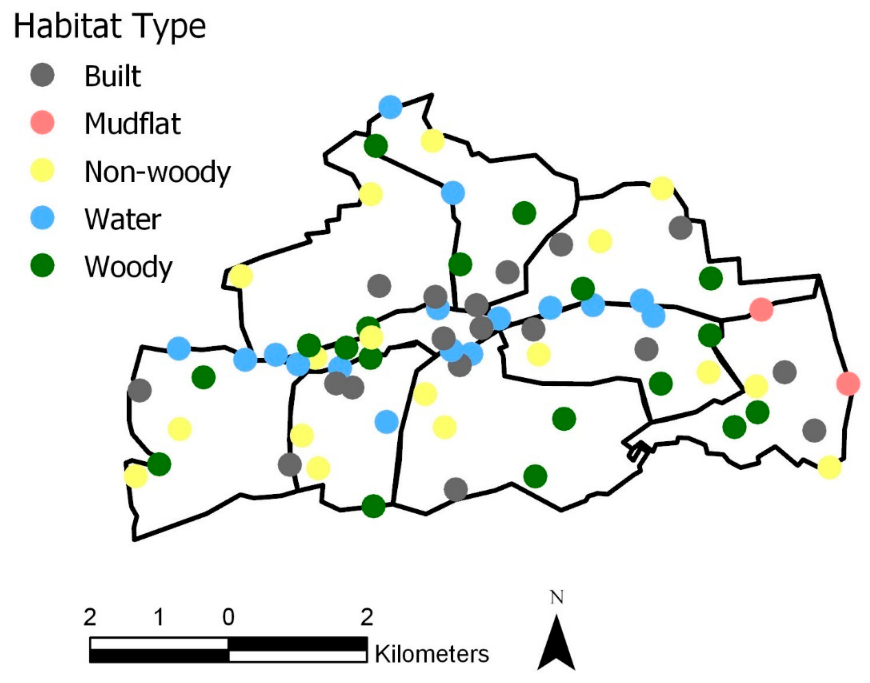
The results of the UGBS land cover classification (Figure 2, Supplementary Information S3) highlight the ability of Sentinel-2 to capture the ‘invisible’ green space of Cork City. The invisible green space in this study is primarily urban gardens, but we also noted several brownfield sites in the north of the city. Our results support previous research that similarly identified the capability for satellite imagery to capture these invisible spaces [34]. This means UGBS classifications can be generated to provide a reliably accurate visualization of the city’s green spaces to support initiatives and policy strategies, such as the previously mentioned Cork City Heritage Plan 2015–2020 and the Draft Cork City Heritage and Biodiversity Plan (2021–2026). The UGBS classification can also aid in identifying corridors in the city, which previous research [2,64] has identified as important to support endangered species in urban regions.
Despite the high accuracy when modelling the green spaces, our results suggest that there is a limitation to using Sentinel-2 imagery for capturing water, which contradicts previous research in urban areas [44]. We posit the reason for such a finding is the scale and configuration of the city. When compared to global cities that have generated classified land cover maps using Sentinel-2, Cork City and the River Lee are relatively small [65,66]. Our classification has been impacted where the river width is less than 10 m, or where overhanging tree canopy, floating and riparian vegetation or shadows prevent the full river width from being viewed within a single pixel. The mixed-pixel challenge in the classification process occurs when the spectral signature averaged over a pixel is more representative of the land cover classes with the higher reflectance values [42], in this case woody and built, compared to the water class which has very low reflectance values at all wavelengths. The spatial resolution also compounds issues in the poor producer accuracy of the water class (Table 3). When multiple surfaces congregate in a tightly-knit urban environment, the 10 m × 10 m pixel sizes of Sentinel-2 data lead to further mixed-pixel contamination, particularly along river edges. However, the combination of a high producer and user accuracy for the other classes provides reassurance that those classes are correctly classified. The other classes, being more generic in their nature, typically extend over multiple pixels in a non-linear form, and thus while there may be some edge effects of mixed pixel misclassification, the internal pixels for each region can be confidently interpreted. Moreover, by using the landscape configuration metrics implemented in FRAGSTATS and including interactions in the regression analysis, it is possible to see what is immediately surrounding the rivers. Blue space was expected to have a mixed impact on bird diversity, and this is displayed in the positive blue-green and negative blue-built interactions found in the regression models (Table 6).
We identified mixed relationships with water and biodiversity, with water forming a negative relationship with richness at 100 m and a positive relationship at 200 m when parameterized using class metrics (Table 5). These results are likely dependent on the blue space type and the habitats that surround it. The edge effect is one such phenomenon that we posit can explain these inverted relationships across scale, as there is a tendency for an increase in species richness and abundance arising from a mixing between two communities [67]. Richness generally increased when blue spaces were flanked by woody riparian corridors, compared to low levels of richness where the river flowed through the city center itself and was surrounded by the built environment (Table 7). Future avenues of research could explore the role of mixed pixels and their inference in the edge effect phenomena, developing a spatially explicit accuracy assessment that accounts for location within the landscape configuration. As such, it is important that individual variables are not considered in isolation in any statistical models, but rather the overall landscape configuration is accounted for. However, our regression models suggest that the presence of water surrounded by built environments should not be entirely discounted.
The interaction between water and CONNECT is a possible indication of how blue space can positively affect bird diversity from a connective standpoint, testing the potential for river systems as connective functions for bird diversities in urban areas [68,69]. In other studies, species richness was found to decline as rivers entered the urban core [68], corroborating our results when land cover was considered as a main effect in the statistical models (Table 5 and Table 6). However, the positive interaction between water and CONNECT corroborates other studies [12,70], where the incorporation of a connectivity metric was found to increase biodiversity. In our study area, the River Lee flows through the city center, where the built environment almost represents an “urban wall” where there is little to no green space, restricting movement of bird diversity (Figure 2). Due to the Lee splitting in two on the north and south side of the city center, it offers two connective networks for birds to freely move between either side of the city and greener pastures, and as such highlights the important of considering the ecology of the city as a whole (supporting [25]), as the unique geography can result in novel ecological patterns that may only be captured at multiple spatial scales [26].
The relationships with green and built spaces were less surprising (Table 5 and Table 6). Green space was shown to have a positive relationship with bird diversity, and by contrast, the built class exhibited negative relationships with bird diversity. These relationships were expected as green space was projected to have a positive impact on bird diversity, particularly woody habitat, while built environment was projected to have a negative impact, as has been found in other studies [2,35,71,72]. For example, our research corroborates the findings of Keten et al. [71] who developed a riparian quality index to quantify the impact on such habitats on avian biodiversity, identifying that as the proportion of urban cover decreases in riparian habitat and is replaced with more natural green coverage, biodiversity increases. However, our results suggest that the built class should not be totally discounted as it can aid bird diversity in the form of providing suitable nesting habitats and alternative food sources [73,74,75]. This is particularly pertinent for Cork City, where a large amount of the green space returned in the UGBS classification was private gardens. The combination of built and ‘invisible’ green space within the wider landscape of Cork is clear in supporting an increased biodiversity. Moreover, the observation of a whitethroat at a brownfield site associated with scrubland habitat further demonstrates the role of invisible green spaces to biodiversity.
One of the main results emanating from these field surveys is that 38% of the species recorded in Cork City are species of conservation concern in Ireland [76]. Of note were swifts, grey wagtails (Motacliia cinerea), meadow pipits (Anthus pratensis) and black-tailed godwits (wintering) on the Red list, while there were 20 species on the Amber list, including barn swallows, sand martins, willow warblers, European starlings (Sturnus vulgaris), and herring gulls (Larus argentatus) (wintering). This information demonstrates how important urban areas such as Cork City can be for species monitoring and management. For example, urban landscapes have become important for many threatened gull species that use buildings for nesting sites [
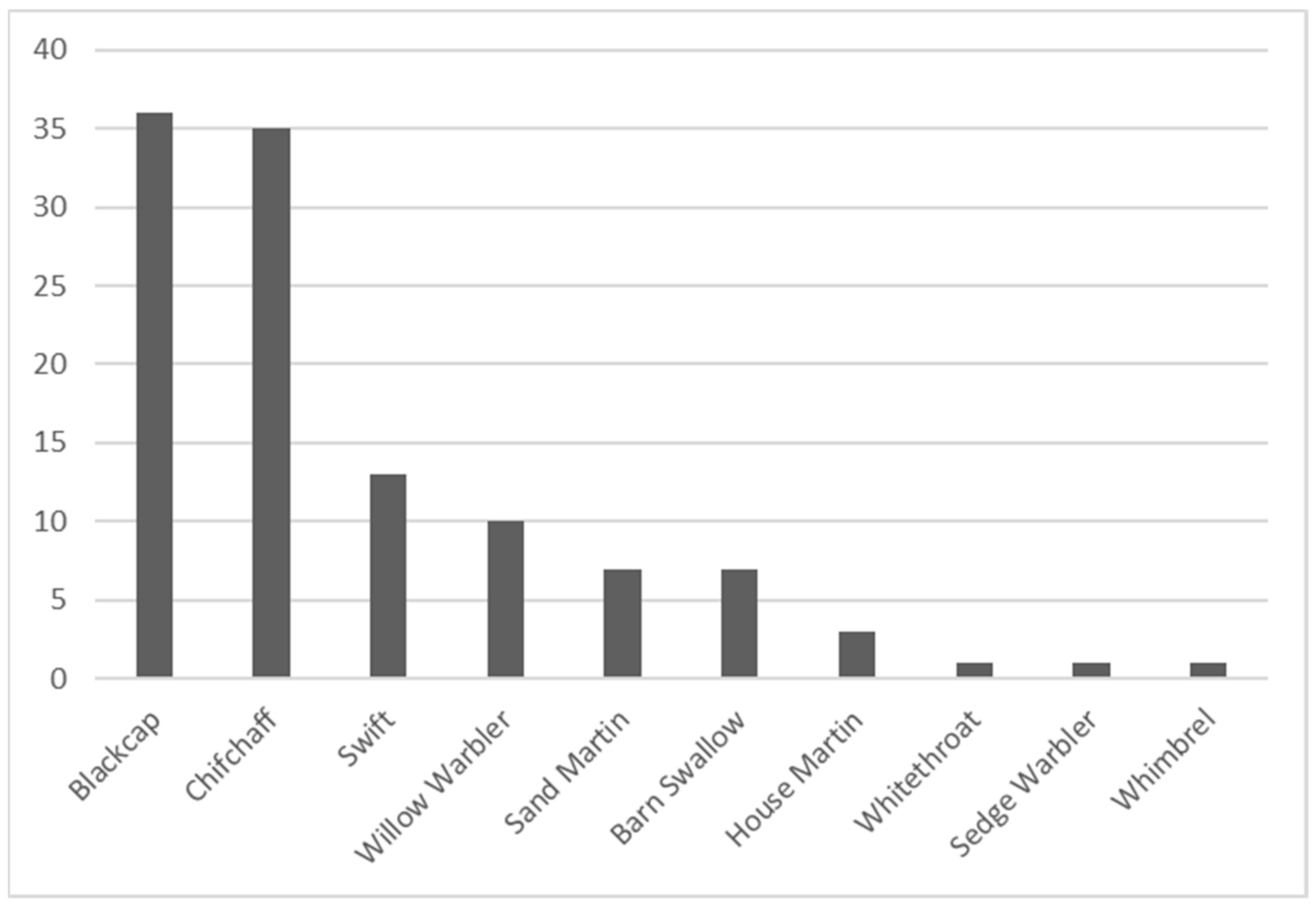
74]; however, building renovations have resulted in a loss of breeding habitat for many other endangered species such as swifts [63]. Urban nest-boxes have been reported as a compensatory measure [77], yet in Cork City the high prevalence of swifts (Figure 4) may be due to the many vacant and derelict buildings [78], although further research at a city scale is needed to quantify how many swifts are supported within the city and specifically where they are nesting. As such, it is important to consider species-specific responses to landscape configurations in urban areas, as important relationships may be overlooked when species are aggregated into an overall biodiversity metric.
It is important to note here that we present our results with some caveats, including the removal of three field surveys in water locations and the potential for more validation points to provide confidence intervals to land cover classifications. Moreover, the issue of detectability in bird surveys is well recognized [55,79,80,81,82], with various considerations required when implementing surveys. Incomplete detectability can be considered less of a concern if a rigorous sampling design is implemented, which reduces the variation in detection probabilities to less than any variation in the population size [83]. We implemented several of the protocols outlined by Hedblom and Soderström [83], such as a consistent calendar period, surveying during peak vocal activity, avoiding adverse weather conditions, only counting birds within our radius, discounting birds that flew high above the site, and waiting a short period upon arrival to the site to begin surveying. The exception to this was that we could not conduct repeat surveys due to time and resource constraints affiliated with this study, although this is not out of line with other studies that have found the efficacy of one count studies to be sufficient [84,85]. However, it should be noted that there will always be uncertainty surrounding detectability even when the number of surveys increases [86].
We decided not to deconstruct our biodiversity metrics into species groups based on detectability or traits as has been suggested for birds and other taxa [79,87]. Instead, to explore any variation and uncertainty associated with slight differences in surveys, we undertook further analysis and grouped the results by zone, taking the average of point counts and landscape variables within a zone, following [7]. For example, the richness values of 16 at site 2 and 10 at site 6 (both woody) were averaged to become 13. We completed this for all classes within each zone, averaging both the response variables and the landscape metrics. We then re-ran our statistical models (Supplementary Information S7). Across both class and landscape metrics, we observed slight differences in the variables returned by the stepAIC process as would be expected when using an information criterion. However, we only reported seven instances where the coefficient inverted, out of all possible combinations of variables (including two-way interactions), which is 36 for the landscape metric model and 10 for the class metric model. Of these seven inversions, only two were significant. The main difference between the original model (Table 6) and the aggregated model (Supplementary Information S7) is that for abundance, water now returns a positive relationship at all scales as opposed to a negative one when considered as a main effect. The aggregation of sites as opposed to repeat counts may be one such artefact for returning different relationships, as we are combining results from different water environments as opposed to repeating counts at the exact same location. However, such findings do not contradict the main conclusions drawn from our results, as our original interpretation that land cover classes should not be considered in isolation from the surrounding landscape configuration remain due to positive water and connectivity interactions. As the results of this aggregation largely concur with our original models, and due to the fact that such an aggregation reduces our n substantially (n = 35), as well as the uncertainty from treating different locations as repeat surveys, we prefer to report the results of our original model, with the caveat that such abundance metrics should be treated with caution due to lack of repeat surveys.
Another perspective that warrants future research is to classify different tree cover types such as coniferous and deciduous trees, or applying a land use classification to different green spaces such as parks, cemeteries, and gardens. The coniferous and deciduous types of wooded areas would make a difference when it comes to bird diversity [79]. This is because certain species or habitat specialists prefer coniferous woodland, such as coal tits (Periparus ater), crossbills (Loxia curvirosta) and goldcrests (Regulus regulus) compared to deciduous woodland which would have a larger assortment of species [88]. A classification of the various green space types in Cork City coupled with survey results for each green space type would also provide key information on bird diversity that could help the necessary stakeholders develop and distribute information on biodiversity and heritage for the Draft Cork City Heritage and Biodiversity Plan 2021–2026. It was not possible to discriminate between coniferous and deciduous woodland, however, as the spatial resolution was not adequate or fine enough to allow for such identifications. The lack of cloud free imagery for the winter months also played a part in this as it may have been possible to notice the lack of leaves on deciduous, compared to coniferous trees. Satellite imagery with finer resolution could possibly be more effective in classifying the vegetation types such as deciduous and coniferous vegetation and produce a more accurate result for water [41,89,90].

5. Conclusions

With over 1 million species at risk of extinction globally [9], there is a pressing need to identify the optimal spatial configuration of landscapes to support biodiversity. Here, a combination of remote sensing, field surveys, and landscape metrics was used to explore the role of landscape configuration, specifically urban green and blue space, on bird biodiversity patterns in Cork City. Remote sensing was identified as an effective tool to identify areas of ‘invisible’ green space, such as gardens, with green space (both woody and non-woody) accounting for almost two-thirds of the landscape (Figure 2). FRAGSTATS was then used to capture landscape metrics regarding the spatial configuration of the study area, at a city scale and at three spatial extents for each field site. It was found that as the scale increased, connectivity often decreased as landscapes became dominated by built cover (Figure 5). Field surveys recorded 62 species in the city (Figure 3 and Figure 4), with 38% listed as species of conservation concern in Ireland, highlighting how urban spaces can provide habitats for vulnerable species, particularly when there is a plethora of connected and interspersed green and blue spaces. GLMs revealed that green space was a significant driver in increasing species richness and abundance, while blue space produced inversions in coefficient estimates (Table 5 and Table 6). Green space was found to be one of the main drivers in increasing species richness and abundance, particularly the woody class. A mixed relationship was encountered between blue space and bird diversity, with the edge effect phenomenon posited as playing a key role in determining such relationships. Where blue space had a significantly positive impact on bird diversity, woodland was an adjacent habitat, whereas significantly negative impacts when the built class was the adjacent habitat (Table 5 and Table 6). Generally, the built class was found to be detrimental to bird diversity, but we provide exceptions to this rule, particularly due to the availability of nest substrates and provision of smaller ‘invisible’ green spaces, such as urban gardens and brownfield sites, in supporting species of conservation concern. The positive interaction between water and the CONNECT metric indicates the potential of blue corridors as a connective function in the city. However, this is dependent on the relative scales of the blue corridors themselves, as the wider a river is the less likely a bird will travel over it. The River Lee in Cork City splits either side of the city center creating two smaller channels which act as connective corridors for bird diversity, particularly the north channel which is flanked by vegetative riparian corridors which positively influences bird diversity (Table 6). The role of interspersed blue and green space, and the need to consider these as separate entities is clear for future urban planning.

Supplementary Materials

The following are available online at https://0-www-mdpi-com.brum.beds.ac.uk/article/10.3390/geographies1030013/s1. Supplementary Information S1: Zonal delineation and sampling locations. Supplementary Information S2: Information on landscape metrics with full equations. Supplementary Information S3: Land cover classification product for Cork City, Ireland. Supplementary Information S4: Field Survey Data. Supplementary Information S5: T-test results for scale comparison of landscape metrics. Supplementary Information S6: Ancillary statistics. Supplementary Information S7: Results of GLM fit with zonal aggregated data.

Author Contributions

Conceptualization, L.L., F.C., and P.H.; Methodology, L.L., F.C., and P.H.; formal analysis, L.L.; data curation, L.L.; writing—original draft preparation, L.L., F.C., and P.H. All authors have read and agreed to the published version of the manuscript.

Funding

This research received no external funding.

Institutional Review Board Statement

Ethical review and approval waived for this study, as all data collection was observation only.

Informed Consent Statement

Not applicable.

Data Availability Statement

All data have been made available in the Supplementary Information.

Acknowledgments

We would like to thank the editors and reviewers for their comments and suggestions.

Conflicts of Interest

The authors declare no conflict of interest.

References

  1. Pataki, D.E. Grand challenges in urban ecology. Front. Ecol. Evol. 2015, 3, 57. [Google Scholar] [CrossRef] [Green Version]
  2. Mörtberg, U.; Wallentinus, H.G. Red-listed forest bird species in an urban environment—Assessment of green space corridors. Landsc. Urban Plan. 2000, 50, 215–226. [Google Scholar] [CrossRef]
  3. Rudd, H.; Vala, J.; Schaefer, V. Importance of backyard habitat in a comprehensive biodiversity conservation strategy: A connectivity analysis of urban green spaces. Restor. Ecol. 2002, 10, 368–375. [Google Scholar] [CrossRef] [Green Version]
  4. Dearborn, D.C.; Kark, S. Motivations for conserving urban biodiversity. Conserv. Biol. 2010, 24, 432–440. [Google Scholar] [CrossRef] [PubMed]
  5. Kong, F.; Yin, H.; Nakagoshi, N.; Zong, Y. Urban green space network development for biodiversity conservation: Identification based on graph theory and gravity modeling. Landsc. Urban Plan. 2010, 95, 16–27. [Google Scholar] [CrossRef]
  6. Lepczyk, C.A.; Aronson, M.F.; Evans, K.L.; Goddard, M.A.; Lerman, S.B.; MacIvor, J.S. Biodiversity in the city: Fundamental questions for understanding the ecology of urban green spaces for biodiversity conservation. BioScience 2017, 67, 799–807. [Google Scholar] [CrossRef] [Green Version]
  7. Holloway, P.; Field, R. Can rock-rubble groynes support similar intertidal ecological communities to natural rocky shores? Land 2020, 9, 131. [Google Scholar] [CrossRef]
  8. Russo, A.; Cirella, G.T. Urban Ecosystem Services: New Findings for Landscape Architects, Urban Planners, and Policymakers. Land 2021 2021, 10, 88. [Google Scholar]
  9. Díaz, S.; Settele, J.; Brondízio, E.S.; Ngo, H.T.; Guèze, M.; Agard, J.; Arneth, A.; Balvanera, P.; Brauman, K.A.; Butchart, S.H.M.; et al. (Eds.) IPBES 2019: Summary for Policymakers of the Global Assessment Report on Biodiversity and Ecosystem Services of the Intergovernmental Science-Policy Platform on Biodiversity and Ecosystem Services; IPBES Secretariat: Bonn, Germany, 2019; 56. [Google Scholar] [CrossRef]
  10. Turner, M.G.; Gardner, R.H. Landscape Ecology in Theory and Practice; Springer: New York, NY, USA, 2001; Volume 401. [Google Scholar]
  11. Bury, J.; Mark, B.G.; Carey, M.; Young, K.R.; McKenzie, J.M.; Baraer, M.; French, A.; Polk, M.H. New geographies of water and climate change in Peru: Coupled natural and social transformations in the Santa River watershed. Ann. Assoc. Am. Geogr. 2013, 103, 363–374. [Google Scholar] [CrossRef] [Green Version]
  12. Li, H.; Chen, W.; He, W. Planning of green space ecological network in urban areas: An example of Nanchang, China. Int. J. Environ. Res. Public Health 2015, 12, 12889–12904. [Google Scholar] [CrossRef] [PubMed] [Green Version]
  13. Lamine, S.; Petropoulos, G.P.; Singh, S.K.; Szabó, S.; Bachari, N.E.I.; Srivastava, P.K.; Suman, S. Quantifying land use/land cover spatio-temporal landscape pattern dynamics from Hyperion using SVMs classifier and FRAGSTATS®. Geocarto Int. 2018, 33, 862–878. [Google Scholar] [CrossRef]
  14. Cushman, S.; McGarigal, K. Patterns in the species–environment relationship depend on both scale and choice of response variables. Oikos 2004, 105, 117–124. [Google Scholar] [CrossRef]
  15. Geary, M.; Fielding, A.H.; Marsden, S.J. Designing mosaic landscapes for B lack G rouse T etrao tetrix using multi-scaled models. Ibis 2013, 155, 792–803. [Google Scholar] [CrossRef]
  16. Holloway, P. Aggregating the conceptualization of movement data better captures real world and simulated animal–environment relationships. Int. J. Geogr. Inf. Sci. 2020, 34, 1585–1606. [Google Scholar] [CrossRef]
  17. Liu, M.; Li, X.; Song, D.; Zhai, H. Evaluation and Monitoring of Urban Public Greenspace Planning Using Landscape Metrics in Kunming. Sustainability 2021, 13, 3704. [Google Scholar] [CrossRef]
  18. Oliveira Hagen, E.; Hagen, O.; Ibáñez-Álamo, J.D.; Petchey, O.L.; Evans, K.L. Impacts of Urban Areas and Their Characteristics on Avian Functional Diversity. Front. Ecol. Evol. 2017, 5, 84. [Google Scholar] [CrossRef] [Green Version]
  19. Isaksson, C. Impact of Urbanization on Birds. In Bird Species; Tietze, D., Ed.; Fascinating Life Sciences; Springer: Cham, Switzerland, 2018. [Google Scholar] [CrossRef] [Green Version]
  20. Pei, N.; Wang, C.; Jin, J.; Jia, B.; Chen, B.; Qie, G.; Qiu, E.; Gu, L.; Sun, R.; Li, J.; et al. Long-term afforestation efforts increase bird species diversity in Beijing, China. Urban For. Urban Green. 2018, 29, 88–95. [Google Scholar] [CrossRef]
  21. Shoffner, A.; Wilson, A.M.; Tang, W.; Gagné, S.A. The relative effects of forest amount, forest configuration, and urban matrix quality on forest breeding birds. Sci. Rep. 2018, 8, 1–12. [Google Scholar]
  22. Lomolino, M.V. The species-area relationship: New challenges for an old pattern. Prog. Phys. Geogr. 2001, 25, 1–21. [Google Scholar]
  23. Fahrig, L. Ecological responses to habitat fragmentation per se. Annu. Rev. Ecol. Evol. Syst. 2017, 48, 1–23. [Google Scholar] [CrossRef]
  24. Villard, M.A.; Trzcinski, M.K.; Merriam, G. Fragmentation effects on forest birds: Relative influence of woodland cover and configuration on landscape occupancy. Conserv. Biol. 1999, 13, 774–783. [Google Scholar] [CrossRef] [Green Version]
  25. Soifer, L.G.; Donovan, S.K.; Brentjens, E.T.; Bratt, A.R. Piecing together cities to support bird diversity: Development and forest edge density affect bird richness in urban environments. Landsc. Urban Plan. 2021, 213, 104122. [Google Scholar] [CrossRef]
  26. Kupfer, J.A. Landscape ecology and biogeography: Rethinking landscape metrics in a post-FRAGSTATS landscape. Prog. Phys. Geogr. 2012, 36, 400–420. [Google Scholar] [CrossRef]
  27. Turner, M.G.; O’Neill, R.V.; Gardner, R.H.; Milne, B.T. Effects of changing spatial scale on the analysis of landscape pattern. Landsc. Ecol. 1989, 3, 153–162. [Google Scholar] [CrossRef]
  28. Rahbek, C.; Graves, G.R. Multiscale assessment of patterns of avian species richness. Proc. Natl. Acad. Sci. USA 2001, 98, 4534–4539. [Google Scholar] [CrossRef] [Green Version]
  29. Willis, K.J.; Whittaker, R.J. Species diversity—Scale matters. Science 2002, 295, 1245–1248. [Google Scholar] [CrossRef] [PubMed]
  30. Kumar, S.; Simonson, S.E.; Stohlgren, T.J. Effects of spatial heterogeneity on butterfly species richness in Rocky Mountain National Park, CO, USA. Biodivers. Conserv. 2009, 18, 739–763. [Google Scholar] [CrossRef]
  31. Holloway, P.; Miller, J. Exploring spatial scale, autocorrelation and nonstationarity of bird species richness patterns. ISPRS Int. J. GeoInf. 2015, 4, 783–798. [Google Scholar] [CrossRef] [Green Version]
  32. Croci, S.; Butet, A.; Georges, A.; Aguejdad, R.; Clergeau, P. Small urban woodlands as biodiversity conservation hot-spot: A multi-taxon approach. Landsc. Ecol. 2008, 23, 1171–1186. [Google Scholar] [CrossRef]
  33. Van Heezik, Y.; Freeman, C.; Porter, S.; Dickinson, K.J. Garden size, householder knowledge, and socio-economic status influence plant and bird diversity at the scale of individual gardens. Ecosystems 2013, 16, 1442–1454. [Google Scholar] [CrossRef]
  34. Feltynowski, M.; Kronenberg, J.; Bergier, T.; Kabisch, N.; Łaszkiewicz, E.; Strohbach, M.W. Challenges of urban green space management in the face of using inadequate data. Urban For. Urban Green. 2018, 31, 56–66. [Google Scholar] [CrossRef]
  35. Dragos, M.; Petrescu, A.; Merciu, G.L. Analysis of vegetation from satellite images correlated to the bird species presence of the state of health of the ecosystems of Bucharest during the period from 1991 to 2006. Geogr. Pannonica 2017, 21, 925. [Google Scholar] [CrossRef] [Green Version]
  36. Rafiee, R.; Mahiny, A.S.; Khorasani, N. Assessment of changes in urban green spaces of Mashad city using satellite data. Int. J. Appl. Earth Obs. Geoinf. 2009, 11, 431–438. [Google Scholar] [CrossRef]
  37. Kabisch, N.; Selsam, P.; Kirsten, T.; Lausch, A.; Bumberger, J. A multisensor and multi-temporal remote sensing approach to detect land cover change dynamics in heterogeneous urban landscapes. Ecol. Indic. 2019, 99, 273–282. [Google Scholar] [CrossRef]
  38. Van, T.T.; Tran, N.D.H.; Bao, H.D.X.; Phuong, D.T.T.; Hoa, P.K.; Han, T.T.N. Optical remote sensing method for detecting urban green space as indicator serving city sustainable development. Proceedings 2017, 2, 140. [Google Scholar] [CrossRef] [Green Version]
  39. Zhou, W.; Wang, J.; Qian, Y.; Pickett, S.T.; Li, W.; Han, L. The rapid but “invisible” changes in urban greenspace: A comparative study of nine Chinese cities. Sci. Total Environ. 2018, 627, 1572–1584. [Google Scholar] [CrossRef] [PubMed]
  40. Haas, J.; Ban, Y. Urban land cover and ecosystem service changes based on Sentinel-2A MSI and Landsat TM Data. IEEE J. Sel. Top. Appl. Earth Obs. Remote Sens. 2018, 11, 485–497. [Google Scholar] [CrossRef]
  41. Wang, J.; Zhou, W.; Qian, Y.; Li, W.; Han, L. Quantifying and characterizing the dynamics of urban greenspace at the patch level: A new approach using objectbased image analysis. Remote Sens. Environ. 2018, 204, 94–108. [Google Scholar] [CrossRef]
  42. Rosina, K.; Kopecká, M. Mapping of urban green spaces using Sentinel-2A data: Methodical aspects. In Proceedings of the 6th International Conference on Cartography and GIS, Albena, Bulgaria, 13–17 June 2016; Bulgarian Cartographic Association: Sofia, Bulgaria, 2016; pp. 562–568. [Google Scholar]
  43. Kopecká, M.; Szatmári, D.; Rosina, K. Analysis of urban green spaces based on Sentinel-2A: Case studies from Slovakia. Land 2017, 6, 25. [Google Scholar] [CrossRef] [Green Version]
  44. Vatseva, R.; Kopecka, M.; Otahel, J.; Rosina, K.; Kitev, A.; Genchev, S. Mapping urban green spaces based on remote sensing data: Case studies in Bulgaria and Slovakia. In Proceedings of the 6th International Conference on Cartography and GIS, Albena, Bulgaria, 13–17 June 2016; pp. 569–578. [Google Scholar]
  45. Central Statistics Office 2017. Census 2016 Summary Results—Part 1. Available online: https://www.cso.ie/en/media/csoie/newsevents/documents/census2016summaryresultspart1/Census2016SummaryPart1.pdf (accessed on 26 October 2021).
  46. McCarthy, G.D.; Gleeson, E.; Walsh, S. The influence of ocean variations on the climate of Ireland. Weather 2015, 70, 242–245. [Google Scholar] [CrossRef] [Green Version]
  47. Cork City Council. Nature in the City: A Guide to Biodiversity in Cork. 2009. Available online: https://www.corkcity.ie/en/media-folder/heritage/nature-in-the-city-1.pdf (accessed on 26 October 2021).
  48. Cork City Council. Cork City Development Plan 2015–2021. 2019. Available online: http://www.corkcitydevelopmentplan.ie/ (accessed on 26 October 2021).
  49. Earth Explorer; 2000; FS; 083-00; Geological Survey (U.S.). Available online: https://earthexplorer.usgs.gov/ (accessed on 26 October 2021).
  50. Ordnance Survey Ireland, 2019, GeoHive. Available online: https://www.geohive.ie/ (accessed on 26 October 2021).
  51. Olofsson, P.; Foody, G.M.; Herold, M.; Stehman, S.V.; Woodcock, C.E.; Wulder, M.A. Good practices for estimating area and assessing accuracy of land change. Remote Sens. Environ. 2014, 148, 42–57. [Google Scholar] [CrossRef]
  52. Volpato, G.H.; Lopes, E.V.; Mendonça, L.B.; Boçon, R.; Bisheimer, M.V.; Serafini, P.P.; Anjos, L.D. The use of the point count method for bird survey in the Atlantic Forest. Zoologia (Curitiba) 2009, 26, 74–78. [Google Scholar] [CrossRef]
  53. Nalwanga, D.; Pomeroy, D.; Vickery, J.; Atkinson, P.W. A comparison of two survey methods for assessing bird species richness and abundance in tropical farmlands. Bird Study 2012, 59, 83–95. [Google Scholar] [CrossRef]
  54. Saskatchewan Breeding Bird Atlas. Instructions for Point Counts. 2017. Available online: https://sk.birdatlas.ca/wp-content/uploads/2020/05/SK-Breeding-Bird-Atlas-Instructions-for-Point-Counts-2020-05-08.pdf (accessed on 26 October 2021).
  55. Van Heezik, Y.; Seddon, P.J. Accounting for detectability when estimating avian abundance in an urban area. N. Z. J. Ecol. 2012, 36, 1. [Google Scholar]
  56. Bibby, C.J.; Burgess, N.D.; Hillis, D.M.; Hill, D.A.; Mustoe, S. Bird Census Techniques; Academic Press: London, UK, 2000. [Google Scholar]
  57. Environmental Protection Agency. WFD River Water Bodies—Cycle 2—27/04/2017. 2017. Available online: https://gis.epa.ie/GetData/Download (accessed on 1 May 2019).
  58. McGarigal, K.; Cushman, S.A.; Ene, E. FRAGSTATS v4: Spatial Pattern Analysis Program for Categorical and Continuous Maps; Computer Software Program Produced by the Authors at the University of Massachusetts; University of Massachusetts: Amherst, MA, USA, 2012; Available online: http://www.umass.edu/landeco/research/fragstats/fragstats.html (accessed on 26 October 2021).
  59. R Core Team. R: A Language and Environment for Statistical Computing; Foundation for Statistical Computing: Vienna, Austria, 2019; Available online: https://www.R-project.org/ (accessed on 26 October 2021).
  60. Fox, J.; Weisberg, S. An R Companion to Applied Regression, 3rd ed.; Sage: Thousand Oaks, CA, USA, 2019. [Google Scholar]
  61. Venables, W.N.; Ripley, B.D. Modern Applied Statistics with S-Plus, 4th ed.; Springer: New York, NY, USA, 2002. [Google Scholar]
  62. Lewis, L.J.; Coombes, D.; Burke, B.; O’Halloran, J.; Walsh, A.; Tierney, T.D.; Cummins, S. Countryside Bird Survey: Status and Trends of Common and Widespread Breeding Birds 1998–2016; Irish Wildlife Manuals, No. 115; National Parks and Wildlife Service, Department of Culture, Heritage and the Gaeltacht: Dublin, Ireland, 2019. [Google Scholar]
  63. Birdwatch Ireland. Irelands Birds. 2019. Available online: https://birdwatchireland.ie/irelands-birds-birdwatch-ireland/list-of-irelands-birds/ (accessed on 26 October 2021).
  64. Wang, H.; Pei, Z. Urban Green Corridors Analysis for a Rapid Urbanization City Exemplified in Gaoyou City, Jiangsu. Forests 2020, 11, 1374. [Google Scholar] [CrossRef]
  65. Zhang, T.; Su, J.; Xu, Z.; Luo, Y.; Li, J. Sentinel-2 Satellite Imagery for Urban Land Cover Classification by Optimized Random Forest Classifier. Appl. Sci. 2021, 11, 543. [Google Scholar] [CrossRef]
  66. Qiu, C.; Mou, L.; Schmitt, M.; Zhu, X.X. Fusing Multiseasonal Sentinel-2 Imagery for Urban Land Cover Classification with Multibranch Residual Convolutional Neural Networks. IEEE Geosci. Remote Sens. Lett. 2020, 17, 1787–1791. [Google Scholar] [CrossRef]
  67. Odum, E.P. Fundamentals of Ecology, 2nd ed.; Saunders: Philadelphia, PA, USA, 1958. [Google Scholar]
  68. Dallimer, M.; Rouquette, J.R.; Skinner, A.M.; Armsworth, P.R.; Maltby, L.M.; Warren, P.H.; Gaston, K.J. Contrasting patterns in species richness of birds, butterflies and plants along riparian corridors in an urban landscape. Divers. Distrib. 2012, 18, 742–753. [Google Scholar] [CrossRef]
  69. Tremblay, M.A.; St. Clair, C.C. Factors affecting the permeability of transportation and riparian corridors to the movements of songbirds in an urban landscape. J. Appl. Ecol. 2009, 46, 1314–1322. [Google Scholar] [CrossRef]
  70. Bierwagen, B.G. Connectivity in urbanizing landscapes: The importance of habitat configuration, urban area size, and dispersal. Urban Ecosyst. 2007, 10, 2942. [Google Scholar] [CrossRef]
  71. Keten, A.; Eroglu, E.; Kaya, S.; Anderson, J.T. Bird diversity along a riparian corridor in a moderate urban landscape. Ecol. Indic. 2020, 118, 106751. [Google Scholar] [CrossRef]
  72. Sandström, U.G.; Angelstam, P.; Mikusiński, G. Ecological diversity of birds in relation to the structure of urban green space. Landsc. Urban Plan. 2006, 77, 39–53. [Google Scholar] [CrossRef]
  73. Wilson, J.; Carmody, M. Freshwater Birds of Ireland; Collins Press: Cork, Ireland, 2011. [Google Scholar]
  74. Spelt, A.; Williamson, C.; Shamoun-Baranes, J.; Shepard, E.; Rock, P.; Windsor, S. Habitat use of urban-nesting lesser black-backed gulls during the breeding season. Sci. Rep. 2019, 9, 10527. [Google Scholar] [CrossRef] [PubMed]
  75. Caballero, I.C.; Bates, J.M.; Hennen, M.; Ashley, M.V. Sex in the City: Breeding Behavior of Urban Peregrine Falcons in the Midwestern US. PLoS ONE 2016, 11, e0159054. [Google Scholar] [CrossRef] [PubMed]
  76. Gilbert, G.; Stanbury, A.; Lewis, L. Birds of Conservation Concern in Ireland 2020–2026. Ir. Birds 2021, 9, 523–544. [Google Scholar]
  77. Schaub, T.; Meffert, P.J.; Kerth, G. Nest-boxes for Common Swifts Apus apus as compensatory measures in the context of building renovation: Efficacy and predictors of occupancy. Bird Conserv. Int. 2016, 26, 164. [Google Scholar] [CrossRef] [Green Version]
  78. Holloway, P.; Kenna, T.; Linehan, D.; O’Connor, R.; Bradley, H.; O’Mahony, B.; Pinkham, R. Active learning using a smartphone app: Analysing land use patterns in Cork City, Ireland. J. Geogr. High. Educ. 2020, 45, 47–62. [Google Scholar] [CrossRef]
  79. Sweeney, O.F.M.; Wilson, M.W.; Irwin, S.; Kelly, T.C.; O’Halloran, J. Are bird density, species richness and community structure similar between native woodlands and non-native plantations in an area with a generalist bird fauna? Biodivers. Conserv. 2010, 19, 2329–2342. [Google Scholar] [CrossRef]
  80. Dorazio, R.M.; Royle, J.A.; Söderström, B.; Glimskär, A. Estimating species richness and accumulation by modeling species occurrence and detectability. Ecology 2006, 87, 842–854. [Google Scholar] [CrossRef] [Green Version]
  81. Gu, W.; Swihart, R.K. Absent or undetected? Effects of non-detection of species occurrence on wildlife–habitat models. Biol. Conserv. 2004, 116, 195–203. [Google Scholar] [CrossRef]
  82. McGrath, T.; Guillera-Arroita, G.; Lahoz-Monfort, J.J.; Osborne, W.; Hunter, D.; Sarre, S.D. Accounting for detectability when surveying for rare or declining reptiles: Turning rocks to find the grassland earless dragon in Australia. Biol. Conserv. 2015, 182, 53–62. [Google Scholar] [CrossRef]
  83. Hedblom, M.; Söderström, B. Landscape effects on birds in urban woodlands: An analysis of 34 Swedish cities. J. Biogeogr. 2010, 37, 1302–1316. [Google Scholar] [CrossRef]
  84. Haila, Y.; Kuusela, S. Eficiency of one-visit censuses of bird communities breeding on small islands. Ornis Scandanvia 1982, 13, 17–24. [Google Scholar] [CrossRef]
  85. Ralph, C.J.; Sauer, J.R.; Droege, S. Monitoring Bird Populations by Point Counts; General Technical Report PSW-GTR-149; US Department of Agriculture, Forest Service, Pacific Southwest Research Station: Albany, CA, USA, 1995; 187p. [Google Scholar]
  86. Pomeroy, D.; Platz, E.; Platz, K.; Lack, P.; Gottschalk, T.K. The problems of recording bird numbers in the breeding season as pairs. Ornithol. Sci. 2018, 17, 69–78. [Google Scholar] [CrossRef]
  87. Meyer, T.; Holloway, P.; Christiansen, T.B.; Miller, J.A.; D’Odorico, P.; Okin, G.S. An assessment of multiple drivers determining woody species composition and structure: A case study from the Kalahari, Botswana. Land 2019, 8, 122. [Google Scholar] [CrossRef] [Green Version]
  88. Nairn, R.; O’Halloran, J. Bird Habitats in Ireland; Collins Press: Cork, Ireland, 2012. [Google Scholar]
  89. Qian, Y.; Zhou, W.; Yu, W.; Pickett, S.T. Quantifying spatiotemporal pattern of urban greenspace: New insights from high resolution data. Landsc. Ecol. 2015, 30, 1165–1173. [Google Scholar] [CrossRef]
  90. Giezen, M.; Balikci, S.; Arundel, R. Using Remote Sensing to Analyse Net Land-Use Change from Conflicting Sustainability Policies: The Case of Amsterdam. ISPRS Int. J. Geo-Inf. 2018, 7, 381. [Google Scholar] [CrossRef] [Green Version]
Figure 1. The location of the 72 sites within the 9 zones that were surveyed for this research with the Cork City boundary.
Geographies 01 00013 g001
Figure 2. Classified map of urban green, blue, grey, and brown space in Cork City, with red ellipses highlighting some of the regions where single pixels of wood cover were classified in pixels where surface water of the river could not be detected.
Geographies 01 00013 g002
Figure 3. Average bird species richness and abundance recorded from each habitat class.
Geographies 01 00013 g003
Figure 4. The frequency of summer migrants recorded during the field surveys.
Geographies 01 00013 g004
Figure 5. Change in mean landscape metrics derived from FRAGSTATS at each scale (50 m, 100 m and 200 m) with 95% confidence intervals for (a) total area (TA), (b) proportion of like adjacencies (PLADJ), (c) contagion (CONTAG), (d) cohesion (COHESION), (e) connectivity (CONNECT), (f) Simpson’s diversity index (SIDI), and (g) Shannon’s diversity index (SHDI).
Geographies 01 00013 g005
Table 1. Landscape metrics code, description, ecological justification, and value, adapted from McGarigal et al. [58]. Full equations available in Supplementary Information S2.
MetricDescriptionEcological JustificationValue
Total Area (CA)The sum of the areas (m2) of all patches for the corresponding patch type.An increase in area is related to an increase in diversity Greater than 0—no limit
Percentage of landscape (PLAND)The percentage of the landscape comprised of the corresponding patch type.Measures landscape composition which can be an important characteristic in identifying fragmentation or habitat loss.Between 0 and 100—Approaches 0 when corresponding patch type becomes increasingly rare and 100 when entire landscape consists of a single patch type
Total Area (TA)The sum of the areas (m2) of the landscape.An increase in area is related to an increase in diversityGreater than 0—no limit
Connectance Index (CONNECT)The number of functional joins between all patches of the corresponding patch type.A measure of connectivity that defines the number of functional joins between patches of the corresponding patch type, where each pair of patches is either connected or not.Between 0 and 100—0 represents a single patch, 100 when every patch is connected
Contagion (CONTAG)Minus the sum of the proportional abundance of each patch type, which is then multiplied by the proportion of adjacencies between cells of that patch type.A measure of dispersion and interspersion of patch types, which provides information on habitat variability and is inversely related to edge densities in a landscapeBetween 0 and 100—0 when corresponding patch type is maximally disaggregated, 100 when corresponding patch type is maximally aggregated
Proportion of Like Adjacencies (PLADJ)The number of like adjacencies involving the focal class, which is then divided by the total cell adjacencies involving the focal class. Reported as a percentage.A measure of connectivity that quantifies the amount of adjacent patches that are similar within the landscapeBetween 0 and 100—0 when corresponding patch type is maximally disaggregated, 100 when the landscape consists of a single patch
Patch Cohesion Index (COHESION)This is one minus the sum of patch perimeter, divided by the sum of patch perimeter times the square root of patch area for patches of the corresponding patch type, which is then divided by 1 minus 1 over the square root of the total number of cells in the landscape. Reported as a percentage.A measure of connectivity that quantifies the physical connectedness of the corresponding patch typeBetween 0 and 100, with increasing values representing more aggregated/cohesion through the landscape
Shannon’s Diversity Index (SHDI)Proportional abundance of each patch type multiplied by that proportion.diversity metrics, and both measure the high or low landcover diversity present in the landscapeBetween 0 and 1—0 when the landscape contains only 1 patch, 1 when the distribution of area among patch types is perfectly even
Simpson’s Diversity Index (SIDI)One minus the sum, across all patch types, of the proportional abundance of each patch type, squared.diversity metrics, and both measure the high or low landcover diversity present in the landscapeBetween 0 and 1—0 when the landscape contains only 1 patch, SIDI approaches 1 as the number of different patch types increases
Table 2. The ground reference table, displaying the total landscape composition of Cork City.
ClassTotal in Cork City (%)
Unclassified0.93
Built32.71
Mudflat9.35
Non-Woody28.97
Water5.61
Woody22.43
Table 3. The error matrix, producer and user accuracy results for each class from the accuracy assessment of the classified image. GCP refers to Ground Control Points.
BuiltMudflatNon-WoodyWaterWoodyUser Accuracy (%)
Unclassified00100
Built40008083.33
Mudflat010000100.00
Non-woody00395088.64
Water000100100.00
Woody00073081.08
Producer Accuracy (%)100.00100.0097.5033.33100.00
Total GCP4010403030
Table 4. Landscape metrics reported for Cork City at a city-level scale.
MetricValueInterpretation
TA3974.34The overall size of the city.
CONTAG46.48A mix of aggregated and dispersed patch types.
PLADJ67.75Proposes there is more aggregation of patches in the city than dispersion.
CONNECT0A lack of connectivity between patch types within the city.
COHESION98.90High cohesion between patch types in the city.
SHDI0.97A high diversity of land covers within the city.
SIDI0.57A more neutral diversity in the land covers within the city.
Table 5. Coefficient and standard errors for richness and abundance when parameterized using the class metrics. * p < 0.01, ** p < 0.001. No corrections for multiple tests were included. Model reported is a result of forwards and backwards AIC selection.
50 m100 m200 m
RichnessAbundanceRichnessAbundanceRichnessAbundance
VariableEstimateStd. ErrorEstimateStd. ErrorEstimateStd. ErrorEstimateStd. ErrorEstimateStd. ErrorEstimateStd. Error
Intercept14.17 **0.6027.94 **1.576.33 **0.79713.74 **2.0215.76 **0.92−14.6121.22
Woody 0.08 *0.030.120.08 0.52 *0.20
Water −0.190.09−0.580.250.080.082.41 *0.19
Non-Woody 0.09 **0.020.16 **0.04 0.520.23
Built−0.08 **0.01−0.15 **0.03 −0.10 **0.18
Woody:Water 0.02 *0.0060.05 **0.02
Water:Non-Woody −0.04 *0.02
Water:Built −0.010.00−0.03 *0.01
Non-Woody:Built −0.000.00
Table 6. Coefficient and standard errors for richness and abundance when parameterized using the landscape metrics. * p < 0.01, ** p < 0.001. No corrections for multiple tests were included. Model reported is a result of forwards and backwards AIC selection.
50 m100 m200 m
RichnessAbundanceRichnessAbundanceRichnessAbundance
VariableEstimateStd. ErrorEstimateStd. ErrorEstimateStd. ErrorEstimateStd. ErrorEstimateStd. ErrorEstimateStd. Error
Intercept15.516.7241.36 **9.954.20 **1.2153.8523.32132.34 *46.21340.50 *112.60
Water −0.040.880.010.23−0.380.29−0.36 *0.12−0.310.29
Woody −1.420.600.220.120.110.09 0.33 **0.09
Non-Woody 0.06 *0.020.16 **0.04 0.27 **0.06
Built−0.08 **0.01−0.12 **0.05 −0.10 **0.02
CONTAG −2.11 **0.57−4.04 *1.41
CONNECT −0.020.050.030.03 11.40 *4.270.000.32
PLADJ−0.030.08−0.190.13 −0.420.25−1.430.61−4.29 *1.48
SHDI−10.886.85 5.022.32−11.787.51−83.63 *31.29−164.0076.18
Woody:PLADJ 0.020.01
Water:Built −0.02 *0.01
Water:CONNECT 0.020.010.04 **0.01 0.06 *0.020.15 *0.05
Water:PLADJ 0.020.02
PLADJ:SHDI0.200.09 1.11 *0.412.081.00
Water:SHDI −0.420.22
Woody:SHDI −0.210.16
Water:Woody 0.05 *0.02
CONTAG:PLADJ 0.02 **0.010.05 *0.02
CONNECT:PLADJ −0.170.06
CONNECT:CONTAG 0.050.02
Table 7. A table of the different sites on rivers within the city, along with their adjacent habitat, showcasing the increase in richness when woodland is adjacent to the river.
Site NameAdjacent HabitatRichness
River Lee (Lee Fields Car Park)Woody15
River Lee (West end of Lee Fields)Woody13
River Lee (Kingsley Bridge)Woody12
River Bride (Shaw’s Bridge)Woody11
River Lee (Castlewhite Apartments)Woody/Built11
River Lee (Weir)Non-Woody/Built11
River Lee (Port of Cork)Non-Woody11
River Lee (Union Quay)Built9
River Lee (Captain Frederick Monument)Non-Woody7
River Lee (Popes Quay)Built7
River Lee (Sullivan’s Quay)Built6
River Lee (Michael Collins Quay)Built4
River Bride (Blackpool Shopping Centre)Built4
River Lee (Horgan’s Quay)Built3
Publisher’s Note: MDPI stays neutral with regard to jurisdictional claims in published maps and institutional affiliations.

