Article

Comparison between Demand and Supply of Some Ecosystem Services in National Parks: A Spatial Analysis Conducted Using Italian Case Studies

1
Department of Biosciences and Territory, University of Molise, via Francesco De Sanctis, 86100 Campobasso, Italy
2
Direction of Environmental Policies and Waste Cycle, Lazio Region, via di Campo Romano 65, 00173 Roma, Italy
*
Author to whom correspondence should be addressed.
Submission received: 25 December 2020 / Revised: 25 February 2021 / Accepted: 26 February 2021 / Published: 5 March 2021

Abstract

:
In recent decades, modeling approaches of ecosystem services (ES) have been used extensively at the international level, providing useful tools during the decision-making process by integrating both physical and economic information, thus improving its management. The relationship between supply and demand may impact social welfare: for example, a deficit in ES could negatively influence demand (either potential or effective). For this reason, the relational study between supply and demand is necessary for the sustainable management of natural resources; particularly since the demand for some ES must be fulfilled not only on a local scale but also globally (as in the case of regulatory ES). This paper proposes an ES analysis framework that links the flow of services (supply) generated by the interaction between natural, human and social capital with consumption (demand) connected to potential beneficiaries. Specifically, we analyze three ES: Forage production, regulation of local climate (PM10), and carbon sequestration in three national parks (Aspromonte National Park, Circeo National Park, and Appennino Tosco Emiliano National Park). The use of synthetic (biophysical) indicators, on a spatial basis, made it possible to quantify the supply and demand of specific catchments with the aim of accounting for the surplus/deficit through the calculation of the ES supply and demand ratio (ESDR). In fact, sustainable land management requires a balance between supply and demand in relation to the different needs of the stakeholders and local community. The relationship between supply and demand of ES can help identify resource use trade-offs, thus rendering the achievement of management and protection objectives more efficient. Lastly, through the use of monetary coefficients, it was possible to calculate the benefits of increasing the awareness of public decision-makers of ES’s value and the importance of implementing integrated strategies for environmental protection and enhancement.

1. Introduction

Economic growth has led to an increase in ecosystem services (ES) demand worldwide, to cope with societal production and consumption patterns. This is causing a depletion of natural resources which is reflected in the ability of ecosystems to provide goods and services to society itself.
The need to quantify ES, and include them in decision-making policies, is highlighted in the Biodiversity Strategy for 2030 and in the “EU guidance on integrating ecosystems and their services into decision-making” (SWD (2019) 305 final). This document is aimed at achieving the goal of restoring and protecting ecosystems by 2050. Integrating natural capital into the decision-making process already in the planning and programming phases of sector policies would make it possible to improve the management of the ES for the benefit of the community in terms of food safety, public health, disaster risk reduction, etc. [1].
International and national scientific studies have highlighted the inextricable link between economic wellbeing and natural capital from which ES are generated [1,2,3,4,5,6,7]. The concept of ES is therefore closely connected to utility, i.e., the fulfillment of human necessities, and, in this perspective; it becomes an important tool for the improvement of environmental management [8].
At the international level, there is no common methodology for quantifying the demand and supply of ES [9]. Based on most of the studies listed in the bibliography [6,10,11] the supply of ES can be defined as the component of an ecosystem based on biophysical properties, ecological functions, and social characteristics of a specific area and over a given period [9]. The provision of ES reflects the ability of ecosystems to provide services for human beings, irrespective of effective consumption [12].
The demand for ES is regarded as a prerequisite for obtaining effective benefits from ecosystems [5,6,13]. Among the various definitions reported in the bibliography [10,11,12,13,14], this paper will refer to that proposed by Burkhard et al. [6] defining the demand as ecosystem goods and services currently consumed or used in a given area over a given period of time.
Some ES, such as those of support which include the processes of soil formation, photosynthesis, etc., are rarely evaluated. Furthermore, the quantification of cultural and regulatory ES is more challenging because it requires extensive detailed knowledge [9]. The choice of the most suitable indicators for assessing supply and demand depends on the availability of basic data. For example, biophysical indicators are mainly used to evaluate supply, while consumption indicators (such as water consumption, energy per capita) are used to evaluate demand. To map the demand and supply of the ES, remote sensing data are mainly used, while in other cases empirical data and statistical data are used [15].
Furthermore, most studies focus on spatial analysis of supply [12,13,14,15,16] whereas the quantification of demand remains less studied [6,17,18,19,20]. Currently, the analysis of supply mainly reflects the ability of ecosystems to provide effectively delivered and used ES, while the analysis of demand is strictly related to the beneficiaries [21,22]. This may also vary between stakeholders and the community in relation to the location, type, and intensity of the ES request [23].
Scientific literature highlights the absence of a univocal method that connects the point of ES supply to the beneficiaries [9].
The spatialization of ES demand and supply is vital as it facilitates the collection of useful information, which in turn helps to direct and improve the governance of the territory [14,24]. ES maps are important tools for decision-makers, making it possible to spatially identify which areas should be maintained due to their high potential to deliver ES [25].
In today’s society, the gap between ES supply and demand is widening [9]. Supply and demand can, in fact, be influenced by natural dynamics (drought, floods, etc.) and socio-economic dynamics. For instance, a change in the conservation status of habitats could decrease the flow regime and the relative water quality and therefore have an impact on the supply of ES and on its beneficiaries [26]. Similarly, the consumption of resources by the socio-economic system could lead to a change in land use and the provision of the related supply of goods and ES.
In recent years, several studies have been carried out [27,28,29] with the purpose of analyzing the surplus/deficit of ES. Assessing the deficit/surplus of ES on a spatial and temporal scale is important because it allows public decision-makers to define strategies and implement interventions for sustainable economic growth.
For example, Nedkov and Burkhard [30] produced a map of the balance between supply and demand for the regulation of flooding of the Malki Iskar river basin in northern Bulgaria. Burkhard et al. [31] developed a matrix linking the ecosystem service potentials and ecosystem service flows with a budget matrix between ecosystem service flows and demand for ES. Li et al. [32] formulated two indicators, i.e., “supply rate” and “supply-demand ratio”, to compare the status of some ES in the Taihu River Basin. Guan et al. [33] elaborated two ecological indices to assess the degree of correspondence between supply and demand (MD-demand-supply), and the degree of coordination between supply and demand (CD-supply-demand) in the Quzhou Region, China. Chen et al. [34] calculated ES supply and demand ratio (ESDR) to evaluate the balance between supply and demand of some ES in the Shanghai municipality. In this study, we calculated the ESDR index based on the study of Chen et al. [34].
The supply-demand analysis and the identification of spatial and temporal mismatches allow us to identify the social-economic impacts on the ecosystem [35] and help policy-makers to manage the territory in order to allow a sustainable use of resources [36]. In order to evaluate and integrate ES in decision-making processes, several methodologies have been developed, for example, multi-criteria analysis and performance-based planning [37,38].
Protected natural areas are important for biodiversity conservation because they can counterbalance the loss of ES [39,40] not only internally but also externally [41,42].
The creation of protected areas represents a useful instrument of territorial governance. It ensures the conservation of biodiversity in situ and promotes the integration between human beings and the natural environment [43,44], through the safeguarding of anthropological, archaeological, historical, and architectural values, as well as of agroforestry-pastoral and traditional activities.
Including the ES and their value in the planning and programming tools of protected areas would allow reducing the risk of a decrease in the stock of natural capital and the flow of goods and services [45,46].
Protected areas can also be integrated into broader social, economic, and political contexts, which in turn can affect ES provision.
In this perspective, the ES become the result of the interaction of three forms of capital, namely natural capital (NC), social capital (SC), and economic capital (EC) which, in various combinations, have the ability to generate different benefits [7] (NC, i.e., ecosystems whose creation does not require human intervention [47], social or cultural capital (SC, including human capital), consisting of social networks and norms that facilitate cooperation; this includes culture, institutions [48]; economic capital (EC), including capital produced by man, regardless of whether they are final consumer goods or intermediate goods used for the production of other goods, but also financial capital), the utility flows of which may be perceived at different space-time scales [49]. Particularly in Europe, protected areas are included in social contexts where the interaction between natural processes and human activities creates a Socio-Ecological System—SES [50]. This concept was developed to increase the understanding of the relationship between the natural and social and economic system [51], improving conservation efforts and restoration of natural capital in protected areas [50]. For this reason, the understanding, modeling, and enhancement of ES require an integrated and transdisciplinary approach [52].
In order to evaluate the SES, the following article reports the results based on the application to three national parks (Figure 1) of a methodological process (Figure 2) which involves an analysis of the qualitative and quantitative status of the ES, the attribution of an economic value and the demarcation of the catchment area. In this study, we analyzed the ES forage production, regulation of local climate (PM10), and carbon sequestration in the Circeo National Park, Aspromonte National Park, and Appennino Tosco Emiliano National Park in Italy. The calculation of the ecological supply-demand ratio (ESDR), makes it possible to analyze the impact of consumption activities on the ability of NC to offer goods and services.

2. Materials and Methods
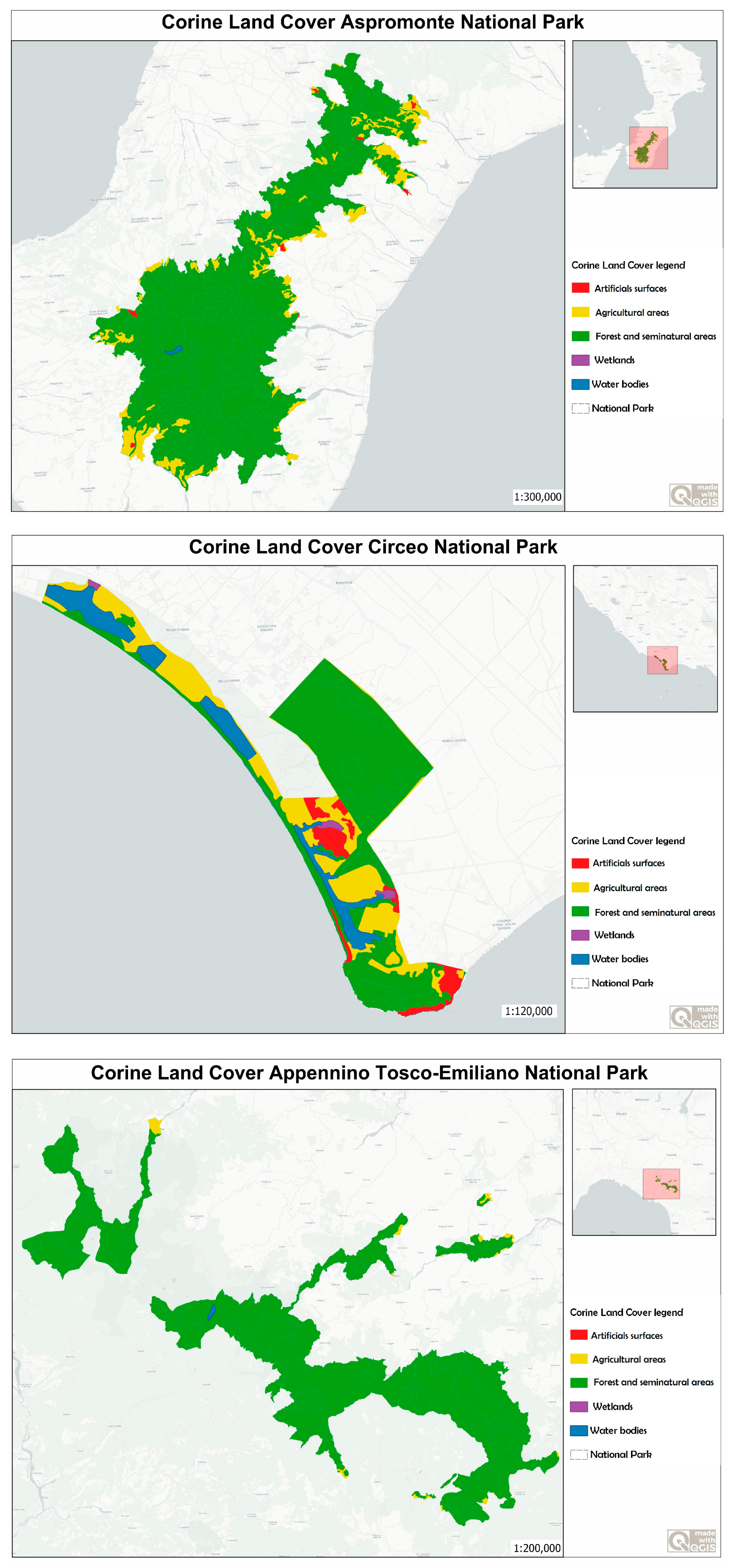
2.1. Case Studies

The framework illustrated in Figure 2 was applied to three national parks in Italy: the Appennino Tosco Emiliano National Park, the Circeo National Park, and the Aspromonte National Park. The choice of the three case studies fell on three areas distinguished by localization, environmental and socio-economic context (Table 1), and land use (Figure 1).
The Appennino Tosco Emiliano National Park extends along the ridge of the Apennines and is mainly characterized by a hilly-mountainous landscape. It is mainly characterized by wooded areas and semi-natural environments (Figure 1). The Circeo National Park, one of the first parks to be established in Italy (in 1934), develops mainly along the coastal stretch of the Tyrrhenian coast. In addition to the forest areas within the park, there are agricultural and artificial areas (Figure 1). The artificial areas include the urbanized center (i.e., the town of Sabaudia), the marina, and the accommodation facilities located along the coast.
Lastly, the Aspromonte National Park is characterized by wilderness/mountainous areas and agricultural areas mainly linked to agroforestry-pastoral activities (Figure 1).
The most important economic activities are the retail sector (ATECO class 47) and the agricultural sector (ATECO class 01) equating to 18.97% and 13.79% respectively of the number of companies in the area (Unioncamere, 2015). ATECO is a type of classification adopted by the Italian National Statistical Institute (ISTAT) for national statistical surveys of economic nature All three sites investigated conform to the “Plan of Park” (a legal strategy concerning protected natural, environmental, historical, cultural, and anthropological assets); in addition, the Aspromonte National Park also conforms to the Park regulation and Multi-year economic and social plan, as required by the Framework Law on Protected Areas 394/91.

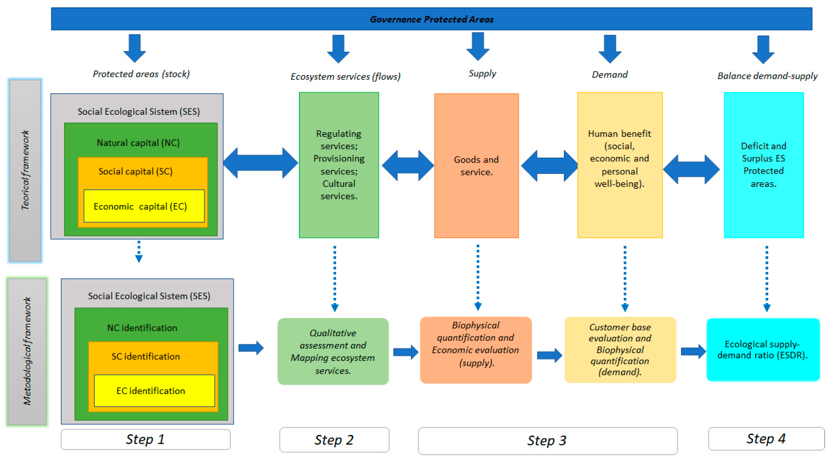
2.2. Theoretical and Methodological Framework

In this study, the analysis of the demand and supply of ES in protected areas is based on the framework shown in Figure 2. The framework consists of a theoretical part “theoretical framework” and of an application part “methodological framework”.
In the theoretical framework, the links between the various components are bidirectional as the change in the state of one component can affect the state of the others.
Within the Social-Ecological System (SES) of protected areas, NC generates ES (Figure 2) through its interaction with other forms of capital such as human, social, and built capital [7,53]. NC includes processes and functions which generate resources, later extracted by the economic system and transformed into goods and services and utilized by the social system in the various forms of traditional use. EC is largely the result of traditional economic activities and practices (The concept of traditional in this chapter refers primarily to the material culture (traditional knowledge) with which local populations have co-evolved with the natural and semi-natural environment, still evident in rural areas, particularly in the Mediterranean [55]), which are the result of a long co-evolutionary path, of anthropogenic adaptation and the transformation of specific ecosystems. The livelihood of local communities depends mainly on traditional economic activities and practices (agriculture, grazing, fishing, forestry, harvesting of non-wood products, etc.) which are typical of rural environments [53]. Accordingly, as in most protected areas, the landscape is the result of a long evolutionary process that has seen the interaction between humans and nature, and its utmost expression is illustrated by distinctive cultural and landscape features.
The goods and services provided by the NC are seen as public goods and therefore their benefits are very often not internalized in economic markets and thereby are excluded from public investments. It is, therefore, possible to ascribe a value of direct and indirect use to these goods and services. This value can be expressed in different forms using monetary, non-monetary, or qualitative criteria [5,8,56,57]. Hence the need to ascribe an economic value to these services and, at the same time, to understand consumption in order to implement a model of economic and sustainable growth in compliance with the ecological balances generated by ecosystems.
Consumption of ES, represented by demand, is closely related to the other components of the SES (Figure 2) [19]. Demand can be influenced by various factors, such as socio-economic conditions, demographic changes, and technological innovations [10]. Growth and changes in population composition can influence patterns of consumption or use, as well as individual preferences [19]. Furthermore, demand is also influenced by the individual needs of potential beneficiaries, their awareness, opportunities, and costs of using specific ES (e.g., access, availability) [14].
Our research considers the balance (deficit/surplus) between supply and demand with respect to a specific catchment area. The analysis of the budget in terms of deficit/surplus becomes important in an effort to redeploy governance processes for the protection of biodiversity both upstream, for better management of protected areas and therefore of the Social-Ecological System (stock), and on production models (flows) and consumption (demand) of natural resources by the SES.
The methodological approach (Figure 2), based on the acquisition of useful information to describe the stocks (the different forms of capital investigated) and the flows (the ES that originate from the latter), was developed in accordance with the theoretical approach (Figure 2). The methodological process follows a sequential and parallel approach to the theoretical one and includes; an understanding of the reference context through the analysis of stocks; the identification and quantification of ES; the estimation of benefits; the identification of beneficiaries in the catchment area and the balance between supply and demand obtained through the calculation of the ecological Supply-Demand ratio (ESDR).
Biophysical analysis is relevant for the assessment of capital stocks (natural, social, and economic), flows of ES (supply), and impacts on resources caused by consumption (demand). The economic valuation can affirm the importance of ES and assist communication with policy-makers responsible for the implementation of adaptive land management.

2.2.1. Step 1. Capital Identification

The first step identifies the different forms of capital for each protected area investigated, starting from the analysis of the area of reference. The NC includes ecosystems that do not require human intervention for their formation [47]. In this paper, natural capital is analyzed according to the community habitats identified by Directive 92/43/EEC. Each community habitat is able to provide more ES [57]. The establishment of these habitats in the European Union makes it possible to reduce the pressures on the environment from the Socio-Economic System, which can alter the supply of ES. Social capital (SC) constitutes the social networks and norms which facilitate cooperation, including human capital, culture, and institutions [48]; economic capital (EC) is the built capital produced by people, represented by final consumer goods or intermediate goods used for the production of other goods, and also financial capital. For the analysis of the SC and of the EC, we herein refer to data from statistical sources in order to investigate the territorial scope both in reference to economic activities and to public and private subjects which distinguish the community of the investigated areas.

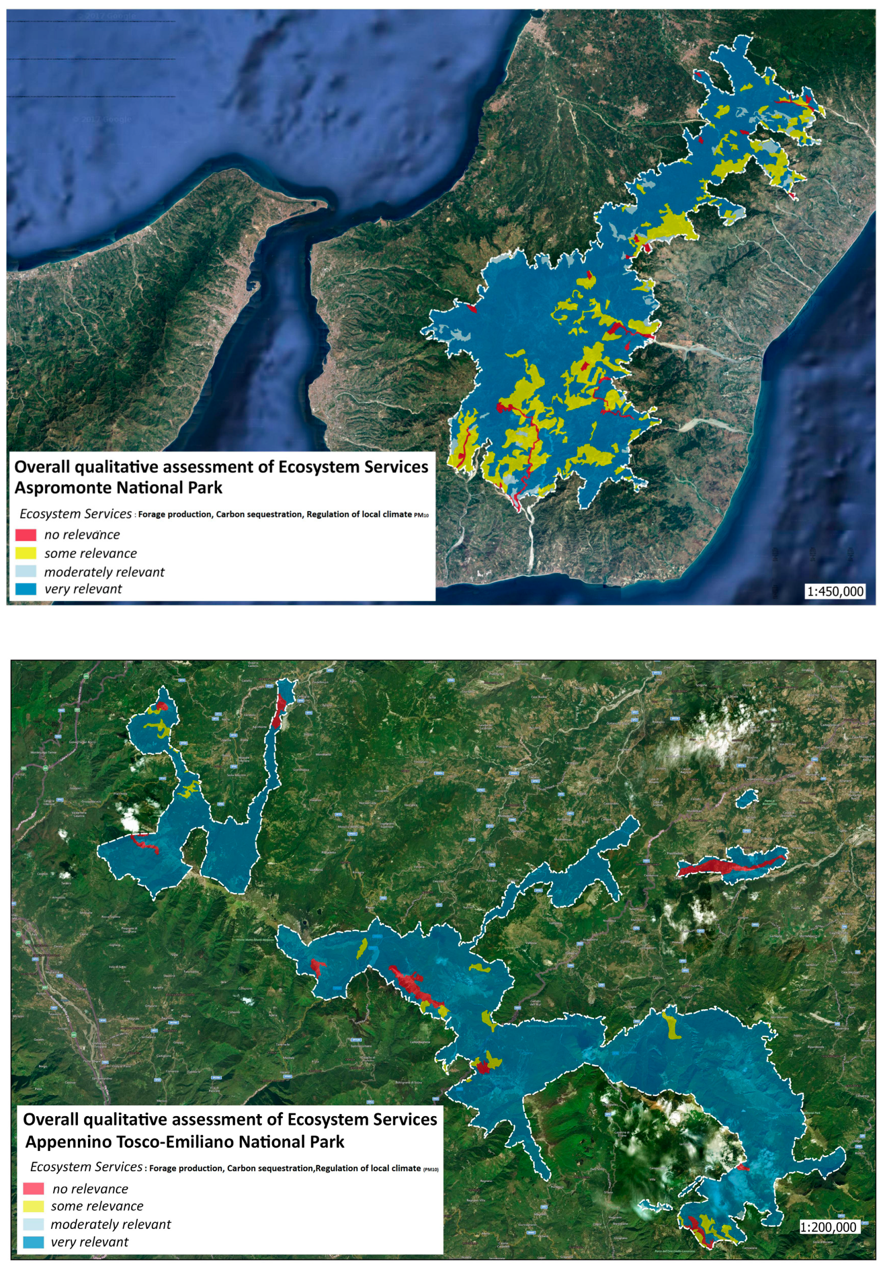
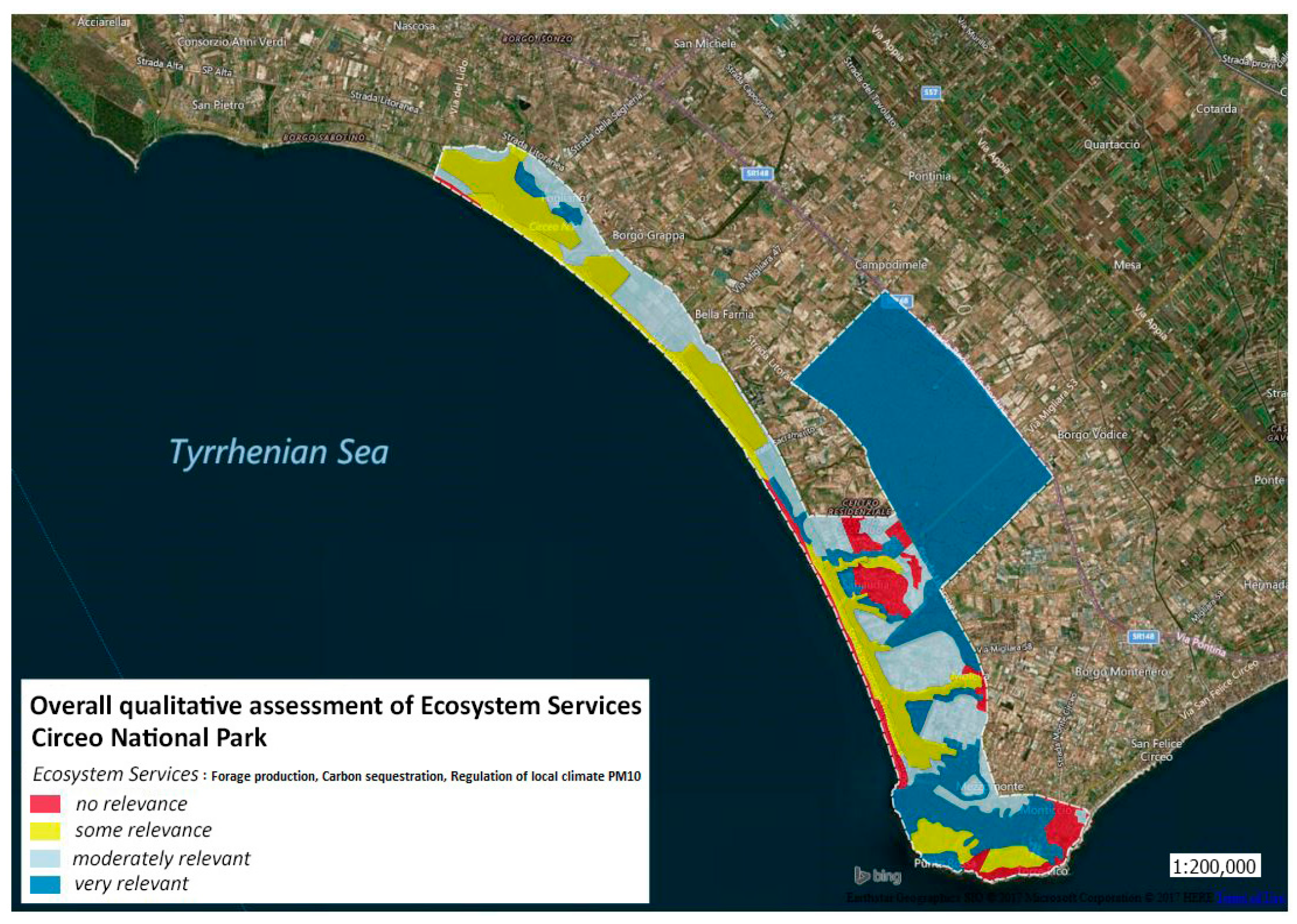
2.2.2. Step 2. Valuation and Mapping of ES

Mapping the areas that provide ES is an important aspect as it allows for the development of strategies that will ensure the supply of ES in the future [12]. According to De Vreesea et al. [58], the mapping of the most used ES supply in scientific studies is mainly based on land use and land cover and the spatial distribution of biophysical/abiotic resources and flows [59,60,61,62,63]. In this study, the mapping of the ES was based on land cover and use (Corine Land Cover, 2012), which allowed the identification of the most relevant ES for protected areas. For the qualitative assessment, each Corine Land Cover class was assigned a relevance class (3-very relevant, 2-moderately relevant, 1-with some relevance, 0-no significant relevance) which indicates the land use capacity to provide different SE [57]. The relevance classes were assigned by Schirpke on the basis of some parameters (density of function, potential distance from demand, intrinsic biodiversity). In our study, we used these relevant classes because the Circeo National Park, the Aspromonte National Park, and the Appennino Tosco Emiliano National Park include Natura 2000 sites with territorial characteristics and Community habitats (Directive 94/43/EEC) similar to those investigated by Schirpke [57]. The classification adopted for the ES is the one presented in the LIFE + MGN project (http://www.lifemgn-serviziecosistemici.eu/IT/Documents/doc_mgn/LIFE+MGN_Report_A2.4.pdf, accessed on 25 November 2020).

2.2.3. Step 3. Biophysical Quantification (Supply-Demand) and Economic Evaluation

The supply of ES is influenced by natural factors (habitat, fauna, flora, vegetation, latitude, altitude, etc.) as well as by anthropogenic factors: for example, the variation in land use and land cover affects the ability of ecosystems to provide goods and services and consequently of meeting the needs of society. Biophysical quantification methodologies of the supply may vary according to the type of ecosystem service being analyzed. For example, supply ES can be investigated through biophysical indicators (quantity of forage produced), cultural ES by taking into consideration a set of biophysical and social aspects, and lastly regulatory ES can be quantified through the analysis of ecosystem processes (e.g., carbon sequestration [10]). The indicators used to quantify supply must be sensitive to changes in land cover and land use at both spatial and temporal scales [64]. The demand for ES can be traced back to different scales [65] as it is functional to the very nature of ES. For example, the demand for carbon sequestration and climate regulation can be analyzed on a global scale, while forage production can be analyzed on a local scale [31]. In this paper, the analysis of the demand was carried out by identifying the potential consumers of ES within the area of impact of the benefits induced by the ES themselves. The catchment area includes municipalities with a minimum surface share of 45% within the investigated national parks [66], thereby focusing on the network of areas immediately gravitating around each park, rather than on the phenomena observed within the perimeter of the park.
The aim is to quantify the demand from potential consumers such as local communities, stakeholders, and economic activities (tourism, agriculture, livestock, commercial establishments, etc.), which benefit from the flow of goods and services generated by ecosystems. An economic valuation of the ES is important as it allows the ascription of a price to goods that are not traded on the market. Ignoring the economic value of a resource can lead to the damage and impoverishment of ES. The economic valuation of the ES supply takes place through monetary techniques belonging to both traditional valuation and consumer surplus (preferences expressed and detected) [67]. The choice of the most appropriate economic technique depends on biophysical quantification which makes it possible to define the economic features ((non) rival and (non) excludable) of the investigated ES. Moreover, as highlighted by various studies [68,69] the attribution of the values of use and non-use of the ES must be carried out through an interdisciplinary approach, which takes into account, in addition to the biophysical analysis, the spatial scale of reference, the perception of the benefits by the local community correlated to territorial dynamics, as well as from the institutional context of reference. The present study utilized methods of economic valuation which belong to the market price and to the avoided costs selected according to the ES analyzed.

Forage Production

The average productivity values of forage available at the regional level were used for the biophysical quantification of supply ES [70]. These values were multiplied by the
Extension of grassland and pastures for each protected area, thus obtaining the average productivity values.
Supply = Average regional forage production (t/ha) * national park grassland and pastures area (ha).
The economic valuation was carried out taking into consideration the forage price in Italy (between 100 and 150 euro per tonne) multiplied by the average production of each site.
Economic value = average forage production (t) * average market price (€/t).
The ES demand was evaluated considering the average consumption per capita by type of livestock within the catchment area.
Demand = average consumption of forage per capita (t/year/head) * head of cattle/sheep/buffalo (n. of heads).

Carbon Sequestration

The biophysical quantification of carbon sequestration can be carried out by estimating stored carbon in the wood mass (carbon stock) and/or processed (carbon sink). In this study the quantity of carbon processed was estimated considering the epigeal component of the forests, taking into account the increment as a function of the arboreal phytomass of each forest type, as distinguished by region. Phytomass is converted into carbon at a general carbon/phytomass ratio (0.5) and a fresh weight/dry weight ratio which varies according to the forest type. The dataset took into account the National Inventory of Forests and Forest Reservoirs of Carbon Forests INFC (Forestry National Inventory on Carbon Reservoirs) in Italy.
The formula used to measure supply is the following:
Supply (tC/year (site-s, region-s)) = Incr × BEF × WBD × 0.5.
where:
Incr =
Current increment in epigeal tree volume per hectare, by region, and by forest type [Table A1].
BEF =
BEF conversion factor (epigeal biomass/growing stock, Biomass Expansion Factor).
WBD =
basal density of wood dry weight/fresh weight (t/m3) (Table A2).
There are two approaches for the economic valuation of ES carbon sequestration: one is based on the Social Cost of Carbon (SCC), and the other on the market value of emission permits. Specifically, the social cost takes into account the damage avoided, at a global level, through the sequestration of CO2. This calculation is rather mutable as both value and price per tonne of carbon are subject to considerable fluctuations on the international market. For example, different estimates have led to very heterogeneous values: between 32 $ tC and 326 $ tC. [71]. Otherwise, the market value is the price established by the market for emission permits, and according to the European Climate Exchange, the price ranged from 153 $ tC in 2008 to 12 $ tC in 2012. In this paper, the social cost, in reference to the value estimated by Ricke and colleagues [72] of 417 $/t CO2 (approx 374.89 €/t CO2), as well as the price of a tonne of carbon on the emission allowance market were considered (https://ember-climate.org/data/carbon-price-viewer/ accessed on 31 December 2018). These values were multiplied by the equivalent tonnes of CO2 captured by each of the parks investigated.
Economic value (€) = CO2 captured by forest biomass (t/year) * social cost (€/t).
Economic value (€) = CO2 captured by forest biomass (t/year) * market price (€/t).
The demand for CO2 storage was assessed with reference to local anthropogenic emissions, taking into account the number of employees of economic enterprises in the catchment area. The type and number of economic enterprises in the catchment area were identified and provided by Unioncamere (Italian Union of Chambers of Commerce, Industry, Crafts and Agriculture). The Italian Statistical Institute (ISTAT) classifies economic enterprises into the ATECO categories (i.e., economic activities), recording the total number of employees per enterprise. To estimate the CO2 emissions of each enterprise the ATECO categories have been reclassified into a macro category known as Selected Nomenclature for Air Pollution (SNAP 97) (The SNAP 97 classification (Selected Nomenclature for Air Pollution), which identifies 11 macrosectors of pollutant emissions, was defined within the Corine air project, promoted and coordinated by the European Community DG XI as part of the Corine experimental program (Coordinated Information on the Environment in the European Community), undertaken by the Commission of the European Communities following the decision of the Council of 27 June 1985. Each SNAP 97 category is also reclassified within the respective emission sources established by the IPCC). The process of reclassification was complex as it was not always possible to find a direct correspondence between the ATECO categories and the macro sectors of polluting activities into which the SNAP 97 classification is divided. Reclassification made it possible to estimate the CO2 demand in the catchment area of each national park investigated, according to the number of employees per economic enterprise. Estimates of carbon emissions by the energy services sector only concern the combustion of non-renewable energy sources.
Demand (tCO2) = CO2 emissions (t/no. of employees per economic enterprise) * employees per economic activity national park (n).

Regulation of Local Climate (PM10)

The ES supply was based on the ability of protected areas to capture PM10 particles (<10 μm). The amount of PM10 in the atmosphere is influenced both by the vegetation present in an area and by rainfall and temperatures [73,74].
The annual capture coefficients of PM10—by type of vegetation extrapolated from the scientific literature—were used to calculate supply [75,76,77] and assigned according to the Corine Land Cover classification (Table A3). The formula used to calculate the ES supply is the following:
Supply = capture coefficients by type of forest (t/ha/year) * type of forest (ha).
A rough estimate of the capture potential of PM10 is obtained by multiplying the surfaces of each Corine Land Cover cover of the national parks investigated by the relative capture coefficient.
The monetary value was calculated by taking into account the avoided costs (social damage) as a result of the capture function of PM10 by plants, which is equal to €5484.61 for each tonne of PM10 absorbed [78] (converted from 2008 to 2018 € value).
Economic value (€) = PM10 captured (t/year) * social cost (€/t).
The calculation of PM10 demand is complex as it requires precise data on emissions (from environmental monitoring) or potential emissions by surface category or production activities (factories, roads, agriculture, etc.). In order to overcome the difficulties in obtaining data or lack thereof, we estimated PM10 emissions relating to employees by following the same methodology used to estimate the demand for carbon absorption. Therefore, having reclassified the ATECO classes in SNAP 97 categories and calculated the relative PM10 emissions per employee at the national level, the latter was multiplied by the number of employees per service area. PM10 emissions at the national level were calculated by dividing the PM10 emissions of the individual SNAP 97 classes by the relative total number of employees.
The formula used to measure demand is as follows:
Demand (tonnes PM10) = PM10 emissions (t/n employees in economic enterprise)* employees in economic enterprise (n.).

2.2.4. Balance Demand-Supply

The ecological supply-demand ratio (ESDR) was calculated from the biophysical data obtained through the application of the methodological procedure. In the bibliography, this indicator is mainly used for a space-time comparison of site-specific supply and demand [34]. In this study, the balance between supply and demand focused instead on a spatial comparison to verify the state of ES in the areas investigated. For this purpose, the actual supply and the effective demand calculated for each ecosystem service in each park area were compared using the following equations (modified from Chen [34]):
ESDR = s u p p l y   a c t u a l   E S     d e m a n d   E S ( s u p p l y a c t u a l E S   + d e m a n d   E S ) / 2
where supply actual ES represents the biophysical supply of each ecosystem service investigated in the study areas and demand ES the consumption of ES by potential resident consumers in the catchment area. Values above zero represent a surplus of ES, whereas < zero represents a deficit and equal to zero a balance between supply and demand [32].

3. Results

For each protected area, the contribution of NC, SC, and CE to the supply of ES was identified [53] (Table 2). As Table 2 illustrates, the three national parks investigated show an evident heterogeneity of Natura 2000 habitats which testifies to the biodiversity richness at the community level. Conversely, the social and economic fabric presents some differences between the parks. The Aspromonte National Park and the Appennino Tosco Emiliano National Park, being predominantly rural areas, have similar SC and NC. What sets them apart is the variety of products grown, processed, and marketed in relation to the peculiarities of the territory. The Circeo National Park is a coastal park and its SC and EC are linked to seaside tourism and to the production and processing of wine and oil products. Public human capital depends on the political-administrative division of the Italian territory.
Figure 3 shows the qualitative mapping of ES in the studied areas. Most of the territories of the Appennino Tosco Emiliano National Park and the Aspromonte National Park provide ES that are very relevant to society. This result is mainly due to the coverage of forest and vegetation and to the reduced surface of urbanized areas. In fact, if on the one hand urbanized areas do not provide SE, on the other hand, the forest areas perform relevant functions including climate change mitigation (carbon sequestration) and air purification (PM10) on a local scale. The two parks constitute territories with a significant supply of ES and low demand.
The Circeo National Park is also characterized by artificial areas dislocated along the coast. The areas that provide the most SE are the Circeo Promontory, the Circeo state forest (Biosphere reserve Man and the Biosphere – MAB Programm), and water bodies and wetlands near the coastal dunes (very relevant areas Figure 3). From the spatialization of the demand (Figure 4) it is evident that the potential catchment area of the analyzed ES corresponds to densely populated areas and agricultural areas. The data of biophysical quantification of supply and demand and economic value by ES are shown in Table 3.
As Figure 5 shows, the ESDR of ES is not always positive. This depends on the one hand on the capacity of the land to provide ES (supply) and on the other on the economic and social fabric that distinguishes the catchment area (demand). The Circeo National Park shows a deficit in the ES of forage production and regulation of local climate (PM10) (Figure 5). The negative ESDR values for the forage production ES are due to a reduced cover of the grassland and pasture areas used for forage production. The production of forage (5250 t) does not satisfy the demand (25,282 t). As for the ES regulation of local climate (PM10), the results also show that compared to PM10 emission into the atmosphere of approximately 13,518 t/year, only 65.30 t/year PM10 is deducted by the forest constituent. For the Aspromonte National Park as well, the spatial comparison of demand and supply of the ES forage production shows a deficit. Despite 4.6% of the territory being allocated to grazing (Table 1), it fails to meet the demand of approximately 46,930 t of forage per year required by 36,681 heads of cattle (bovine, buffalo, goat, sheep). Conversely, the relationship between supply and demand for the carbon sequestration ES is positive, which is a common trend for the investigated parks. This highlights the importance of the contribution made by forest cover to the mitigation of climate change on a local scale.
The ESDR calculated at the system level of the protected areas investigated (Figure 6) acquire positive values for all three ES. This highlights how, overall, the benefits of establishing protected areas are linked to the protection of the supply areas of ES. The supply balances the demand not only at the catchment level but also at a regional and global scale. As the investigated ES have a higher value than 1328 billion euro, the estimated benefits (Table 3) are higher than management costs: for each euro invested there is a return of around 228 euro.

4. Discussion

Studies with a focus similar to ours have found it challenging to deal with the different scales between social and ecological systems. In fact, socio-economic data are usually made available on administrative surveys and it is necessary to georeference them so as to relate them to the scale of the survey [79,80]. In addition, many ES (support services, nutrient cycle, etc.) are absent from the market. They require indirect methods, such as avoided cost, to be economically quantified. Our research used two estimation methodologies, one based on the market price to value the ES of forage production and the other based on social costs for the regulatory ES intrinsic to carbon sequestration and the regulation of local climate (PM10).
The results reported in this study consider the need to improve the conservation of natural capital by taking into account the spatial relationship between the supply and demand of ES. Improving the understanding of the relationship between supply and demand of services in different areas is recognized as a fundamental aspect that must take into account the ES framework [81].
The analysis, conducted through the use of ESDR, is important as it provides an opportunity to understand the socio-economic context (for example ATECO economic activity) that can change the ability of NC to provide ES.
The ESDR index has highlighted a different contribution made by national parks to the provision of ES, in response to social and economic demand. The ESDR index shows, to varying degrees, that the Circeo National Park is unable to compensate for the CO2 emissions from anthropogenic activities. The results reveal the need to undertake a policy of conversion of energy policies aimed at reducing emissions at the local and global levels.
There is also an imbalance between the supply and demand of fodder for the Circeo National Park as the agricultural areas are mainly used for the cultivation of vines and olive groves (Table 3).
Air pollution due to PM10 represents one of the main health risks for citizens. In our study, the ESDR value is positive in the three parks analyzed (Figure 5). This is due not only to the ability of the forest component to absorb PM10 but also to the characteristics of the socio-economic context. The ESDR shows that the parks are able to absorb part of the PM10 emitted by economic activities also present in the neighboring areas (catchment area). The capture of PM10 by vegetation can produce economic benefits such as, for example, the reduction of health costs related to air pollution.
The economic benefit of the three parks relative to the social costs avoided thanks to the capture of PM10 is approximately 973 million euros. If we add up the avoided costs due to carbon sequestration, the total economic benefit is 1290 billion euro.
Therefore, an effective assessment of ES requires an analysis of the actual needs of society in relation to the supply of services and their ability to reach the areas of demand through service flows [82].
This paper highlights how the flow of goods and services depends on the synergy of the environmental, social, and economic capital while the demand depends on the economic activities falling within the catchment area.
To calculate supply and demand it is necessary to analyze the social and economic drivers [83] responsible for inducing variations in the flow of goods and services [84]. It is important to understand the spatial relationships among the areas in which ES originate (supply) and those that benefit from them (demand), correlating the calculation of supply and demand to the reference scale, in order to implement effective policies [85,86].
Furthermore, the ecological and economic processes from which the different ES emerge and the utility flows may not match their point of origin [49,86,87].
For example, the place of ES forage production and the benefitting areas can be in situ (Services Providing Units (SPU) and Services Benefiting Areas (SBA) are realized in the same location) and decoupled from the point of supply as these goods/services can also be exchanged over long distances [31]. The benefitting areas of the ES carbon sequestration and ES regulation of local climate (PM10) are localized not only at the point of origin (in situ) but also in an omnidirectional way, as the benefit expands from the point of production (SPU in one location, SBA in the surrounding landscape without directional bias) [31]. Adequate levels of governance of park areas would guarantee the continuous flow of goods and services by limiting the externalities of the production and consumption of resources at the system level [44]. Taking the work of Burkhard et al. [31], and Kettunen [88] as reference, the benefits (ES) provided by the three protected areas can be felt at different scales (Table 4).
The benefits provided by regulation ES such as carbon sequestration and regulation of local climate (PM10) exceed the boundaries of the protected area and reach society as a whole, while the benefits deriving from the ES supply of forage and grazing mainly concern the local scale.

5. Conclusions

The objective of the present paper was to evaluate the application of a method for calculating the flows of ES which would highlight, on a physical-spatial, social and political basis, the relationships established between the areas in which such flows originate and the areas that benefit from them. Specifically, the supply areas investigated were three Italian national parks and the beneficiaries were the respective areas from which the demand for three indicative ES originates.
Ultimately, through the mapping of supply and demand of ES, studies such as this one provide an opportunity to identify the economic value of the services themselves, and also to map the different stakeholders and their roles, facilitating the identification of management tools (regulatory, planning or market-based tools such as payments for ES) aimed at preserving natural capital, maintaining the flow of ES, and therefore social welfare. In this context, the application of the ES supply and demand ratio (ESDR) can potentially improve the application of management tools. In the event of a surplus in the supply, it is, in fact, possible to identify ex-ante the service use limit, or alternatively, policies aimed at increasing conservation and natural capital to increase supply levels, in order to avoid the over-exploitation of resources.

Author Contributions

Conceptualization, M.P., D.M., and A.M.; methodology, M.P., D.M., and A.M.; formal analysis, M.P., M.T., and A.M.; data curation, M.T., M.P.; writing—original draft preparation, M.P., A.M., and D.M., writing—review and editing, M.P., A.M. All authors have read and agreed to the published version of the manuscript.

Funding

Research funds: Unioncamere.

Institutional Review Board Statement

Not applicable.

Informed Consent Statement

Not applicable.

Data Availability Statement

The data presented in this study are available on request from the corresponding author.

Acknowledgments

We thank Unioncamere for providing some data.

Conflicts of Interest

The authors declare no conflict of interest.

Appendix A

Table A1. Values per unit of surface area of the epigeal arboreal phytomass for the forest categories of high woods (m3/ha) [75].
INFC CategoriesRegions
Emilia
Romagna
ToscanaLazioCalabria
Spruce woods13.213.320.20
white spruce woods12.412.308.6
Scots pine and Mountain pine3.98.700
Black pine forests, laricio pine forests6.38.75.58.6
Mediterranean pines4.34.23.44.7
Other coniferous forests, pure or mixed4.87.88.310.3
Beech woods6.28.13.56.4
Oak wood, Downy Oak Woods, English oak woods2.21.91.52.3
Sessile oak and other oaks4.72.93.14.8
Chestnut groves5.36.46.66.2
Hornbeams3.23.82.21.8
Hygrophilous woods3.44.63.34.5
Other deciduous forests3.44.32.73.4
Holm oak woods5.22.31.93.7
Cork oak woods02.32.12.7
Others broadleaves02.11.13
Table A2. Biomass expansion factor (BEF) and basal density of wood (WBD) values [75].
INFC CategoriesWBDBEF
Spruce woods0.381.29
white spruce woods0.381.34
larch woods and stone pine woods0.561.22
Scots pine and Mountain pine0.471.33
Mediterranean pines0.531.53
Other coniferous forests, pure or mixed0.431.37
Beech woods0.611.36
Sessile oak and other oaks0.691.45
Chestnut groves0.491.33
Hornbeams0.661.28
Oak wood, Downy Oak Woods, English oak woods0.651.39
Holm oak woods0.721.45
Cork oak woods0.721.45
Other deciduous forests0.531.47
Black pine forests, laricio pine forests0.521.44
Hygrophilous woods0.411.39
Others broadleaves0.631.49
Table A3. PM10 sequestration coefficients for Corine Land Cover class (III level) [75].
Corine Land Cover ClassCoefficient *Approach
3.1.1. Broad-leaved forest0.16 t/ha/yeardata 1/3 of the value for coniferous
3.1.2. Coniferous forest0.49 t/ha/yearaverage approx. of the highest values of Escobedo and Nowak [76], Nowak et al. 2006 [77], compared to fully wooded areas (x 4)
3.1.3. Mixed forest0.325 t/ha/yearaverage of the previous values
* The coefficients do not consider the contribution of shrubs and grassy surfaces.

References

  1. MEA. Ecosystems and Human Well-Being: Biodiversity Synthesis; World Resource Institute: Washington, DC, USA, 2005. [Google Scholar]
  2. Wu, S.; Li, S. Ecosystem service relationships: Formation and recommended approaches from a systematic review. Ecol. Indic. 2019, 99, 1–11. [Google Scholar] [CrossRef]
  3. Graeme, S.C.; von Cramon-Taubadel, S. Linking economic growth pathways and environmental sustainability by understanding development as alternate social–ecological regimes. Proc. Natl. Acad. Sci. USA 2018, 115, 9533–9538. [Google Scholar]
  4. Wang, Z.; Mao, D.; Li, L.; Jia, M.; Dong, Z.; Miao, Z.; Ren, C.; Song, C. Quantifying changes in multiple ecosystem services during 1992–2012 in the Sanjiang Plain of China Sci. Total Environ. 2015, 514, 119–130. [Google Scholar] [CrossRef]
  5. Haines-Young, R.; Potschin, M. The links between biodiversity, ecosystem services and human well-being. Ecosyst. Ecol. New Synth. 2010, 1, 110–139. [Google Scholar]
  6. Burkhard, B.; Kroll, A.; Nedkov, S.; Müller, F. Mapping ecosystem service supply, demand and budgets. Ecol. Indic. 2012, 21, 17–29. [Google Scholar] [CrossRef]
  7. Costanza, R.; de Groot, R.; Sutton, P.C.; van der Ploeg, S.; Anderson, S.; Kubiszewski, I.; Farber, S.; Turner, R.K. Changes in the global value of ecosystem services. Glob. Environ. Chang. 2014, 26, 152–158. [Google Scholar] [CrossRef]
  8. Burkhard, B.; Maes, J. Mapping Ecosystem Services; Pensoft Publishers: Sofia, Bulgaria, 2017; 374p, Available online: http://ab.pensoft.net/articles.php?id=12837 (accessed on 21 November 2020).
  9. Wei, H.; Fan, W.; Wang, X.; Lu, N.; Dong, X.; Zhao, Y.; Ya, X.; Zhao, Y. Integrating supply and social demand in ecosystem services assessment: A review. Ecosyst. Serv. 2017, 25, 15–27. [Google Scholar] [CrossRef]
  10. Villamagna, A.M.; Angermeier, P.L.; Bennet, E.M. Capacity, pressure, demand, and flow: A conceptual framework for analyzing ecosystem service provision and delivery. Ecol. Complex. 2013, 15, 114–121. [Google Scholar] [CrossRef]
  11. Crossman, N.D.; Burkhard, B.; Nedkov, S.; Willemen, L.; Petz, K.; Palomo, I.; Drakou, E.G.; Martín López, B.; McPhearson, T.; Boyanova, K.; et al. A blue print for mapping and modeling ecosystem services. Ecosyst. Serv. 2013, 4, 4–14. [Google Scholar] [CrossRef]
  12. Martínez-Harms, M.J.; Balvanera, P. Methods for mapping ecosystem service supply: A review. Int. J. Biodivers. Sci. Ecosyst. Serv. Manag. 2012, 8, 17–25. [Google Scholar] [CrossRef]
  13. Bastian, O. The role of biodiversity in supporting ecosystem services in Natura 2000 sites. Ecol. Indic. 2013, 24, 12–22. [Google Scholar] [CrossRef]
  14. Schröter, M.; Barton, D.N.; Remme, R.P.; Hein, L. Accounting for capacity and flow of ecosystem services: A conceptual model and a case study for Telemark, Norway. Ecol. Indic. 2014, 36, 539–551. [Google Scholar] [CrossRef]
  15. Richards, D.R.; Friess, D.A. A rapid indicator of cultural ecosystem service usage at a fine spatial scale: Content analysis of social media photographs. Ecol. Ind. 2015, 53, 187–195. [Google Scholar] [CrossRef]
  16. Egoh, B.N.; Paracchini, M.L.; Zulian, G.; Schägner, J.P.; Bidoglio, G. Exploring restoration options for habitats, species and ecosystem services in the European Union. J. Appl. Ecol. 2014, 51, 899–908. [Google Scholar] [CrossRef] [Green Version]
  17. Stürck, J.; Poortinga, A.; Verburg, P.H. Mapping ecosystem services: The supply and demand of flood regulation services in Europe. Ecol. Indic. 2014, 38, 198–211. [Google Scholar] [CrossRef]
  18. Larondelle, N.; Lauff, S. Balancing demand and supply of multiple urban ecosystem services on different spatial scales. Ecosyst. Serv. 2016, 22, 18–31. [Google Scholar] [CrossRef]
  19. Wolff, S.; Schulp, C.J.E.; Kastner, T.; Verburg, P.H. Quantifying spatial variation in ecosystem services demand: A global mapping approach. Ecol. Econ. 2017, 136, 14–29. [Google Scholar] [CrossRef]
  20. Nikodinoska, N.; Paletto, A.; Pastorella, F.; Granvik, M.; Franzese, P.P. Assessing, valuing and mapping ecosystem services at city level: The case of Uppsala (Sweden). Ecol. Mode 2018, 368, 411–424. [Google Scholar] [CrossRef]
  21. Balvanera, P.; Quijas, S.; Karp, D.S.; Ash, N.; Bennett, E.M.; Boumans, R.; Brown, C.; Chan, K.M.A. Ecosystem services. In The GEO Handbook on Biodiversity Observation Networks; Walters, M., Scholes, R.J., Eds.; Springer Open: Cham, Switzerland, 2016; pp. 39–78. [Google Scholar]
  22. Yahdjian, L.; Sala, O.E.; Havstad, K.M. Rangeland ecosystem services: Shifting focus from supply to reconciling supply and demand. Front. Ecol. Environ. 2015, 13, 44–51. [Google Scholar] [CrossRef]
  23. Lamarque, P.; Quétier, F.; Lavorel, S. The diversity of the ecosystem services concept and its implications for their assessment and management. CR Biol. 2011, 334, 441–449. [Google Scholar] [CrossRef]
  24. Honey-Rosés, J.; Pendleton, L.H. A emand Driven Research Agenda for Ecosystem Services. Ecosyst. Serv. 2016, 1, 160–162. [Google Scholar]
  25. Balvanera, P.; Daily, G.C.; Ehrlich, P.R.; Ricketts, T.H.; Bailey, S.A.; Kark, S.; Kremen, C.; Pereira, H. Conserving biodiversity and ecosystem services. Science 2001, 291, 2047. [Google Scholar] [CrossRef] [PubMed]
  26. Vollmer, D.; Shaad, K.; Souter, N.J.; Farrell, T.; Dudgeon, D.; Sullivan, C.A.; Fauconnier, I.; MacDonald, G.M.; McCartney, M.P.; Power, A.G.; et al. Integrating the social, hydrological and ecological dimensions of freshwater health: The Freshwater Health Index. Sci. Total Environ. 2018, 627, 304–313. [Google Scholar] [CrossRef]
  27. Feng, Z.; Cuib, Y.; Zhangc, H.; Gaoc, Y. Assessment of human consumption of ecosystem services in China from 2000 to 2014 based on an ecosystem service footprint model. Ecol. Indic. 2018, 94, 468–481. [Google Scholar] [CrossRef]
  28. Martínez-López, J.; Bagstad, K.; Balbi, S.; Magrach, A.; Voigt, B.; Athanasiadis, I.; Pascual, M.; Willcock, S.; Villa, F. Towards globally customizable ecosystem service models. Sci. Total Environ. 2019, 650, 2325–2336. [Google Scholar] [CrossRef] [PubMed]
  29. Bukvareva, E.; Zamolodchikov, D.; Kraev, G.; Grunewald, K.; Narykov, A. Supplied, demanded and consumed ecosystem services: Prospects for national assessment in Russia. Ecol. Indic. 2017, 78, 351–360. [Google Scholar] [CrossRef]
  30. Nedkov, S.; Burkhard, B. Flood regulating ecosystem services-mapping supply and demand, in the Etropole municipality. Bulgaria. Ecol. Indic. 2012, 21, 67–79. [Google Scholar] [CrossRef]
  31. Burkhard, B.; Kandziora, M.; Hou, Y.; Müller, F. Ecosystem Service Potentials, Flows and Demands—Concepts for Spatial Localisation, Indication and Quantification. Landsc. Online 2014, 34, 1–32. [Google Scholar] [CrossRef]
  32. Li, J.; Jiang, H.; Bai, Y.; Alatalo, J.M.; Li, X.; Jiang, H. Indicators for spatial–temporal comparisons of ecosystem service status between regions: A case study of the Taihu river basin, China. Ecol. Indic. 2016, 60, 1008–1016. [Google Scholar] [CrossRef]
  33. Guan, Q.; Hao, J.; Ren, G.; Li, M.; Chen, A.; Duan, W.; Chen, H. Ecological indexes for the analysis of the spatial–temporal characteristics of ecosystem service supply and demand: A case study of the major grain-producing regions in Quzhou, China. Ecol. Indic. 2020, 108, 105748. [Google Scholar] [CrossRef]
  34. Chen, J.; Jiang, B.; Bai, Y.; Xib Xu, X.; Alatalo, J.M. Quantifying ecosystem services supply and demand shortfalls and mismatches for management optimization. Sci. Total Environ. 2019, 650, 1426–1439. [Google Scholar] [CrossRef] [PubMed]
  35. Syrbe, R.U.; Grunewald, K. Ecosystem service supply and demand—The challenge to balance spatial mismatches. Int. J. Biodivers. Sci. Ecosyst. Serv. Manag. 2017, 13, 148–161. [Google Scholar] [CrossRef] [Green Version]
  36. Kroll, F.; Müller, F.; Haase, D.; Fohrer, N. Rural-urban gradient analysis of ecosystem services supply and demand dynamics. Land Use Policy 2012, 29, 521–535. [Google Scholar] [CrossRef]
  37. Guarini, M.R.; Morano, P.; Sica, F. Historical School Buildings. A Multi-Criteria Approach for Urban Sustainable Projects. Sustainability 2020, 12, 1076. [Google Scholar] [CrossRef] [Green Version]
  38. Cortinovis, C.; Geneletti, D. A performancebased planning approach integrating supply and demand of urban ecosystem services. Landsc. Urban Plan. 2020, 201, 103842. [Google Scholar] [CrossRef]
  39. Hummel, C.; Provenzale, A.; van der Meer, J.; Wijnhoven, S.; Nolte, A.; Poursanidis, D. Ecosystem services in European protected areas: Ambiguity in the views of scientists and managers? PLoS ONE 2017, 12, e0187143. [Google Scholar] [CrossRef] [Green Version]
  40. Tittensor, D.P.; Walpole, M.; Hill, S.L.; Boyce, D.G.; Britten, G.L.; Burgess, N.D. A mid-term analysis of progress toward international biodiversity targets. Science 2014, 346, 241–244. [Google Scholar] [CrossRef] [PubMed]
  41. Vitousek, P.M.; Mooney, H.A.; Lubchenco, J.; Melillo, J.M. Human domination of Earth’s ecosystems. Science 1997, 277, 494–499. [Google Scholar] [CrossRef] [Green Version]
  42. Sil, Â.; Rodrigues, A.P.; Carvalho-Santos, C.; Nunes, J.P.; Honrado, J.; Alonso, J. Trade-offs and synergies between provisioning and regulating ecosystem services in a mountain area in Portugal affected by landscape change. Mount. Res. Dev. 2016, 36, 452–464. [Google Scholar] [CrossRef] [Green Version]
  43. Buonocore, E.; Appolloni, L.; Russo, G.F.; Franzese, P.P. Assessing natural capital value in marine ecosystems through an environmental accounting model: A case study in Southern Italy. Ecol. Model. 2020, 419, 108958. [Google Scholar] [CrossRef]
  44. Marino, D.; Marucci, A.; Palmieri, M.; Gaglioppa, P. Monitoring the Convention on Biological Diversity (CBD) Framework using Evaluation of Effectiveness methods. The Italian case. Ecol. Indic. 2015, 55, 172–182. [Google Scholar] [CrossRef]
  45. Marino, D.; Gaglioppa, P.; Schirpke, U.; Guadagno, R.; Marucci, A.; Palmieri, M.; Pellegrino, D.; Gusmerotti, N. Assessment and governance of Ecosystem Services for improving management effectiveness of Natura 2000 sites. Biobased Appl. Econ. 2014, 3, 229–247. [Google Scholar]
  46. Marino, D.; Schirpke, U.; Gaglioppa, P.; Guadagno, R.; Marucci, A.; Palmieri, M.; Pellegrino, D.; De Marco, C.; Scolozzi, R. Assessment and Governance of Ecosystem Services: First insights from LIFE+ Making Good Natura project. Annali di Botanica 2014, 4, 83–90. [Google Scholar]
  47. Costanza, R.; Daly, H. Natural capital and sustainable development. Conserv. Biol. 1992, 6, 37–46. [Google Scholar] [CrossRef]
  48. Putnam, R.D. Tuning in, tuning out: The strange disappearance of social capital in America. Polit. Sci. Polit. 1995, 28, 664–683. [Google Scholar] [CrossRef]
  49. Fisher, B.; Turner, R.K.; Morling, P. Defining and classifying ecosystem services for decision making. Ecol. Econ. 2009, 68, 643–653. [Google Scholar] [CrossRef] [Green Version]
  50. Figueroa, E.; Aronson, J. New linkages for protected areas: Making them worth conserving and restoring. J. Nat. Conserv. 2006, 14, 225–232. [Google Scholar] [CrossRef]
  51. Carpenter, S.R. Alternate states of ecosystems: Evidence andits implications. In Ecology Achievement and Challenge; Huntly, M.C., Levin, S.N., Eds.; Blackwell: London, UK, 2001. [Google Scholar]
  52. Turner, R.A.; Addison, J.; Arias, A.; Bergseth, B.J.; Marshall, N.A.; Morrison, T.H.; Tobin, R.C. Trust, confidence, and equity affect the legitimacy of natural resource governance. Ecol. Soc. 2016, 21, 18. [Google Scholar] [CrossRef] [Green Version]
  53. Marino, D.; Palmieri, M. Investing in nature: Working with public expenditure and private payments for a new governance model. In Re-connecting Natural and Cultural Capital Contributions from Science and Policy; Paracchini, M.L., Zingari, P.C., Blasi, C., Eds.; Office of Publications of the European Union: Luxembourg, 2016. [Google Scholar]
  54. Schirpke, U.; Marino, D.; Marucci, A.; Palmieri, M.; Scolozzi, R. Operationalizing ecosystem services for effective management of protected areas: Experiences and challenges. Ecosyst. Serv. 2017, 28, 105–114. [Google Scholar] [CrossRef]
  55. Marino, D.; Cavallo, A. Understanding changing in traditional agricultural landscapes: Towards a framework. J. Agric. Sci. Technol. 2012, 2, 971–987. [Google Scholar]
  56. Ruskule, A.; Vinogradovs, I.; Pecina, M.V. The Guidebook on the Introduction to the Ecosystem Service Framework and Its Application in Integrated Planning; The LIFE Viva Grass project; University of Latvia: Rīga, Latvia, 2018; ISBN 978-9934-556-39-5. [Google Scholar]
  57. Schirpke, U.; Scolozzi, R.; De Marco, C. Analisi dei Servizi Ecosistemici Nei Siti Pilota. Parte 4: Selezione dei Servizi Ecosistemici. Report del Progetto Making Good Natura; (LIFE+11 ENV/IT/000168); EURAC Research: Bolzano, Italy, 2013; p. 43. [Google Scholar]
  58. De Vreesea, R.; Leysa, M.; Fontaineb, C.M.; Dendoncker, N. Social mapping of perceived ecosystem services supply—The role ofsocial landscape metrics and social hotspots for integrated ecosystemservices assessment, landscape planning and management. Ecol. Indic. 2016, 66, 517–533. [Google Scholar] [CrossRef]
  59. Chan, K.M.A.; Guerry, A.D.; Balvanera, P.; Klain, S.; Satterfield, T.; Basurto, X.; Bostrom, A.; Chuenpagdee, R.; Gould, R.; Halpern, B.S.; et al. Where are cultural and social in ecosystem services? A framework for constructive engagement. Bioscience 2012, 62, 744–756. [Google Scholar] [CrossRef]
  60. Fagerholm, N.; Kaeyhko, N.; Ndumbaro, F.; Khamis, M. Community stakehol-ders’ knowledge in landscape assessments—Mapping indicators for landscapeservices. Ecol. Indic 2012, 18, 421–433. [Google Scholar] [CrossRef]
  61. Menzel, S.; Teng, J. Ecosystem services as a stakeholder-driven concept forconservation science. Conserv. Biol. 2009, 24, 907–909. [Google Scholar] [CrossRef]
  62. Plieninger, T.; Dijks, S.; Oteros-Rozas, E.; Bieling, C. Assessing, mapping, and quantifying cultural ecosystem services at community level. Land Use Policy 2013, 33, 118–129. [Google Scholar] [CrossRef] [Green Version]
  63. van Riper, C.J.; Kyle, G.T.; Sutton, S.G.; Barnes, M.; Sherrouse, B.C. Mapping outdoor recreationists’ perceived social values for ecosystem services at Hinchinbrook Island National Park, Australia. Appl. Geogr. 2012, 35, 164–173. [Google Scholar] [CrossRef]
  64. van Oudenhoven, A.P.E.; Petz, K.; Alkemade, R.; de Groot, R.S.; Hein, L. Indicators for assessing effects of management on ecosystem services. Ecol. Indic. 2012, 21, 110–122. [Google Scholar] [CrossRef]
  65. Geijzendorffer, I.R.; Roche, P.K. The relevant scales of ecosystem services demand. Ecosyst. Serv. 2014, 10, 49–51. [Google Scholar] [CrossRef]
  66. MATTM. Unioncamere L’economia Reale Nei Parchi Nazionali, e Nelle Aree Naturali Protette, Fatti, Cifre e Storie Della Green Economy. Rapporto 2014. 2014; ISBN 978-88-6077-140-7. Available online: https://www.unioncamere.gov.it/download/3714.html (accessed on 10 November 2020).
  67. Häyhä, T.; Franzese, P.P. Ecosystem services assessment: A review under an ecological—Economic and systems perspective. Ecol. Model. 2014, 289, 124–132. [Google Scholar] [CrossRef]
  68. Hein, L.; van Koppen, K.; de Groot, R.S.; van Ierland, E.C. Spatial scales, stakeholders and the valuation of ecosystem services. Ecol. Econ. 2006, 57, 209–228. [Google Scholar] [CrossRef]
  69. Pagiola, S.; von Ritter, K.; Bishop, J.T. Assessing the Economic Value of Ecosystem Conservation; TNC-IUCN-WB: Washington, DC, USA, 2004. [Google Scholar]
  70. ISTAT. Coltivazioni Agricole, Foreste e Caccia; Anno 2000. Informazioni, 28; Istituto Nazionale di Statistica: Roma, Italy, 2003. [Google Scholar]
  71. Vv.Aa. InVEST +VERSION+ User’s Guide. The Natural Capital Project, Stanford University; University of Minnesota, The Nature Conservancy, and World Wildlife Fund: Minneapolis, MN, USA, 2014. [Google Scholar]
  72. Ricke, K.; Drouet, L.; Caldeira, K.; Tavoni, M. Country Level Social Cost of Carbon. Nat. Clim. Chang. 2018, 8, 895–900. [Google Scholar] [CrossRef]
  73. Fischer, P.H.; Brunekreef, B.; Lebret, E. Air pollution related deaths during the 2003 heat wave in the Netherlands. Atmos. Environ. 2004, 38, 1083–1085. [Google Scholar] [CrossRef]
  74. Anttila, P.; Salmi, T. Characterizing temporal and spatial pat-terns of urban PM10 using six years of Finnish monitoring data. Boreal Environ. Res. 2006, 11, 463. [Google Scholar]
  75. Schirpke, U.; Scolozzi, R.; De Marco, C. Modello Dimostrativo di Valutazione Qualitativa e Quantitativa dei Servizi Ecosistemici Nei Siti Pilota. Parte1: Metodi di Valutazione; Report del progetto Making Good Natura (LIFE+11 ENV/IT/000168); EURAC Research: Bolzano, Italy, 2014; p. 75. [Google Scholar]
  76. Escobedo, F.J.; Nowak, D.J. Spatial heterogeneity and air pollution removal by an urban forest. Landsc. Urban Plan. 2009, 90, 102–110. [Google Scholar] [CrossRef]
  77. Nowak, D.J.; Crane, D.E.; Stevens, J.C. Air pollution removal by urban trees and shrubs in the United States. Urban For. Urban Green. 2006, 4, 115–123. [Google Scholar] [CrossRef]
  78. Nowak, D.J.; Crane, D.E.; Stevens, J.C.; Hoehn, R.E.; Walton, J.T.; Bond, J. A ground-based method of assessing urban forest structure and ecosystem services. Arboric. Urban For. 2008, 34, 347–358. [Google Scholar]
  79. Feld, C.K.; Martins da Silva, P.; Paulo Sousa, J.; De Bello, F.; Bugter, R.; Grandin, U.; Hering, D.; Lavorel, S.; Mountford, O.; Pardo, I.; et al. Indicators of biodiversity and ecosystem services: A synthesis across ecosystems and spatial scales. Oikos 2009, 118, 1862–1871. [Google Scholar] [CrossRef]
  80. Layke, C.; Mapendembe, A.; Brown, C.; Walpole, M.; Winn, J. Indicators from the global and sub-global Millennium Ecosystem Assessments: An analysis and next steps. Ecol. Indic. 2011, 17, 77–87. [Google Scholar] [CrossRef]
  81. Kremer, P.; Hamstead, Z.; Haase, D.; McPhearson, T.; Frantzeskaki, N.; Andersson, E.; Kabisch, N.; Larondelle, N.; Lorance Rall, E.; Voigt, A.; et al. Key insights for the future of urban ecosystem services research. Ecol. Soc. 2016, 21, 29. [Google Scholar] [CrossRef] [Green Version]
  82. Goldenberg, R.; Kalantari, Z.; Cvetkovic, V.; Mörtberg, U.; Deal, B.; Destouni, G. Distinction, quantification and mapping of potential and realized supply-demand of flow-dependent ecosystem services. Sci. Total Environ. 2017, 593–594, 599–609. [Google Scholar] [CrossRef]
  83. Franzese, P.P.; Manes, F.; Scardi, M.; Riccio, A. Modelling matter and energy flows in the biosphere and human economy. Ecol. Model. 2020, 422, 108984. [Google Scholar] [CrossRef]
  84. Maes, J.; Teller, A.; Erhard, M.; Liquete, C.; Braat, L.; Berry, P.; Egoh, B.; Puydarrieux, P.; Fiorina, C.; Santos, F.; et al. Mapping and Assessment of Ecosystems and Their Services. An Analytical Framework for Ecosystem Assessments under Action 5 of the EU Biodiversity Strategy to 2020; Publications Office of the European Union: Luxembourg, 2013. [Google Scholar]
  85. Schirpke, U.; Marino, D.; Marucci, A.; Palmieri, M. Positive effects of payments for ecosystem services on biodiversity and socioeconomic development: Examples from Natura 2000 sites in Italy. Ecosyst. Serv. 2018, 34, 96–105. [Google Scholar] [CrossRef]
  86. Vallecillo, S.; La Notte, A.; Zulian, G.; Ferrini, S.; Maes, J. Ecosystem services accounts: Valuing the actual flow of nature-based recreation from ecosystems to people. Ecol. Model. 2019, 392, 196–221. [Google Scholar] [CrossRef]
  87. Syrbe, R.-U.; Walz, U. Spatial indicators for the assessment of ecosystem services: Providing, benefiting and connecting areas and landscape metrics. Ecol. Indic. 2012, 21, 80–88. [Google Scholar] [CrossRef]
  88. Kettunen, M.; Genovesi, P.; Gollasch, S.; Pagad, S.; Starfinger, U.; ten Brink, P.; Shine, C. Technical Support to EU Strategy on Invasive Species (IAS)—Assessment of the Impacts of IAS in Europe and the EU; (Final Module Report for the European Commission); Institute for European Environmental Policy (IEEP): Brussels, Belgium, 2008; 44p. [Google Scholar]
Figure 1. Land use of national parks, 2012.
Conservation 01 00004 g001
Figure 2. Frameworks of ecosystem services (ES) valuations of protected areas. Sources: Based on various sources [6,7,53,54].
Conservation 01 00004 g002
Figure 3. Qualitative analysis of the ES investigated in the case studies.
Conservation 01 00004 g003aConservation 01 00004 g003b
Figure 4. Demand of ES in National Parks.
Conservation 01 00004 g004aConservation 01 00004 g004b
Figure 5. Ecological supply–demand ratio (ESDR) of National Parks.
Conservation 01 00004 g005
Figure 6. Ecological supply–demand ratio (ESDR) of National Parks.
Conservation 01 00004 g006
Table 1. Territorial characteristics of the case studies. N.B. the resident population refers to the perimeter of the catchment area.
UEPA CodeNameRegionBiogeographical RegionExtend (ha)Main Land Cover
(%)
City
(n.)
Population (2015)
(n. inhabitants)
EUAP1158Appennino Tosco Emiliano National ParkEmilia-Romagna, TuscanyContinental22,80078.5 forest;
17.5 pastures
135,600
EUAP0004Circeo
National Park
LazioMediterranean5,62047.5 forest;
19.4 arable; 12.5 water basins
420,400
EUAP0011Aspromonte National ParkCalabriaMediterranean64,15062.9 forest;
4.6 pastures;
16.6 agricultural land
3718,050
Table 2. Relationship between different types of capital and potential beneficiaries of ES: forage production, regulation of local climate (PM10), and carbon sequestration, identified in the protected areas investigated. * Priority habitat Natura 2000.
National ParkNatural
Capital
Habitat N2000
Social CapitalEconomic CapitalBeneficiaries
Built CapitalHuman Capital
PrivatePublic
Appennino Tosco
Emiliano
3140; 3150; 3240; 3250; 3260; 3270; 4030; 4060; 5130; 6110; 6170; 6210; 6230; 6410; 6430; 6510; 6520; 7140; 7210; 8110; 8130; 8220; 9110; 9150; 9180; 91E0; 9210; 9220; 9260; 92A0Companies: agri-food, agricultural, zootechnics. Activities: commercial, tourist.
Rural settlements housing.
Operators in the agricultural, livestock, trade, and tourism sectors.
Local population.
Managing bodies,
Local
Authorities.
Pastoralism and breeding, agriculture, harvesting and processing of undergrowth products, beekeeping, fruit and vegetable activities, tourism.Local
population; breeders, farmers, tourists, urbanized
areas
Circeo1150 *; 1210; 1240; 1310; 1410; 1420
1510 *; 2110; 2120; 2190; 2210; 2230; 2240; 2250 *; 2270 *; 3170 *; 5210; 5320; 5330; 6220 *; 6420; 8210
9180 *; 9190; 91B0; 91M0; 9280; 9330; 9340
Companies: zootechnics, viticulture, oil producers, agricultural. Activities: tourism, commercial. Seaside resorts, housing.Farmers, breeders, tour operators, trade operators. Local population.Farming agriculture, tourism, trade, production, processing, and marketing of agricultural products (oil, wine), seaside tourism.
Aspromonte3150; 3170 *; 3270
3280; 4090; 5330; 5332; 5430; 6175; 6220 *; 6420; 6430; 6431; 7110 *; 7220 *; 8210; 8220; 9110 *; 9180 *; 92A0; 92D0; 9210 *; 9220 *; 9260; 9280; 9330; 9340; 9510 *;9530 *; 9560 *
Companies: horticultural, fruit and vegetable.
Craft activities, rural, and pastoral settlements.
Farmers,
Breeders,
Operators in the
agri-food sector,
craft activities workers.
Local population.
Oil production, Pastoralism, and breeding, production, processing, and marketing of agricultural products (fruit, vegetables, oil, wine), artisanal production, tourist activities.
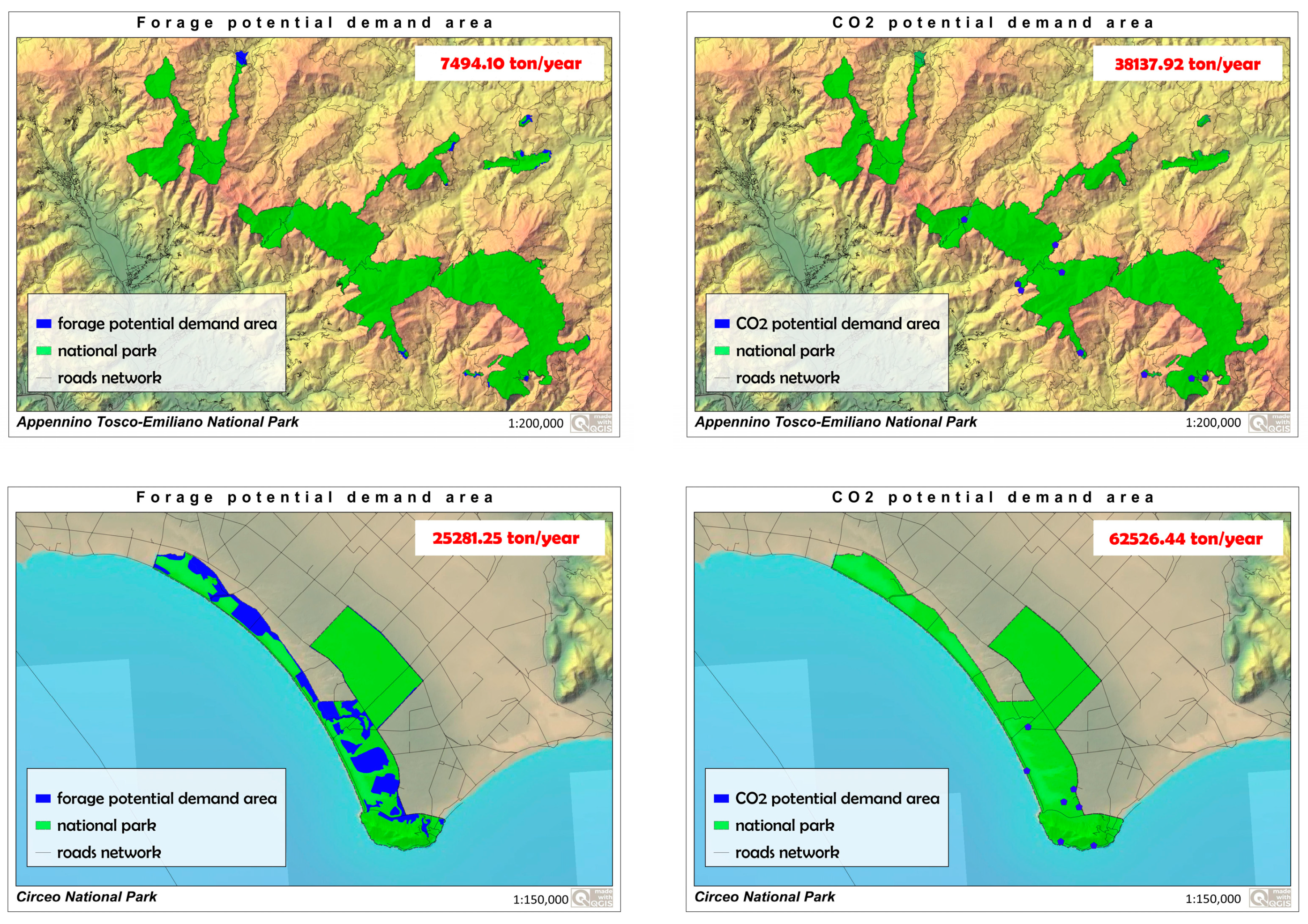
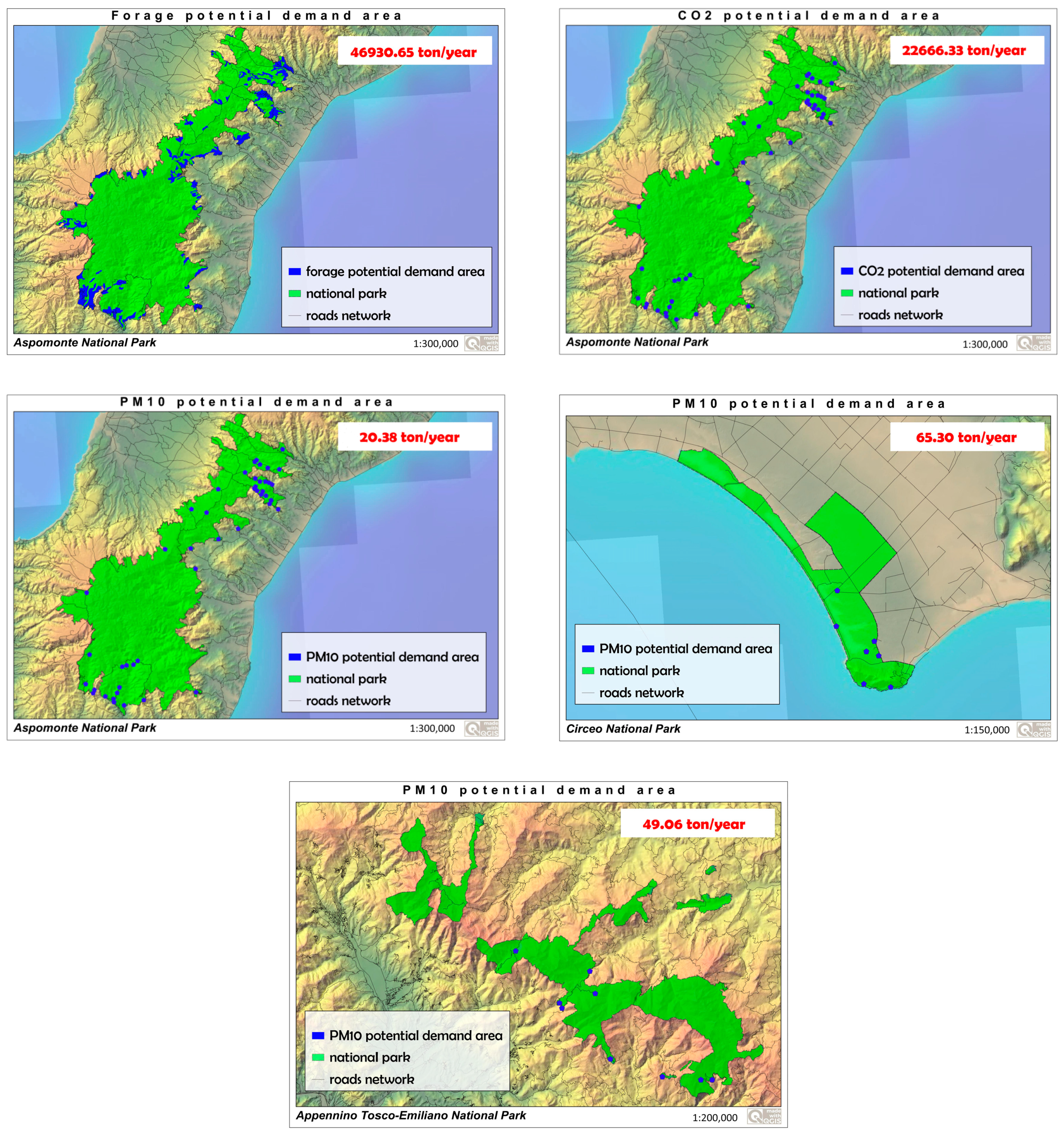
Table 3. Biophysical quantification of supply and demand and economic value by ES. * social cost ** market price.
ESNational ParksDemand
(t/year)
Supply
(t/year)
Economic Value
(€)
Forage
production
Appennino Tosco
Emiliano
7494.1099,409.7612,426,219.56 **
Circeo25,281.255252.92656,615.24 **
Aspromonte46,930.6537,147.664,643,457.03 **
Carbon
sequestration
Appennino Tosco
Emiliano
38,137.92333,280.04124,943,354.20 *
8,042,047.37 **
Circeo62,526.4421,619.98,105,110.55 *
521,689.88 **
Aspromonte22,666.33491,589.16184,291,860.19 *
11,862,046.43 **
Regulation of
local climate (PM10)
Appennino Tosco
Emiliano
49.0652,066.08285,562,143.03 *
Circeo65.3013,518.0074,140,957.98 *
Aspromonte20.38111,770.97613,014,697.90 *
Table 4. The spatial relationship between demand and supply of the investigated ES. Based on Burkhard [31] and Kettunen [88].
ESIndicator FlowIndicator
Demand
Service Providing Units (SPU)
(Hotspots)
Service Benefiting
Areas (SBA)
Spatial Relation SPU-SBAGovernance Protected Areas Benefits
Forage
production
Average forage productionConsumption of forage on farmsAreas of grassland and pasturesHead of cattleIn situ; DecoupledRegional
Private
Carbon
sequestration
CO2 captured by forest biomassPM10 per employee per economic enterpriseForest coverEmployees per economic enterpriseIn situ -
omnidirectional
Global
Regulation of local
climate (PM10)
PM10 captured by
forest biomass
PM10 per employee per
economic
enterprise
Forest coverEmployees per economic enterpriseIn situ -
omnidirectional
Global
Publisher’s Note: MDPI stays neutral with regard to jurisdictional claims in published maps and institutional affiliations.

