
Long-Term Changes in Four Populations of the Spiny Toad, Bufo spinosus, in Western France; Data from Road Mortalities

Institute for Development, Ecology, Conservation and Cooperation, Via G. Tomasi di Lampedusa 33, 00144 Rome, Italy
Conservation 2022, 2(2), 248-261; https://0-doi-org.brum.beds.ac.uk/10.3390/conservation2020017
Submission received: 9 March 2022
/
Revised: 29 March 2022
/
Accepted: 6 April 2022
/
Published: 12 April 2022
(This article belongs to the Special Issue On the Bridge between Conservation Ecology and Environment Management: Contributions of IDECC from Multiple Geographic Contexts)
Abstract
:Habitat fragmentation is widely recognized as a contributor to the decline of biodiversity, with amphibians one of the key groups impacted. To understand the effects of habitat fragmentation on amphibian populations requires long-term data sets showing population trends. In this paper, road mortalities were employed as proxies to describe long-term numbers of four populations of the spiny toad Bufo spinosus in western France during a 17-year period. Road mortalities were found during all months in all populations but were most frequent during October, November and December, the main migratory period. Large females were found significantly more frequently during these migration months, forming 45% of the total sample, compared with their presence from January to September (34.4%). The long-term trends were evaluated using regression analysis of the logarithmic (loge) transforms of annual counts as dependent variables against year as the independent variables. All coefficients showed no significant departure from the 0 hypothetical coefficients, indicative of population stability. This was supported by jackknife analysis, which showed good agreement of the pseudo-regression coefficients with the true equations. Stepwise regression of potential climate impacts on toad numbers suggested rainfall levels in October adjusted to 2- and 3-year lags were involved in driving population change. Road mortality counts were also made during 2020 and 2021 when human movement restrictions were in place due to the COVID-19 pandemic. To estimate the potential impact on this disturbance in the methodology, the Poisson distribution was used to estimate potential differences between what would have been expected counts and the observed counts. The results indicate that the observed mortalities were significantly lower than expected in all four populations.
1. Introduction
Amphibians are now acknowledged as key bio-indicators of ecosystems [1]. However, numerous studies also indicated that they are now one of the most endangered vertebrate groups [2], with habitat loss, climate change, extensive use of agrochemicals, increased UV-irradiation and emerging diseases among the factors cited as the causes for the decline [3,4]. Their vulnerability is in part due to many species being dependent on both aquatic and terrestrial environments, which along with a relatively permeable integument renders them particularly susceptible to environmental changes. Identifying the causes of the declines is problematical since amphibian populations often fluctuate over several orders of magnitude [5,6]. Nevertheless, separating long-term declines from short-term fluctuations is a well-known problem [7,8,9,10] and to understand and verify what factors are involved requires a data base of long-term trends, which may require investment in funding as well as time over many years. Additionally, amphibian populations are often in disequilibrium [11], which may mask long-term trends, but for conservation management programs, they are very much needed [12].
A series of methodologies have been used to estimate long or short-term trends [13]. Included are road mortalities, that as well as being employed as proxies for monitoring population changes [13,14,15,16] were also used to estimate changes in, for example, numbers of mammals [17,18,19,20], lizards [21] and snakes [22,23]. The value of the method when applied to amphibians is illustrated in the study of the common European toad Bufo bufo that showed a strong correlation between road mortalities and numbers arriving at breeding ponds [13]. Road mortalities also facilitate detection of amphibians on the open spaces of road surfaces [2,23] and represent independent replicates if carcasses are removed after counting. This avoids double counting and autocorrelation and when applying regression analysis to long time series the equations have ‘no memory’—counts for one year do not impact on the following year’s counts in a significant way [24].
The spiny toad Bufo spinosus (formerly Bufo bufo in western Europe) is a widespread species of anuran in Europe occupying a range of different habitats, including fragmented landscapes (Figure 1). Mostly active nocturnally [25], they are explosive breeders and are known for breeding-site fidelity [23,26,27,28,29,30]. In the study locality, they migrate to large bodies of water in the later months of the year but reproduce in the early months of the following year. In fragmented habitats they are often constrained to crossroads, usually during the hours of darkness that often results in mortalities. Despite reports of population declines in various regions of Europe [13,31,32], it is listed as “least concern” by the IUCN, but as a common species, it has potential to provide insight into long-term population trends and the health of ecosystems [10]. Numerous studies indicated regional differences in population ecology in both B. spinosus and the related B. bufo (e.g., [5,29,33,34,35,36,37]. A review of long-term changes in amphibian numbers indicated B. spinosus populations were declining at a slightly greater rate than they were increasing (52 % (n = 394) versus 47.5% (n = 360) with n = 4 (0.04%), with populations in the survey showing no change [10]. This suggests a need for additional population data, particularly at the meta-population level and over wider areas of Bufo distribution.
In this paper, a continuous 17-year data set derived from four populations in a region of western France is described. However, unforeseen perturbations in the methodology during 2020 and 2021 due to the COVID-19 pandemic and subsequent changes in road traffic levels necessitated that these data be omitted from the long-term analysis, giving a continuous 15-year data set. The following five questions are addressed:
- (1)
- What are the general long-term population trends in the study area?
- (2)
- Are there differences in long-term numbers between populations?—here defined as subpopulations migrating to different breeding ponds.
- (3)
- To what extent do the populations fluctuate on an annual basis?
- (4)
- (5)
- What impact did the restrictions on human movement due to the COVID-19 pandemic have on road mortalities during 2020 and 2021?
2. Methods
2.1. Study Area
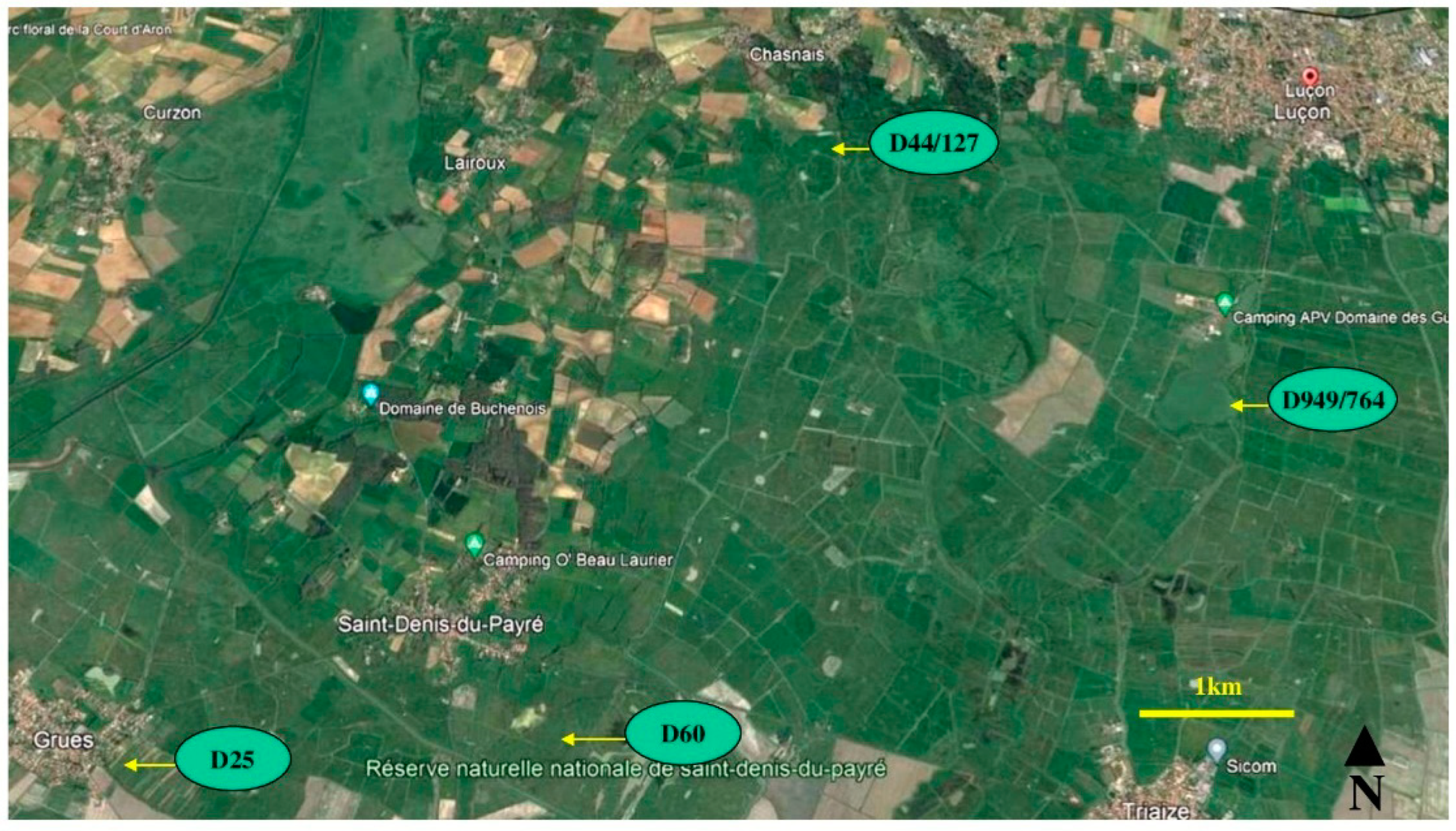
The study area (46°27′ N; 1°53′ W) is a fragmented landscape in Vendee, western France (Figure 2). The locality is dominated by agriculture that had experienced little or no major changes in land use during the study period from 2005 to 2021. The general climate is mild oceanic with mean annual air temperature 13–14 °C. July–August are the hottest and driest months (mean ≈ 22°C) with high precipitation from October until February. Mortalities for B. spinosis were collected on roads (distance ≈ 26 km) between wetland areas south and east of the town of Lucon (D949/D746) and near the villages of Chasnais (D44/D127), Lairoux (D60) and St Denis du Payre and Grue (D25). The straight-line distance between the main breeding ponds are: D949/D746 to D44/D127, 3.7 km; D44/D127 to D60, 3.2 km; D60 to D25, 3.32 km. Figure 3 shows examples of breeding ponds in the study area. The four populations were treated as distinct populations, in part due to the distance between the breeding ponds and known migratory distances or interactions between subpopulations of B. spinosis, which is a function of the distance between them [26,27,30]. For example, interactions between B. spinosus subpopulations were significantly reduced when the distance was greater than 300 m, with none recorded at 830 m [30]. In Germany, it was observed that certain individuals moved more than 1 km [29], but these distances are lower than the distances between ponds in the present study.
2.2. Protocol
Surveying for road B. spinosus mortalities commenced in 2005 on the road networks close to these ponds and were made between four and six times per month from 1 January through to 31 December each year by a single observer on a bicycle at a speed of around 5–10 km/h. Tests of comparison of carcass detection showed that detection increased when using a bicycle compared with motorcar or motorcycle. When found, each individual was measured for snout to vent length (SVL) and removed from the road to avoid double counting. Road traffic volume increased slightly during the study period of 2005 to 2019, with counts showing means of 11.1–60.2 vehicles per hour depending on the road and were greatest on D949 day or night [15].
2.3. Statistical Analysis
Long-term population changes were evaluated using regression analysis with annual counts treated as the dependent variables after transformation to logarithms (Loge) and years as the independent variable. This gives,
where logeN represents road mortalities, x the year (2005 to 2019), m the regression coefficient and b the y-intercept with ε white noise error, which incorporates measurement error and random variation [24]. Due to a zero count for D25 in 2008, the dependent variable was treated as loge(N + 1). The null hypothesis is that logeN (or loge(N + 1)) is stable when m = 0; significant departures from m indicate population change with positive or negative regression coefficients representing population increase or decrease, respectively. Departures from the 0 regression coefficients were evaluated using t-tests at n-2 d.f. Tests for normality of the loge transformed annual counts were made using Anderson–Darling a2 tests. This gave results from a2 = 0.18 to 0.39 and P values from 0.33 to 0.89; hence, all data were normalised before analysis. The Pearson product moment correlation coefficient was used to compare for similarities in monthly counts.
logeN = b + m × x ± ε
Jackknifing was used to estimate the potential errors in the true regression coefficients [24]. This nonrandom method produces repeatable results by systematically removing one-year data sets from the sample and re-applying regression analysis. This gives a series of pseudo-m values and enables comparison of the pseudocoefficients with the true coefficients.
Tests for homogeneity of SVL variance between metapopulations were conducted by Leven’s test for multiple variances. This test is less sensitive to departures from normality and considers the distances of the observations from their sample medians. The null hypothesis is that SVL variance is in agreement between populations, Ho: δ21 … = … δ2k. ANOVA was then used to test for differences in mean SVLs between populations, with the null hypothesis the means are homogenous. Post hoc tests were conducted with Tukey HSD. Leven’s test was also used to test for monthly presence with a null hypothesis of equality of months. Long-term interpopulation correlation of trends between species were assessed with the Pearson correlation coefficient at α = 0.05. To compare the presence of large (≥80 mm SVL) mortalities during the main migration months of October, November and December with their frequencies during January to September, a two-tail z-proportion test was applied at α = 0.05.
To evaluate potential climatic effects on changes in annual counts, stepwise regression using climate data as independent or predictor variables were then compared with annual counts of B. spinosus as the dependent variable. Climatic variables were long-term monthly and total annual rainfall along with annual temperatures during the study period. These data were further analyzed by lagging the climate data to 1, 2 and 3 years previous to annual counts. Initial analysis was by taking the response variable and applying regression analysis to each independent variable for inclusion in the final model [24], with the significance level for independent variable inclusion in the final models α = 0.15. Variables that increased significance of the model were included, those that reduced the significance level were omitted. The regression model has the form
where m1, m2 and m3 … are regression coefficients and x1, x2 and x3 … the variables that had a significant influence on changes in Nbufo. Independent variable selection is arbitrary, but the method is practical when the number of candidate variables is not large [24].
Nbufo = b + m1x1 + m2x2 + m3x3 ……
Climatic information has been sourced from the nearest weather station at La Rochelle-Le Bout Blanc, which is approximately 35 km from the study locality (https://www.infoclimat.fr/climatologie/annee/2000/la-rochelle-le-bout-blanc/valeurs/07315.html (accessed on 4 July 2021)).
Data collected during 2020 and 2021 were not used in the long-term data analysis due to the COVID-19 restrictions on people’s movement and road traffic volumes on B. spinosus road mortalities. The Poisson distribution was used to evaluate any impact this had on road mortalities. The Poisson equation has the form
where the random variable x was defined as the observed number of mortalities during 2020 and 2021, λ the rate parameters as the means of the annual counts from the 15-year time series and e the base natural logarithm. If P (x ≥ λ), this would indicate the observed values of x are reasonable counts and were little influenced by the restrictions. The alternative, P (x < λ), is that the 2020 and 2021 counts are likely due to changes in traffic density and, hence, if included in the analysis would have distorted the long-term trends.
P (x = λ) = λx × e−λ/x!
Data analysis was carried out mainly on Minitab 17 along with VassarStats and various other Internet sites.
3. Results
3.1. Total and Regional Counts
A total of 1180 B. spinosus were recorded on roads between 2005 and 2019. The four subsets were: D949/D764 n = 185 (+2), D44/D127 n = 338 (+9), D60 n = 373 (+13) and D25 n = 333 (+26). The numbers in parenthesis are regional data from 2020 and 2021 and totalled 50 toads. This gives a 17-year total of 1279 toads.
3.2. Monthly Counts
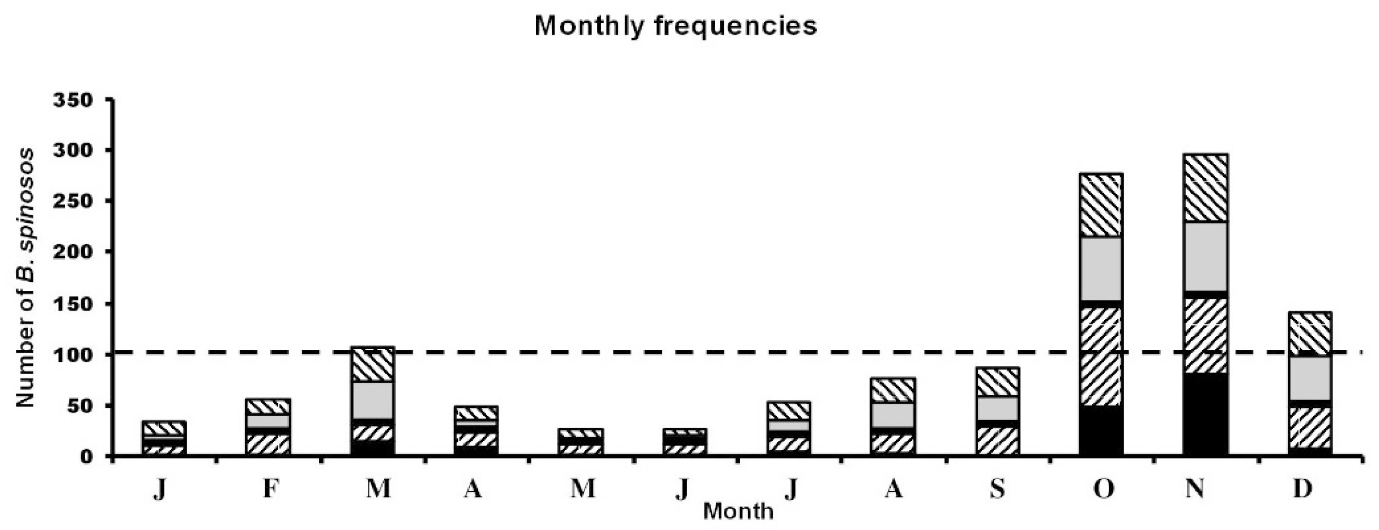
The results here were taken from the 17-year series—that is including 2020 and 2021. Mortalities were found during all months but were negatively skewed towards the latter months in all areas (October, November, December; see Figure 4). A χ2 goodness-of-fit test with a null hypothesis of equality of month presence (expected = 102.1 toads) versus observed monthly numbers indicated a significant departure from the null model, χ2 = 922.6 and P < 0.0001. The Pearson correlation coefficient showed strong monthly correlations between populations, r-values from 0.84 to 0.99 and p-values from 0.001 to 0.0001.
3.3. Frequency of Large Females
In general (all regions pooled), large (≥80 mm SVL) individuals were found more frequently during the main migration months, which were October, November and December, representing 45% of the total sample, compared with the remaining months from January to September, when they reduced to 34.4%. The difference between months was significant z = 3.72 and P = 0.0001.
3.4. Annual Differences in SVL between Populations
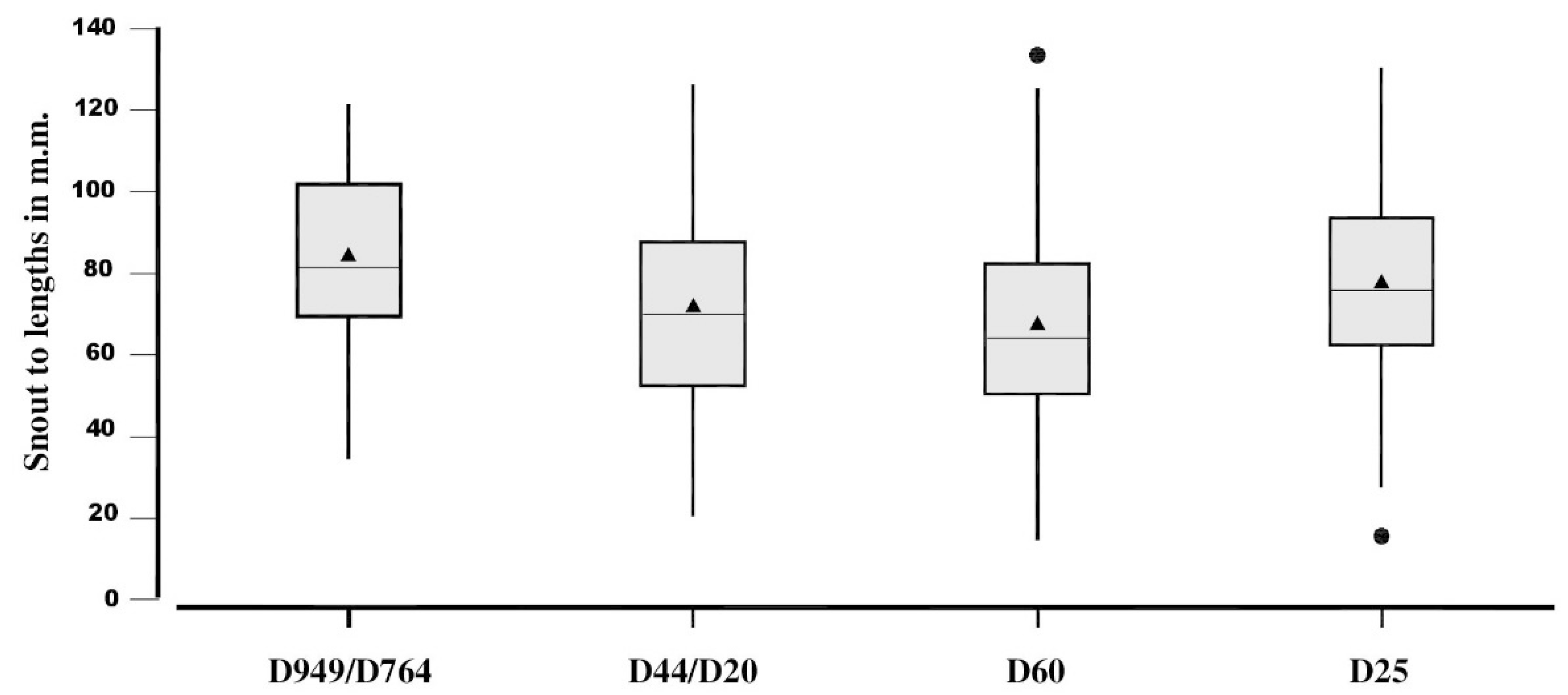
Tests for multiple variances and post hoc Tukey HSD indicated SVL variances in the four populations were in agreement (F = 2.13, P = 0.09). However, ANOVA detected differences between means (F = 27.19, P < 0.0001) with Tukey HSD showing all means differed from each other, with the D949/764 showing the largest individuals (Figure 5; Table 1).
3.5. Long-Term Annual Counts
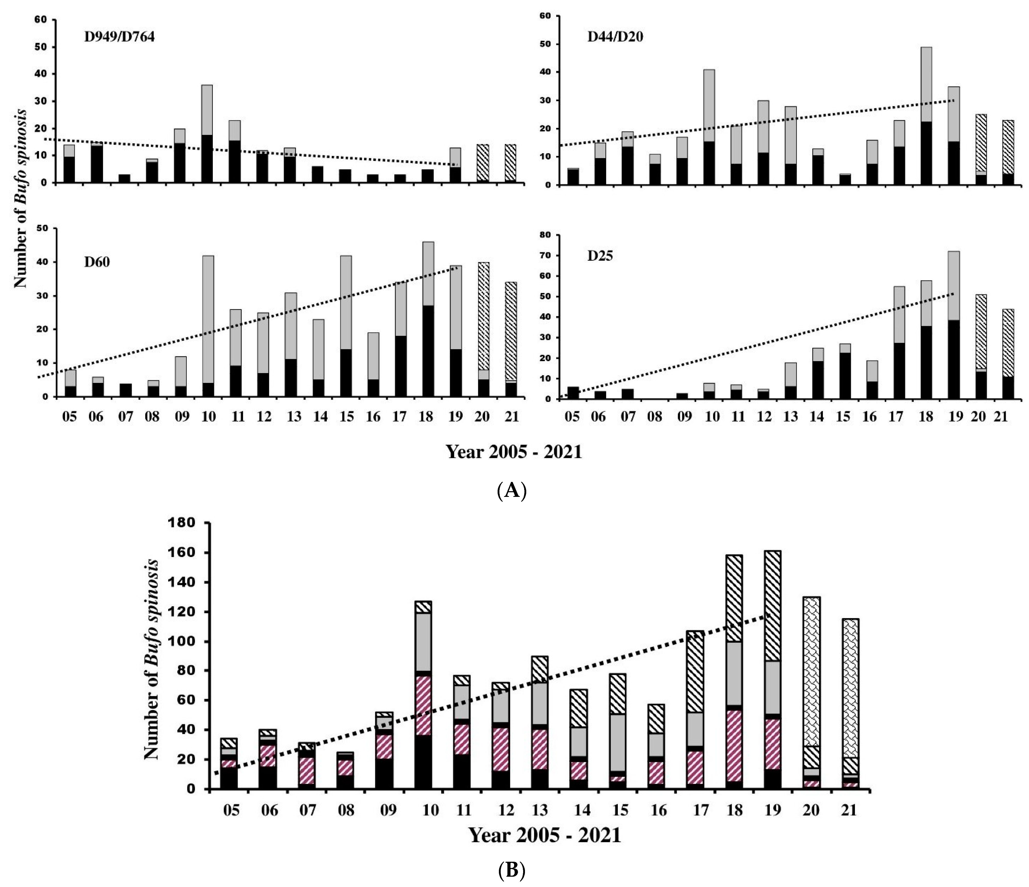
Regression analysis gave positive values of m in three of the four areas, indicating long-term population stability. The population living around D949/D746 showed a negative value of m, but the t-test against the 0 coefficient indicated no significant departure from long-term stability. Regression analysis of pooled data indicated in general populations were stable during the study period (m = 0.1 ± 0.02, t = 4.79). The Jackknife analysis showed good agreement with the true equations but also identified unusually high or low numbers that were unexpected given trends at the time. The results are shown and explained in full in Table 2 along with regression lines derived from the equations in Figure 6A,B.
The means of long-term annual counts ranged from 12 per year (D949/746), 21.8 (D44/D127), 21.7 (D25) and 24.1 (D60) with F = 1.76, P = 0.16. The post hoc Tukey HSD also showed no differences between inter-population variances in counts with P-values from 0.13 to 0.90 and, hence, long-term population fluctuations were similar.
3.6. Rainfall, Temperature and Annual Counts
Since the distances between metapopulations were relatively small, climate events were unlikely to be different and so data were pooled. The stepwise regression was applied to a total of 20 data sets and indicated rainfall as a potential influencer on population change when data were lagged to two or three years previous to the year counts. Three data sets were within the P ≤ 0.15 threshold for inclusion in the final model. These were rainfall levels in October adjusted to a 3-year lag (r = 0.79 and P = 0.01), October adjusted to a 2-year lag (r = 0.64 and P = 0.13) and adjusted to a three-year lag in December (r = 0.63 and P = 0.13). The model gave significance at F = 3.47 and P = 0.05. If, however, ‘three-year lag in December’ was removed, the probability increased to F = 5.61 and P = 0.02, giving a final best-fit model of
where Nbufo is B. spinosus annual counts. These results suggest that rainfall during October lagged to two and three years previous that from the year of annual counts, which is the beginning of the main migratory movement to breeding sites and may be involved as a key population driver.
Nbufo = 207 − 5.66 × rain Octlag2 − 12.3 × rain Octlag3
3.7. Mortalities during 2020 and 2021
The results of the Poisson tests indicated significant departures of the random variables x from the lambda’s (x ≠ λ) in all populations, P < 0.0001 to P = 0.04. This confirms the notion that movement restrictions during 2020 and 2021 had a significant effect in lowering mortalities. Estimates of B. spinosus mortalities in the absence of lower traffic volumes are based on the method in Gotelli and Ellison (2004) but here using
where the estimate E is derived from λ, the rate parameters in the Poisson equations, P the probability that x > λ, with n as the sample sizes. The values of λ and x and subsequent calculations for each population are fully shown in Table 3.
E = P × λ + n
4. Discussion
4.1. General Considerations
The results presented here give good insight into questions 1 and 2, indicating that generally all four populations showed asynchronous long-term trends. However, when data from the four populations were pooled, the results showed general stability over the wider area (Figure 6B). Counts from the D949/D746 area were the most frequent during the early period from 2005 but declined to the 4th rank by 2013 and remained so to the end of the study period. If the populations are operating as metapopulations, this would suggest that asynchronous dynamics may operate as a buffer against the likelihood of simultaneous population crashes and extinctions [40] due to varying degrees of exchange between breeding populations. Hence, although B. spinosus is well known to be philopatric to breeding ponds, some individuals may travel extensively, often over 1 km [29], and potentially colonise areas with depleted numbers. However, interactions between breeding populations apparently declined with increasing distances between breeding ponds, with no interactions above 800 meters, but many individuals (up to 21% of the population) may visit different breeding ponds [30]. Data from the D25 area, for instance, showed relatively sudden and major increases in numbers beginning in 2013 and by the following year the highest counts of the four areas (Figure 6A). This was mirrored by similar increases in live counts in this area. In contrast, numbers in the D44/D127 and D60 areas were generally stable throughout the study period and, hence, it is conceivable that individual toads from these areas could potentially recolonize the D949/D764 area due to the distances between pond breeding areas (Figure 1), albeit in low numbers given our understanding of toad movements.
What drove the relatively sudden increases around the D25 area? The construction of several new ponds in the locality area during the study period may be important. For example, created ponds have been shown to provide partial mitigation for the loss of the natural breeding areas for amphibians [40,41,42,43]. Game fish species are present in the larger ponds (Figure 2) and ornamental fish are often introduced into many larger garden ponds (including one next to D127), which is a known associated factor in toad breeding pond preference [2]. For B. spinosus, predatory fish may positively impact on the numbers of alien crayfish Procambarus clarkia that are well-known predators on all stages of amphibian development including adults [44], thus enhancing larvae survivorship. Only one potential breeding pond was established in the other areas during the study period and that was adjacent to the D127, but this was very close to an already major B. spinosus breeding pond with game fish present (Figure 2), while the new pond did not have any game fish. This new pond was quickly colonized by P. clarkia, which in subsequent years impacted the numbers of early amphibian colonizers, with only Rana dalmatina continuing to use it as a breeding site, albeit in low numbers thereafter [16]. Created ponds have also been shown to provide partial mitigation for the loss of the natural amphibian breeding habitat due to differences in hydrologic regimes, vegetation and surrounding terrestrial habitats between created ponds and natural wetlands [42].
Theory predicts, and is supported by studies, that the survival of adults in a population is crucial for the capacity of a population for growth and long-term stability [43,44]. A positive finding of the present study was the long-term presence, as proportions of total annual numbers, of large females in all four samples. Some of these individuals were particularly large (110 mm + SVL) suggesting good age spans and, hence, high reproductive potential. Female common toads (Bufo bufo) in the UK were found to reach life spans of 9 years with males attaining 6 years [43], although in harsh environments females may take 3 to 7 years to reach maturity and many reproduce only once in a lifetime [36)]
The finding that in all four populations annual counts fluctuated extensively (question 3) is a natural dynamic in amphibians [7,45], as are local extinctions, the latter event observed in the green frog Pelophylax lessonae in the study locality [6]. Such dynamics are often associated with pond living/breeding biphasic species, where population fluctuation is often determined by changes in the environment [10] with populations likely to be declining most of the time, followed by short periods of increases in numbers [10]. A classic example is a study of B. americanus that initially showed an 18-year trend of long-term population decline but with a rapid recovery during the following 7-year period [46,47]. The data from the present study, albeit with shorter time periods, along with other studies, support these trends [6,14]. Population stability has been shown not to be a key requirement for long-term amphibian persistence, since many species that show high fluctuations also have a high capacity for recovery [10], even from local extinctions [2,6,14].
4.2. Comparisons with Sympatric Amphibians
Long-term trends were, in general, in good agreement with population trends in sympatric amphibians recorded in previous studies [6,16]. For example, high numbers of B. spinosus around 2009–2012 were similarly observed in sympatric Triturus marmoratus, Hyla arborea and Pelophylax lessonae [6], with Rana dalmatina also showing comparable long-term trends, albeit based on combined long-term spawn mass and road mortality counts [16]. The high counts recorded during 2009–2012 were followed by a decline, then numbers increased again from approximately 2016. Interspecific similarities were also found in the stepwise regression for climatic data, where lagged rainfall patterns during periods of high movement in November and December were highlighted as potential population influencers [6].
4.3. Rainfall and Temperature
The finding of rainfall (albeit lagged rainfall data—question 4) as a potential driver has been shown to affect breeding populations of other species of amphibians by influencing breeding activity and past recruitment [10,11]. Rainfall can alter amphibian habitats, especially water levels, for example small ponds and ditches can dry out early before metamorphosis is complete, while in some years flooding can move spawn to unsuitable habitats (unpublished data for R. dalmatina). Rainfall can also alter water temperatures that in turn may influence sex ratios [38]. The effects of such events on B. spinosus in the study locality are probably much fewer compared with sympatric amphibians given the large water bodies they use for breeding. However, when B. spinosus data were pooled, long-term numbers showed remarkable stability and indeed numbers increased compared with five sympatric species [6,16].
4.4. Impact of Lockdown Restrictions
In the present study, lockdowns also impacted sampling frequency, although toad carcasses often have very long duration time on roads [15] and, hence, it is proposed that the observed numbers of carcasses were indeed reduced and not simply an artefact of sampling during lockdown. Therefore, the results from the Poisson distribution from data gathered during the pandemic give an unexpected insight on the significant impact of traffic on toad mortalities during normal times. Previously, researchers have had to rely predominantly on mostly observational approaches to understand road traffic effects on mortalities, but now data from previous years and future years after the anthropause should enable greater understanding of traffic volumes on road mortalities. The data from 2020 and 2021 and the Poisson analysis thus provide an answer to question 5, indicating even short periods of traffic reduction or road closures could be used as part of a management strategy for the conservation of amphibian populations. These may only involve minor changes but could potentially have major benefits for ecosystems and in the longer term, humans [48,49].
4.5. Concluding Remarks
Long-term amphibian time series give insight into the range of natural fluctuations that populations experience and present testable hypotheses of long-term trends, including declines. Monthly time series provide additional information on the expected numbers that enter roads outside the main migratory period of these populations, which is important because in other areas of Europe the main migratory period is during early spring, for e.g., [13,34]. This information, together with long-term data series, is key for implementing mitigation measures to at least reduce road mortalities. However, simple times series are unlikely to provide a detailed understanding of the underlying factors involved in amphibian population trends, especially those with complex life cycles. For example, density-dependent regulation is a possible candidate for long-term regulation, but this may occur at the larval, juvenile or adult stage or even all three stages with the larvae interacting in different ways to the terrestrial stages. This can result in highly complex dynamics and wide fluctuations in adult numbers over long time periods. The crucial role amphibians play in many ecosystems can influence the populations of other species, including snakes [48], emphasising the importance of increasing understanding of changes in their population status, especially the nature of their declines. Future data of long-term time series are a critical first step for understanding amphibian population ecology, but measures to reduce road mortalities have already been in place in several European states, for example, in France where underground tunnels for safe road crossings were installed under the A83 autoroute [50] and in the UK where the British Herpetological Society designed and constructed gully pot ladders to enable amphibians to easily escape from being trapped in roadside drains. These are available at very low price and tests have shown that the ladders have the potential to reduce mortalities significantly and have been used by local authorities, road construction companies and developers [51]. However, simple signposts can also be of value, reminding drivers that they are approaching toad and other amphibians’ road-crossing areas, which is especially useful when the main migratory periods are known.
Funding
This research received no external funding.
Institutional Review Board Statement
The study did not require ethical approval since the data was generated from road mortalities of B. spinosus.
Informed Consent Statement
Not applicable.
Data Availability Statement
The data presented in this study are reported in the tables and figures and not publicly available due to ongoing longitudinal analysis.
Conflicts of Interest
The author declares no conflict of interest.
References
- Colwell, R.K.; Dunn, R.R.; Harris, N.C. Coextinction and persistence of dependent species in a changing world. Annu. Rev. Ecol. Evol. Syst. 2012, 43, 183–203. [Google Scholar] [CrossRef] [Green Version]
- Beebee, T.J.C.; Griffiths, R.A. The amphibian decline crisis: A watershed for conservation biology? Biol. Conserv. 2005, 125, 271–285. [Google Scholar] [CrossRef]
- Wake, D.B. Declining amphibian populations. Science 1991, 253, 860. [Google Scholar] [CrossRef] [PubMed]
- Stuart, S.N.; Chanson, J.S.; Cox, N.A.; Young, B.E.; Rodrigues, A.S.L.; Fischmann, D.L.; Waller, R.W. Status and trends of amphibian declines and extinctions worldwide. Science 2004, 306, 1783–1786. [Google Scholar] [CrossRef] [PubMed] [Green Version]
- Kyek, M.; Kaufmann, P.H.; Lindner, R. Differing long term trends for two common amphibian species (Bufo bufo and Rana temporaria) in alpine landscapes of Salzburg, Austria. PLoS ONE 2017, 12, e0187148. [Google Scholar] [CrossRef] [Green Version]
- Meek, R. Population trends of four species of amphibians in western France; results from a 15 year time series derived from road mortality counts. Acta Oecologica 2021, 110, 103713. [Google Scholar] [CrossRef]
- Pechmann, J.H.K.; Scott, D.E.; Semlitsch, R.D.; Caldwell, J.P.; Vitt, L.J.; Gibbons, J.W. Declining amphibian populations: The problem of separating human impacts from natural fluctuations. Science 1991, 253, 892–895. [Google Scholar] [CrossRef] [Green Version]
- Alford, R.A.; Richards, S.J. Global amphibian declines: A problem in applied ecology. Ann. Rev. Ecol. System. 1999, 30, 133–165. [Google Scholar] [CrossRef] [Green Version]
- Houlahan, J.E.; Findlay, C.S.; Schmidt, B.R.; Meyer, A.H.; Kuzmin, S.L. Quantitative evidence for global amphibian population declines. Nature 2000, 404, 752–755. [Google Scholar] [CrossRef]
- Green, D.M. The ecology of extinction: Population fluctuation and decline in amphibians. Biol. Conserv. 2003, 111, 331–343. [Google Scholar] [CrossRef]
- Green, D.M. Perspectives on amphibian declines: Defining the problem and searching for answers. In Amphibians in Decline: Canadian Studies of a Global Problem; Green, D.M., Ed.; Society for the Study of Amphibians and Reptiles, 1997; pp. 291–308. Available online: https://www.researchgate.net/publication/247167604_Perspectives_on_amphibian_population_declines_defining_the_problem_and_searching_for_answers (accessed on 4 July 2021).
- Scherer, R.D.; Tracey, J.A. A power analysis for the use of counts of egg masses to monitor wood frog (Lithobates sylvaticus) populations. Herpetol. Conserv. Biol. 2011, 6, 81–90. [Google Scholar]
- Cooke, A.S.; Sparks, T.H. Population declines of common toads (Bufo bufo): The contribution of road traffic and monitoring value of casualty counts. Herpetol. Soc. Bull. 2004, 88, 13–26. [Google Scholar]
- Meyer, A.H.; Schmidt, B.R.; Grossenbacher, K. Analysis of three amphibian populations with quarter century long time series. Proc. R. Soc. 1998, 265, 523–528. [Google Scholar] [CrossRef]
- Meek, R. Patterns of amphibian road-kills in the Vendée region of Western France. Herpetol. J. 2012, 22, 51–58. [Google Scholar]
- Meek, R. Temporal trends in agile frog Rana dalmatina numbers: Results from a long term study in western France. Herpetol. J. 2018, 28, 117–122. [Google Scholar]
- Mallick, S.A.; Hocking, G.J.; Driessen, M.M. Road kills of the eastern barred bandicoot (Perameles gunnii) in Tasmania: An index of abundance. Wildl. Res. 1998, 2, 139–145. [Google Scholar] [CrossRef]
- Baker, P.; Harris, S.; Robertson, C.; Saunders, G.; White, P. Is it possible to monitor mammal population changes from counts of road traffic casualties? An analysis using Bristol’s red foxes Vulpes vulpes as an example. Mamm. Rev. 2004, 34, 115–130. [Google Scholar] [CrossRef]
- Widenmaier, K.; Fahrig, L. Inferring white-tailed deer (Odocoileus virginianus) population dynamics from wildlife collisions in the City of Ottawa. In Proceedings of the 2005 International Conference on Ecology and Transportation, San Diego, CA, USA, 29 August–2 September 2005; Irwin, C.L., Garrett, P., McDermott, K.P., Eds.; Center for Transportation and the Environment: San Diego, CA, USA, 2006; pp. 589–602. [Google Scholar]
- Battisti, C.; Amori, G.; De Felici, S.; Luiselli, L.; Zapparoli, M. Mammal roadkilling from a Mediterranean area in central Italy: Evidence from an atlas dataset. Rend. Lincei 2012, 2, 217–223. [Google Scholar] [CrossRef]
- Meek, R. Temporal trends in Podarcis muralis and Lacerta bilineata populations in a fragmented landscape in Western France: Results from a 14 year time series. Herpetol. J. 2020, 30, 19–25. [Google Scholar] [CrossRef] [Green Version]
- Rugiero, L.; Capula, M.; Capizzi, D.; Amori, G.; Milana, G.; Lai, M.; Luiselli, L. Long-term observations on the number of roadkilled Zamenis longissimus (Laurenti, 1768) in a hilly area of central Italy. Herpetozoa 2018, 30, 212–217. [Google Scholar]
- Beckmann, C.; Shine, R. Do the numbers and locations of road-killed anuran carcasses accurately reflect impacts of vehicular traffic? J. Wildl. Manag. 2014, 79, 92–101. [Google Scholar] [CrossRef]
- Gotelli, N.J.; Ellison, A.M. A Primer of Ecological Statistics; Sinauer Associates: Sunderland, MA, USA, 2004; p. 510. [Google Scholar]
- Meek, R.; Jolley, E. Body temperatures of the common toad, Bufo bufo, in the Vendee, France. Herpetol. Bull. 2006, 95, 21–24. [Google Scholar]
- Heusser, H. Uber die Beziehungen der Erdkröte (Bufo bufo L.) zu ihrem Laichplatz. II. Behaviour 1960, 16, 93–109. [Google Scholar] [CrossRef]
- Heusser, H. Die Lebensweise der Erdkrote, Bufo bufo (L.); Das Orientierungsproblem. Rev. Suisse Zool. 1969, 76, 443–518. [Google Scholar] [PubMed]
- Haapanen, A. Site tenacity of the common toad, Bufo bufo (L). Ann. Zool. Fenn. 1974, 11, 251–252. [Google Scholar]
- Sinsch, U. Seasonal changes in migratory behaviour of the toad Bufo bufo; direction and magnitude of movements. Oecologia 1998, 76, 390–398. [Google Scholar] [CrossRef] [PubMed]
- Reading, C.J.; Loman, J.; Madsen, T. Breeding pond fidelity in the common toad Bufo bufo. J. Zool. 1991, 225, 201–211. [Google Scholar] [CrossRef]
- Zuiderwijk, A.; Janssen, I. Results of 14 Years Reptile Monitoring in the Netherlands. In Proceedings of the 6th World Congress of Herpetology, Manaus, Brazil, 18 August 2008. [Google Scholar]
- Cruickshank, S.S.; Ozgul, A.; Zumbach, S.; Schmidt, B.R. Quantifying population declines based on presence only records for Red List assessments. Conserv. Biol. 2016, 30, 1112–1121. [Google Scholar] [CrossRef]
- Gittins, S.P.; Parker, A.G.; Slater, F.M. Population characteristics of the common toad (Bufo bufo) visiting a breeding site in mid -Wales. J. Anim. Ecol. 1980, 49, 161–173. [Google Scholar] [CrossRef]
- Gittins, S.P. The breeding migration of the common toad (Bufo bufo) to a pond in Mid-Wales. J. Zool. Lond. 1983, 199, 555–562. [Google Scholar] [CrossRef]
- Griffiths, R.A.; Harrison, J.D.; Gittins, S.P. The breeding migrations of amphibians at Llysdinam pond, Wales: 1981–1985. In Studies in Herpetology; Rocek, Z., Ed.; Charles University: Prague, Czech Republic, 1986; pp. 543–546. [Google Scholar]
- Kuhn, J. Lebensgeschichte und demographie von erdkrötenweibchen Bufo bufo (L.). Z. Feldherpelopie 1994, 1, 3–87. [Google Scholar]
- Schabetsberger, R.; Langer, H.; Jersabek, M.; Goldschmid, A. On age structure and longevity in two populations of Bufo bufo (LINNAEUS, 1758) at high altitude breeding sites in Austria. Herpetozoa 2000, 13, 187–191. [Google Scholar]
- Wallace, H.; Badawy, G.M.I.; Wallace, B.M.N. Amphibian sex determination and sex reversal. Cell. Mol. Life Sci. 1999, 55, 901–909. [Google Scholar] [CrossRef] [PubMed]
- Matsuba, C.; Miura, I.; Merilä, J. Disentangling genetic vs. environmental causes of sex determination in the common frog, Rana temporaria. BMC Genet. 2008, 9, 3. [Google Scholar] [CrossRef] [PubMed] [Green Version]
- Smith, M.A.; Green, D.M. Dispersal and the metapopulation paradigm in amphibian ecology and conservation: Are all amphibian populations metapopulations? Ecography 2005, 28, 110–128. [Google Scholar] [CrossRef]
- Pechmann, J.H.K.; Estes, R.A.; David, E.; Scott, D.E.; Whitfield Gibbons, J. Amphibian colonization and use of ponds created for trial mitigation of wetland loss. Wetlands 2001, 21, 93–111. [Google Scholar] [CrossRef]
- Petranka, J.W.; Kennedy, C.A.; Murray, S.S. Response of amphibians to restoration of a southern appalachian wetland: A long-term analysis of community dynamics. Wetlands 2003, 3, 1030–1042. [Google Scholar] [CrossRef]
- Gittins, S.P.; Kennedy, R.I.; Williams, R. Aspects of the population age- structure of the common toad (Bufo bufo) at Llandrindod Wells lake, mid-Wales. Br. J. Herpetol. 1985, 6, 447–449. [Google Scholar]
- Ficetola, G.F.; Siesa, M.E.; Manenti, R.; Bottoni, L.; De Bernardi, L. Early assessment of the impact of alien species: Differential consequences of an invasive crayfish on adult and larval amphibians. Divers. Distrib. 2011, 17, 1141–1151. [Google Scholar] [CrossRef]
- Semlitsch, R.D.; Scott, D.E.; Pechmann, J.H.K.; Gibbons, J.W. Structure and dynamics of an amphibian community: Evidence from a 16-year study of a natural pond. In Long-Term Studies of Vertebrate Communities; Cody, M.L., Smallwood, J.A., Eds.; Academic Press: San Diego, CA, USA, 1996; pp. 217–248. [Google Scholar]
- Bragg, A.N. Population fluctuation in the amphibian fauna of Cleveland County, Oklahoma during the past twenty-five years. Southwest. Nat. 1960, 5, 165–169. [Google Scholar] [CrossRef]
- Bragg, A.N. Decline in toad populations in central Oklahoma. Proc. Oklahoma Acad. Sci. 1954, 33, 70. [Google Scholar]
- Zipkin, E.F.; DiRenzo, G.V.; Ray, J.M.; Rossman, S.; Lips, K.R. Tropical snake diversity collapses after widespread amphibian loss. Science 2020, 367, 814–816. [Google Scholar] [CrossRef] [PubMed]
- Manenti, R.; Mori, E.; Di Canio, V.; Mercurio, S.; Picone, M.; Ca, M.; Brambilla, M.; Ficetola, G.F.; Rubolini, D. The good, the bad and the ugly of COVID-19 lockdown effects on wildlife conservation: Insights from the first European locked down country. Biol. Conserv. 2020, 249, 108728. [Google Scholar] [CrossRef] [PubMed]
- Mougey, T. Des tunnels pour batraciens. Cour. Nat. 1996, 155, 22–28. [Google Scholar]
- Mcinroy, C.; Rose, T. Trialling amphibian ladders within roadside gullypots in Angus, Scotland: 2014 impact study. Herpetol. Bull. 2015, 132, 15–19. [Google Scholar]
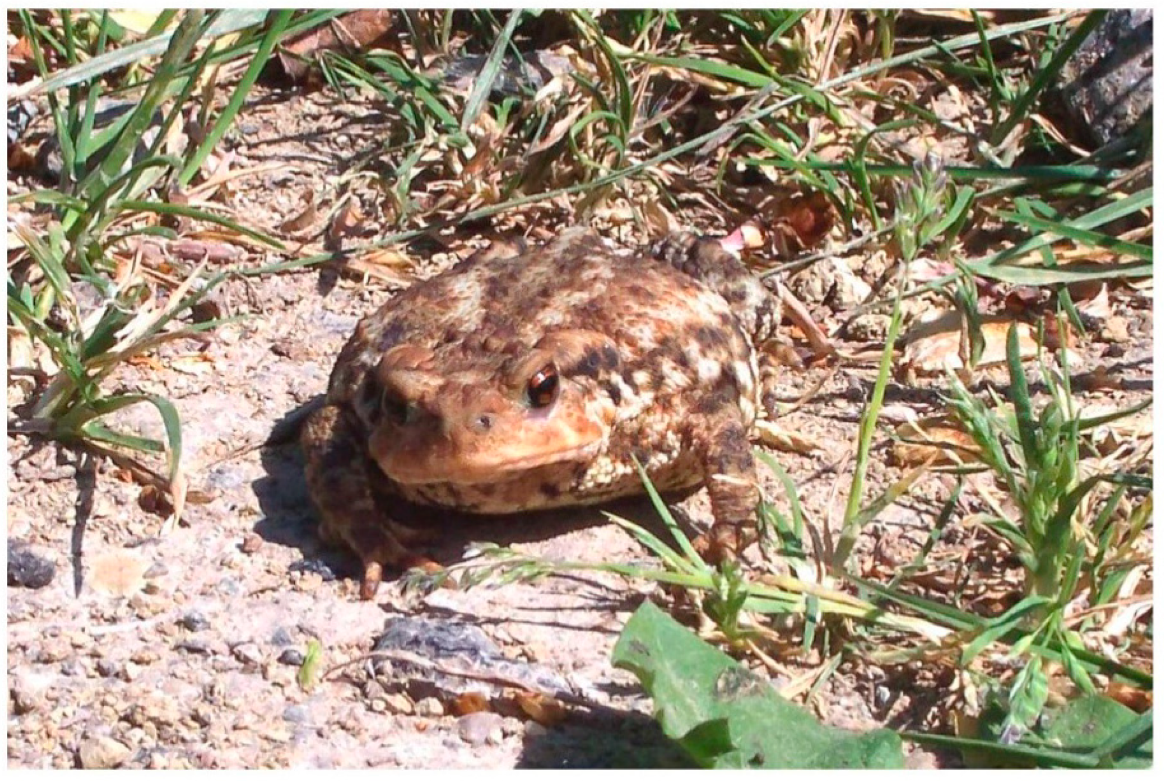
Figure 1.
Example of a B. spinosis (female).

Figure 2.
Map of the general study area with ponds shown in Figure 3 identified.
Figure 2.
Map of the general study area with ponds shown in Figure 3 identified.

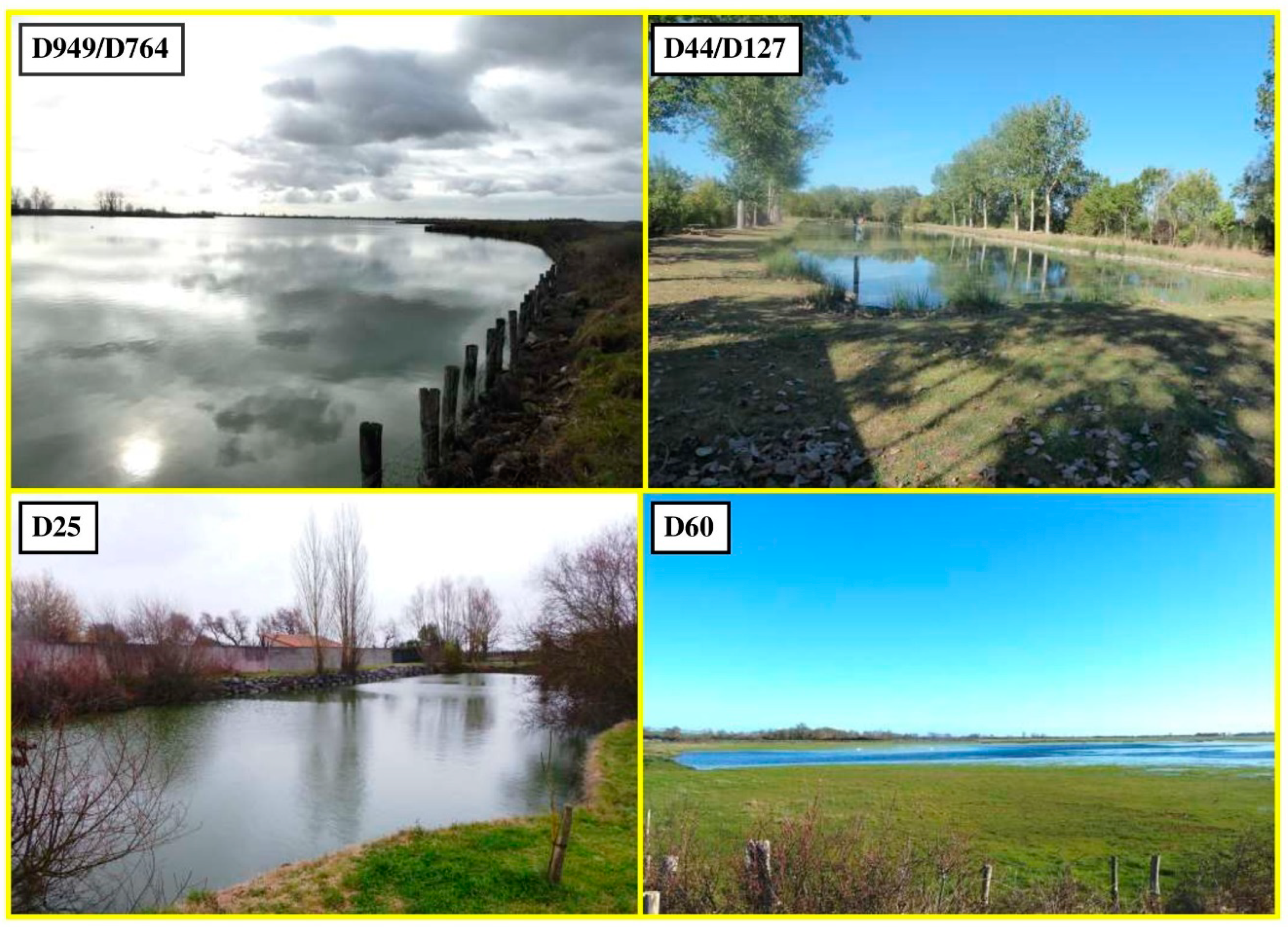
Figure 3.
Examples of toad breeding ponds in the study area labelled with road numbers where mortalities from crossings were found.
Figure 3.
Examples of toad breeding ponds in the study area labelled with road numbers where mortalities from crossings were found.

Figure 4.
Monthly counts for all populations. Black bars indicate D949/ D764 area, grey D60, forward hatched D25 area and backward hatched D44/D127. The broken line indicates expected frequencies under a null hypothesis of equality of monthly counts. See text for other details.
Figure 4.
Monthly counts for all populations. Black bars indicate D949/ D764 area, grey D60, forward hatched D25 area and backward hatched D44/D127. The broken line indicates expected frequencies under a null hypothesis of equality of monthly counts. See text for other details.

Figure 5.
Box plots of SVL distributions of the four populations. Gray boxes indicate central 50% of the samples, the horizontal line and triangle within the box indicate the medians and means, respectively. The bottom of the boxes are situated at the first quartile (Q1) and the top the third quartile (Q3). The vertical lines are the normal ranges and the circles are outliers, unusually large or small values. See text for further details.

Figure 6.
(A) Histograms showing mortality counts from 2005 to 2021 for all four areas. Solid bars represent large females (≥80 mm SVL), gray bars smaller individuals (either sex) and scaled bars represent estimates derived from the Poisson distribution for 2021 and 2022. Note differences of scale between the y-axes. (B) Pooled histograms from all four regions. Black bars represent D949/D764, backward cross-hatched bars D44/D127, gray bars D60 and forward-hatched bars D25. Dotted lines were calculated from the regression equations for each population given in Table 2. See text for further details.


Table 1.
Means and standard deviations and skewness distributions of SVLs in the four populations.
| D949/D746 | D44/D127 | D60 | D25 | |
|---|---|---|---|---|
| Means | 83.7 ± 20.2 | 71.3 ± 73.8 | 66.9 ± 22.2 | 77.3 ± 23.1 |
| Skewness | −0.07 | 0.24 | 0.47 | −0.08 |
| n | 187 | 347 | 386 | 359 |
Table 2.
Regression coefficients (m) relating annual mortalities between 2005 and 2019 along with results of the Jackknife analysis (mJK). For m, the ±values are standard errors of the coefficients and the t-tests against the 0 regression coefficients. When m was positive, numbers were generally increasing; when m was negative, numbers were decreasing. The latter was only found for D949/D764, but the result was not significant. For the Jackknife results, means and standard errors are the mean values of the 15-year pseudoregression coefficients with their standard deviation. Right column identifies years when influence functions were detected, indicating unexpected low (L) or high numbers (H) given current trends at the time. All t-tests were set at n − 2 years (15 − 2 = 13 years). See text for further details.
| Area | m | ±SE | t | P | Mean JK m | Mean JK Std Error | P | Influence Function |
|---|---|---|---|---|---|---|---|---|
| D949/D764 | −0.07 | 0.04 | 1.58 | 0.14 | −0.07 | 0.046 | 0.14 | 2007 (L) |
| D44/D127 | 0.05 | 0.04 | 1.41 | 0.18 | 0.03 | 0.055 | 0.20 | 2015 (L) |
| D60 | 0.15 | 0.03 | 4.84 | <0.0001 | 0.15 | 0.031 | <0.0001 | 2010 (H) |
| D25 | 0.23 | 0.04 | 6.20 | <0.0001 | 0.22 | 0.039 | <0.0001 | 2008 (L) |
Table 3.
Poisson probabilities that road mortality counts during 2020 and 2021 are a true measure of expected mortalities P (λ = x). The rate parameters (λ) are derived from the mean values of the long-term annual counts (15 years) and the random variable x from the observed numbers in each area during 2020 and 2021. The likelihood that the true counts were greater than the rate parameters (x > λ) ranged from 84–100% during 2020 and greater than 99% for 2021.
| 2 | λ Rate Parameter | x Random Variable | P (λ = x) | P (x > λ) |
| D949/764 | 12 | 1 | <1% | >99.9% |
| D44/127 | 15 | 5 | <1% | >99.9% |
| D60 | 24 | 8 | <1% | >99.9% |
| D25 | 22 | 15 | 0.03% | 92.3% |
| 2020 total n | 29 | |||
| λ Rate Parameter | x Random Variable | P (λ = x) | P (x > λ) | |
| D949/764 | 12 | 1 | <1% | >99.9% |
| D44/127 | 15 | 4 | <1% | >99.9% |
| D60 | 24 | 5 | <1% | >99.9% |
| D25 | 22 | 11 | 0.004% | >99.9% |
| 2021 total n | 21 |
Publisher’s Note: MDPI stays neutral with regard to jurisdictional claims in published maps and institutional affiliations. |
© 2022 by the author. Licensee MDPI, Basel, Switzerland. This article is an open access article distributed under the terms and conditions of the Creative Commons Attribution (CC BY) license (https://creativecommons.org/licenses/by/4.0/).
Share and Cite
MDPI and ACS Style
Meek, R. Long-Term Changes in Four Populations of the Spiny Toad, Bufo spinosus, in Western France; Data from Road Mortalities. Conservation 2022, 2, 248-261. https://0-doi-org.brum.beds.ac.uk/10.3390/conservation2020017
AMA Style
Meek R. Long-Term Changes in Four Populations of the Spiny Toad, Bufo spinosus, in Western France; Data from Road Mortalities. Conservation. 2022; 2(2):248-261. https://0-doi-org.brum.beds.ac.uk/10.3390/conservation2020017
Chicago/Turabian StyleMeek, Roger. 2022. "Long-Term Changes in Four Populations of the Spiny Toad, Bufo spinosus, in Western France; Data from Road Mortalities" Conservation 2, no. 2: 248-261. https://0-doi-org.brum.beds.ac.uk/10.3390/conservation2020017