
Numerical Integration of Weight Loss Curves for Kinetic Analysis


Department of Chemical Engineering, University of Alicante, 03690 Alicante, Spain
Thermo 2021, 1(1), 32-44; https://0-doi-org.brum.beds.ac.uk/10.3390/thermo1010003
Submission received: 30 January 2021
/
Revised: 1 March 2021
/
Accepted: 2 March 2021
/
Published: 5 March 2021
Abstract
:Research abounds in the literature on kinetic analyses using thermogravimetric (TG) runs. Many of these studies use approximations of integral or derivative forms of the kinetic law and all of them use programmed temperatures. In the present work, a numerical integration procedure was discussed and applied to different examples. We focused on materials presenting a single decomposition curve as well as other materials with more complex processes. Different examples were explored, and the methodology was applied to a number of wastes such as coffee husks, polystyrene and polyethylene. In all cases, the actual temperature measured by thermocouples close to the sample is used, and several runs are fitted using the same kinetic parameters, giving robustness to the results.
1. Introduction
The literature offers several weight loss curve fitting methods in order to perform kinetic analyses. The most commonly used linear forms of the weight loss equation include the methods of Freeman and Carrol [1], Newkirk [2], Horowitz and Metzger [3], Coats and Redfern [4] and Friedman [5]. All these methods use the n-th order kinetic law and seek to linearize the form of the derived differential equation and uses the data of a single run.
To carry out the kinetic calculations, almost all of these (old) methods apply temperatures programmed using a thermobalance, rather than the actual temperature read by a thermocouple that should ideally be placed very close to the sample. Applying the programmed heating rate (T = T0 + HR·t) instead of the experimental relation T = f(t) can lead to major calculation errors if a strong exothermic or endothermic process is being produced [6]. A simple heating rate programme is not actual temperature, insofar as it is not possible to account for the sample’s temperature variations resulting from the reactions that are taking place. These variations can only be taken into account by performing a step-by-step numerical integration of the necessary differential equations.
Another important drawback of these methods is that they are difficult to apply to materials that decompose over several different processes, i.e., to TG curves presenting more than one process. The existence of more than one process is easily observable in the weight-loss curve derivative, where several relative minima would be found. Nevertheless, all processes would be superposed, and usually, no clear separation would be found, implying that the methods mentioned above are not applicable.
An additional downside of almost all of these methods (except isoconversional methods) is that they use the data obtained for one heating rate only. A number of studies [2,7,8] have shown that the fit of a single curve can be satisfactory using several models, based on a very similar quality of the obtained fit. For example, a single TG polyethylene decomposition curve can be satisfactorily fitted using the Prout-Tompkin model with n = −0.5, m = −1, k0 = 6.1 × 10¹¹ s−1 and E/R = 24,415 K, as well as with Avrami’s model, with n = m = 1.53, k0 = 3.02 × 10¹⁰ s−1 and E/R = 21,273 K [9,10]. In these models, E/R is the activation energy (divided by the constant of the gases), k0 is the pre-exponential factor and the values of ‘m’ and ‘n’ represent reaction and nucleation orders.
In this way, for a given material, a range of kinetic models can be found in the literature [11], and different kinetic constants can be obtained using the same model, applied to experiments conducted under different operating conditions. It is possible that there are small differences between experiments carried out by two different laboratories, but the curves obtained should be very similar, as well as the values of the kinetic constants. It is also common to find several dynamic TG fitted to a kinetic model, where a change in kinetic constants is allowed when varying the HR [12] and/or the conversion [10,11,13], and where, occasionally, changes in the reaction mechanism are allowed at the different HRs.
However, it has been shown on many occasions that the same kinetic model can explain a set of dynamic TG with a set of kinetic constants, without the heating rate having to vary [6,14,15,16,17,18]. A more robust model would be able to explain the results obtained under different conditions based on a set of kinetic parameters, without this variation requirement. Undeniably, we should not contemplate a change of mechanism, unless there is other evidence of this change in the mechanism. The apparent kinetics observed in a decomposition process, as in any other type of process, must be the result of all the different processes included. The process (or processes) that control the reaction may vary under different experimental conditions, and consequently, different mechanisms may appear. Clearly, if such a process is correlated with a simple model, different constants, at least, must be obtained under different conditions. However, if the model is more elaborate, a single set of kinetic constants should allow representing the observed phenomenon. The mechanism’s representative kinetic law must be valid for any set of experiments conducted under dynamic or isothermal conditions, and, ideally, under any temperature programme [6]. Note that the kinetic treatment of TG curves never gives information about the mechanisms of decomposition. The reactions are not directly accessible by the TG experiments and a complementary method is needed to get this information.
In this work, we give a step-by-step explanation of how to perform the numerical integration of differential equations for simple and complex materials, and we discuss valid models for the thermal decomposition of coffee husks, PS (polystyrene) and PE (polyethylene) as examples of materials.
2. Numerical Methods for Simple Materials Based on One Process Only
2.1. Theoretical Background
Regarding the thermal decomposition of a simple material (or waste), a single chemical reaction would represent the decomposition, for example:
where a material ‘F’ decomposes producing a fraction of solids, with a yield coefficient ‘s’ kg solid/kg decomposed, and a fraction of gases, which, when cooled, can produce tars and permanent gases. The weight measured using the thermobalance would be that corresponding to the mass of ‘F’ and the solid ‘S’ formed, because the equipment does not allow distinguishing between the non-decomposed sample and the solid formed. We thus obtain, for the weight fraction measured at any time:
Many kinetic formulations of solid-state reactions have assumed that the homogeneous gas phase kinetic equation can be applied [19,20,21], in such a way that the transformation rate during a reaction is the product of two functions, one depending solely on the temperature, T, and the other depending solely on the transformed fraction. Consequently, for a single reaction, such as that presented in S1, the kinetic expression is, at any time, as follows:
where ‘w’ is the weight fraction or mass fraction of the species being decomposed. The f(w) function depends on the controlling mechanism. The kinetic constant k can be expressed by an Arrhenius law:
Some of the usual forms of f(w), depending on the controlling mechanism, can be found in literature [22,23].
In classical kinetic analysis methods, a f(w) is selected [10]; the differential Equation (2) with the selected f(w) is then linearized, the corresponding plot is drawn up, and the kinetic constants are obtained from the slope and ordinate values.
One of the simplest forms of the function f(w) is the n-th order reaction. In this case, Equation (2) can be written as follows:
Worthy of note, in the previous equation T is a function of time, depending on the temperature programme used in the run T = f(t). In any event, this differential equation is subjected to the initial condition:
w = 1 for t = 0
Using a finite approximation method, a variable increment can be used in Equation (4) and:
The superscript ‘t + t’ and ‘t’ refers to the values of the function at times ‘t + t’ and ‘t’, respectively. In this way:
For a particular run, the thermobalance will give the exact temperature programme followed by the equipment, together with the run’s weight or mass fraction, i.e., t-T-w values. Assuming a kinetic triplet k0, E/R and n value, one can very simply integrate Equation (6) using a particular value of Δt and compare the calculated w-t curve values with that of the experimental one. Usually, the same t value as that of the experimental data is chosen, allowing to directly compare experimental and calculated data, and to use the actual temperature measured at the reaction point T = f(t).
2.2. Application to Some Examples
First, we will use this simple method to simulate different runs for a given kinetic triplet or simulate curves obtained based on different kinetic constants. The spreadsheet used for this calculation is available in the Supplementary Material of the present publication (Spreasheet1: simulations of weight loss curves.odt). Figure 1 shows the simulation of a decomposition curve obtained at one constant heating rate (HR) of 10 K/min for the first order (n = 1) with two different preexponential factor values (k1 = 106 s−1 and k2 = 107 s−1), and two activation energy values (E1/R = 12,500 K and E2/R = 15,000 K). Here, we can appreciate the effect of the change in both parameters. Many authors have found that a compensation effect exists between the preexponential factor and the activation energy, in such a way that different combinations of these parameters produce the same TG curve [24,25]. This is not completely true, as the compensation effect can be broken when considering different TG curves obtained under different experimental conditions and fitted with the same set of kinetic constants [7,14,26].
Figure 2 shows the effect of the reaction order simulation of a decomposition curve obtained at one constant heating rate (HR) of 10 K/min, with the preexponential factor k0 = 106 s−1, E/R = 15,000 K and reaction orders of 1, 2 and 0.5. Generally, low orders produce a sharp curve, whereas high values generate smoother curves.
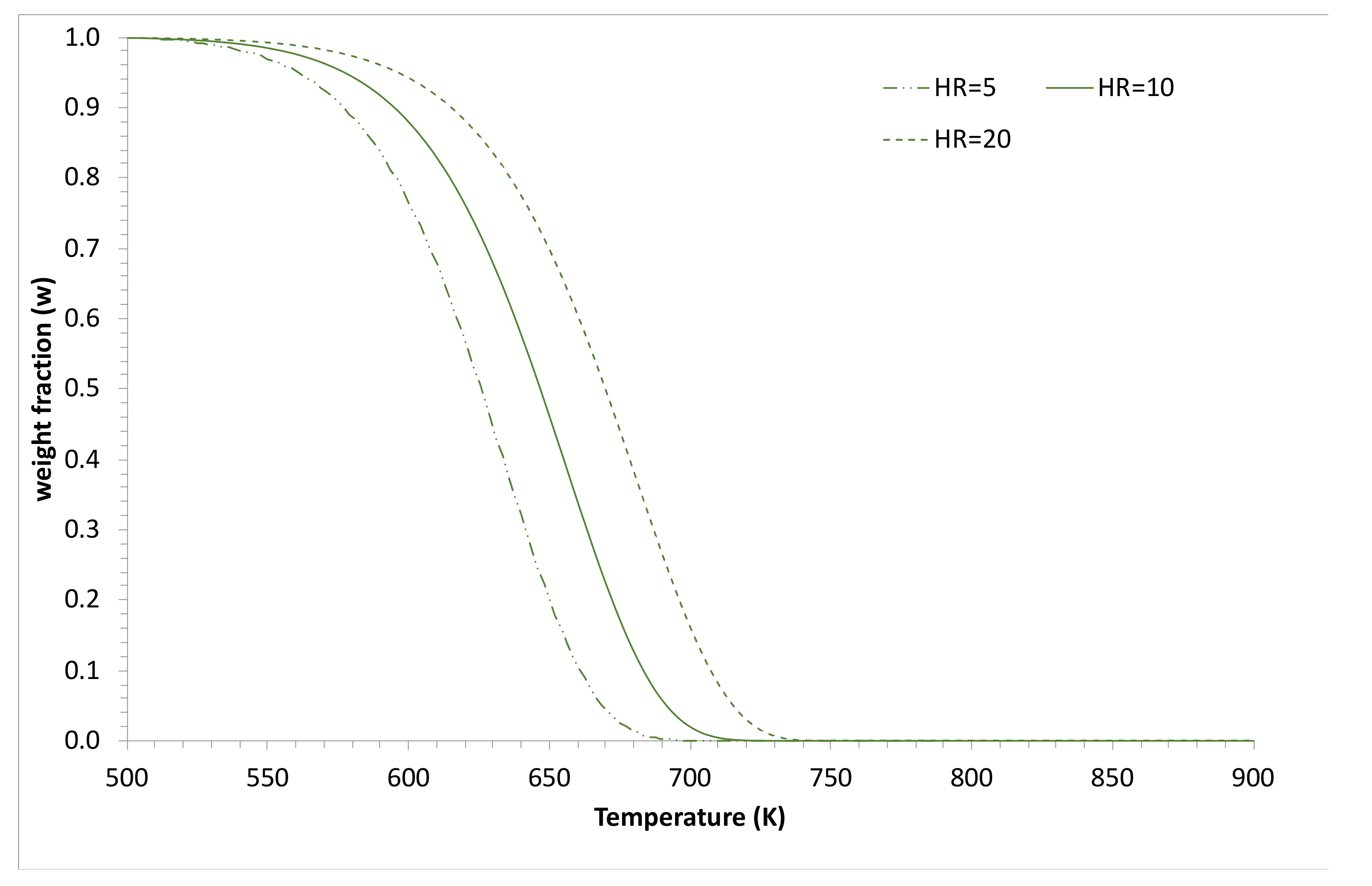
The effect of the heating rate on the curve’s position can also be easily simulated. Figure 3 and Figure 4 show two very different behaviours. On the one hand, Figure 3 (simulation based on k0 = 106 s−1, E/R = 12,500 K, n = 1) shows a case where the curve moves appreciably at higher temperatures when increasing the heating rate, whereas the process in Figure 4 (simulation based on k0 = 1026 s−1, E/R = 48,100 K, n = 1) does not move to the same extent. Worthy of note, no other changes were introduced into the simulation, i.e., a kinetic triplet allows fitting the different behaviours of many materials, without any kinetic parameter modifications, whether in the degree of decomposition or heating rate.
Having explained how the TG curve was calculated for certain parameters, we will now move on to finding the best kinetic values for a given material. For this, we will need an optimisation method [27].
The optimisation of kinetic constants requires defining an objective function. The most common condition for the objective function is to minimise the square differences (although other objective functions can be used) [28,29,30,31]. The most widespread specific objective function (OF) form is:
where wcalj and wexpj are the calculated and experimental values of the weight fraction, and the sub-index ‘j’ refers to a point in an experiment ‘j’. More complex forms taken by the OF can be used and have been discussed elsewhere [26]. To make the calculation more accurate, different runs are usually performed under different experimental conditions (generally a different temperature programme) simultaneously, using the same kinetic model and parameters. In this case, the formal expression of the OF would be:
where the subindex ‘k’ represents different runs.
The fitting of runs performed under different conditions at the same time has been shown to be a valid method to distinguish an actual model [5,32] and to solve the compensation effect [33]. Other models that considered changes in the kinetic constants as a function of HR or weight loss can only be considered as correlation models and were very far from the actual kinetics. Different authors consider that variations of constants with HR are very likely to be due to heat transfer limitations, since a change in the mechanism is not expected to occur in the range of HR and temperatures studied [33].
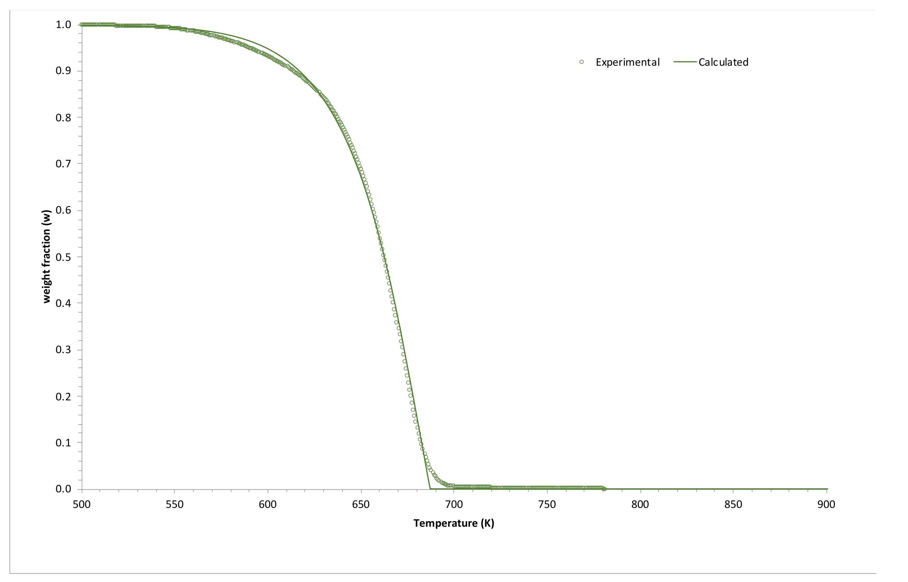
An example can be the decomposition of a simple material, polystyrene (PS), in the thermobalance at one single heating rate. The optimisation of the constants can be performed using any spreadsheet, which usually incorporate optimisation methods such as Flexible Simplex [34]. Other programming tools can, of course, also be used for that purpose. Figure 5 shows the fitting obtained, with the following kinetic constant values: k0 = 1.7·10−2 s−1, E/R = 13,200 K, n = 0.86. The spreadsheet used for this calculation is available in the Supplementary Material of this publication (Spreasheet2: PS_kinetics_fitting.odt).
3. Numerical Methods for Complex Materials
3.1. Theoretical Background
For complex materials, using a single step during the decomposition cannot explain the experimental results. Materials that are widely known to behave this way include all kinds of biomass feedstocks, with the initial material composed of cellulose, hemicellulose and lignin [7,35,36].
In the case of materials presenting more than one process during their thermal decomposition, the models will need to include more than one fraction able to decompose into the raw material. This is the case of several materials studied in our department, including plastics such as PET or nylon [37], different rubbers [14] and tires [28], electric wires [38], biomasses such as almond shells or olive stones [35], and sewage sludges [30].
Calculating the kinetic parameters corresponding to lignocellulosic materials implies knowing the reaction mechanisms. Biomass components (lignin, cellulose and hemicellulose) are usually studied separately. Two or three peaks usually appear during the decomposition of such materials; they are usually attributed t hemicellulose (the first process of decomposition, centred at about 250 °C), cellulose (second peak, approximately 380 °C) and lignin (with a very large peak centred at ≈400 °C) [35]. This would indicate that the different fractions’ identity is somewhat maintained, despite the presence of some interactions.
Other materials that present this behaviour are rubbers and tires. TG curves show that three different fractions exist in a raw tire, corresponding to the oil used as plasticizer (the first process observed), natural rubber (NR, second peak), and styrene-butadiene rubber (SBR, third process). A study was performed and it confirmed the presence of these three fractions in the decomposition, based on a mass spectrometry analysis of the gases that had evolved during the decomposition [31].
Sewage sludge thermal decomposition also takes place through a mechanism involving three fractions. In this case, the fractions were associated with dead bacteria, biodegradable organic matter and non-biodegradable compounds [30].
Generally, we can consider a number of reactions similar to that shown in (S1), therefore:
where Fi is the ‘i’ fraction of the material, Gi the gases produced by this fraction, Si the solid residue, and si the yield coefficient of the solid fraction, fio is the contribution of each fraction to the weight of the initial sample, and therefore:
For each of the material’s ‘f’ fractions, the decomposition rate given by Equation (4) will generally be:
The initial condition of this equation is wi = 0 for t = 0, for every fraction. The weight of each fraction t each time was calculated as follows:
The total weight, each time, was calculated as follows:
Some materials are composed of a carbonaceous or inert fraction that does not decompose under experimental conditions. In this case, for this fraction, and during all runs, so the contribution to the weight was fi0.
3.2. Simulations and Application to Some Materials
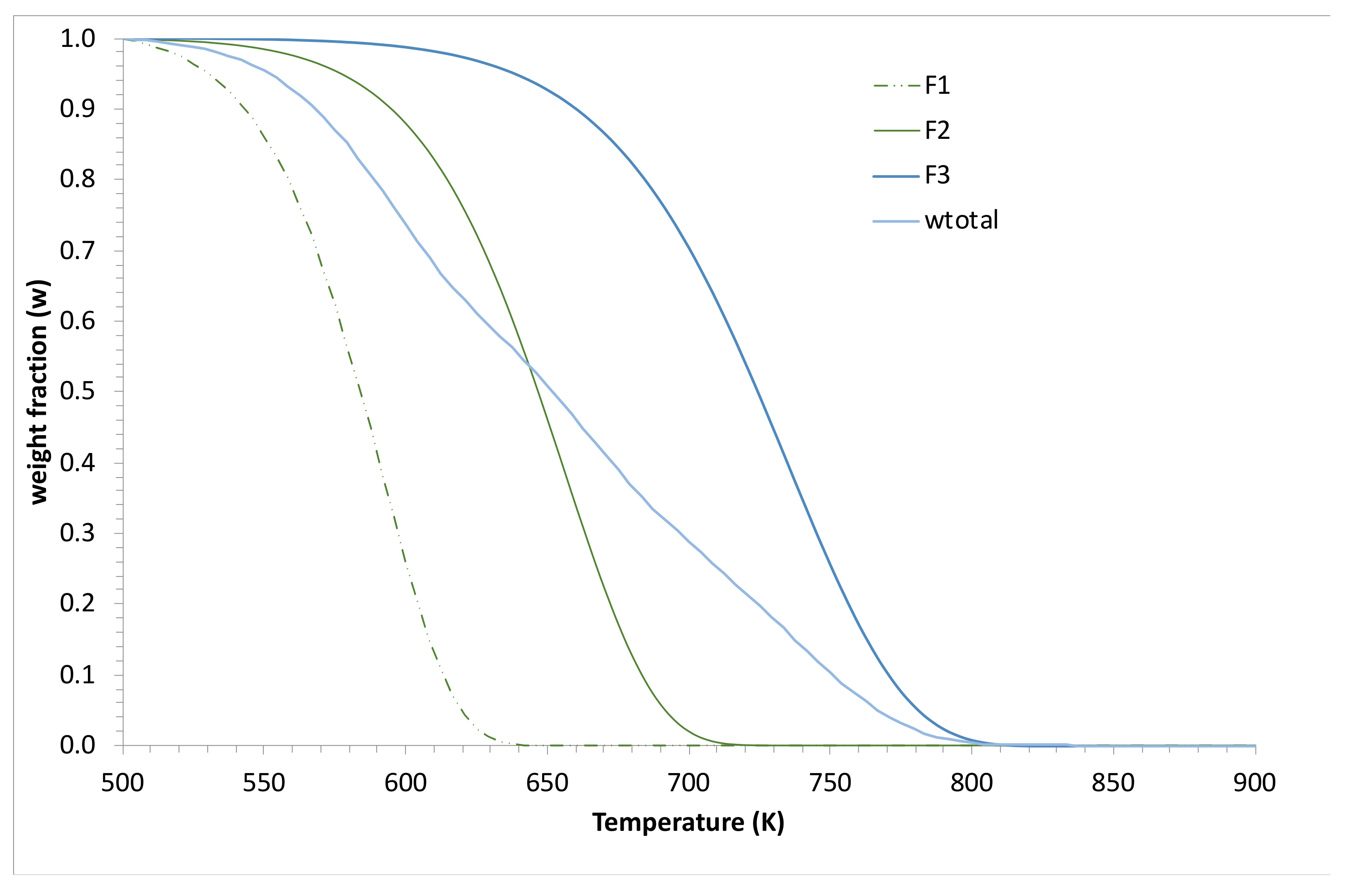
Furthermore, by simulating the decomposition, the method allows visualising how the decomposition of each initial organic fraction evolves with temperature. Figure 6 shows an example, obtained with the following constants: k01 = 107 s−1, E1/R = 12,500 K, n1 = 1; k02 = 106 s−1, E2/R = 12,500 K, n1 = 1; k03 = 105 s−1, E1/R = 12,500 K, n3 = 1; fi0 = 0.3; f20 = 0.3.
The number of optimisation parameters is f × ki0, f × (Ei/R), f × ni, and (f − 1) values of fi0, i.e., a total of (4f − 1). This number is commonly within the 7–15 range, which is low compared to the usual number of points fitted using the method, implying that there would be no compensation effect.
4. Comparison with Other Methods
Most kinetic analysis methods that consider the data of more than one HR are based on the concept of Tf. This temperature is the one at which an equivalent (fixed) state of transformation is achieved at the different HRs. Several different explicit relations between the Tf and the heating rate are proposed, but the vast majority present an equation similar to [40]:
Here, the heating rate ‘β’ is used, instead of the actual T = f(t). The representation of the natural logarithm vs. 1/Tf at the different HRs would give a straight line with a slope equal to (−E/R).
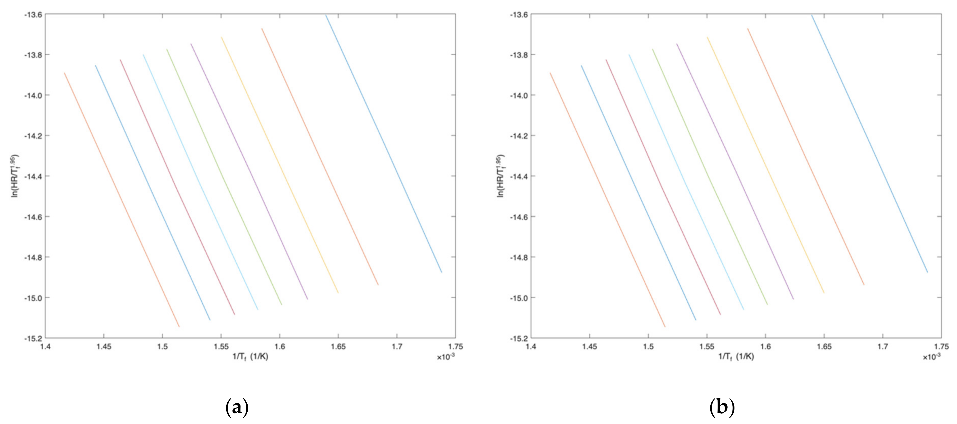
We verified the method’s robustness. To do so, the values of Tf at w = 0.9, 0.8, 0.7, 0.6, 0.5, 0.4, 0.3, 0.2 and 0.1 were extracted from the simulated data presented in Figure 1 corresponding to k1 and E1/R (equal to 12,500 K). In this case, an Octave programme was used for simplicity. Worthy of note, the experimental errors were avoided because the data was simulated by numerical integration of the differential equation. Figure 8a shows the lines obtained for the different values of fixed ‘w’. As can be observed, the lines are straight, and the slope of the plots give an average value of E/R = 12,790 K, that is, an error of +2.32% was calculated. Let us try other values of constants, for example those corresponding to Figure 4, i.e., k0 = 1026 s−1, E/R = 48,100 K, n = 1. Figure 8b shows the resulting plot. For these parameters, a value of E/R = 51,188 K is obtained, representing an error of +6.48%.
The errors generated by these methods are clearly rather substantial. Thus, as a general rule, these methods should be avoided. They do provide a good starting point to determine the E/R but they should never be considered as definitive. Furthermore, in many cases, the calculation of k0 is overlooked. Naturally, the (previously mentioned) methods, that do not even consider curves obtained at different HRs, are even worse.
Different authors have pointed to the inaccuracy of integral and/or differential methods. Marcilla and Beltran [41] applied the Friedman method to the decomposition of PVC, and illustrated the need to precisely select the state of decomposition when comparing the different curves. They showed that the calculation results were very much dependent on the procedure that was followed to select the points.
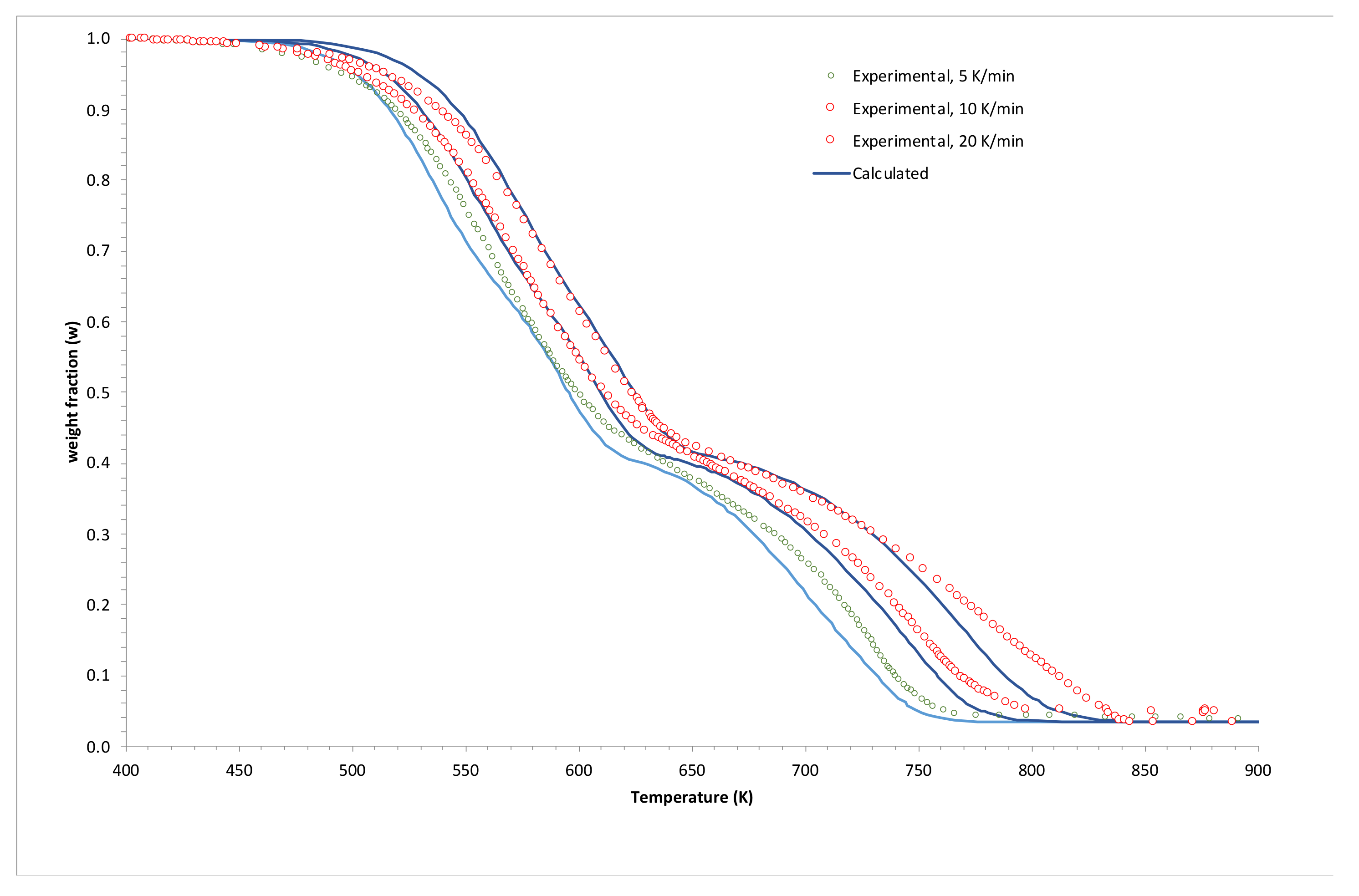
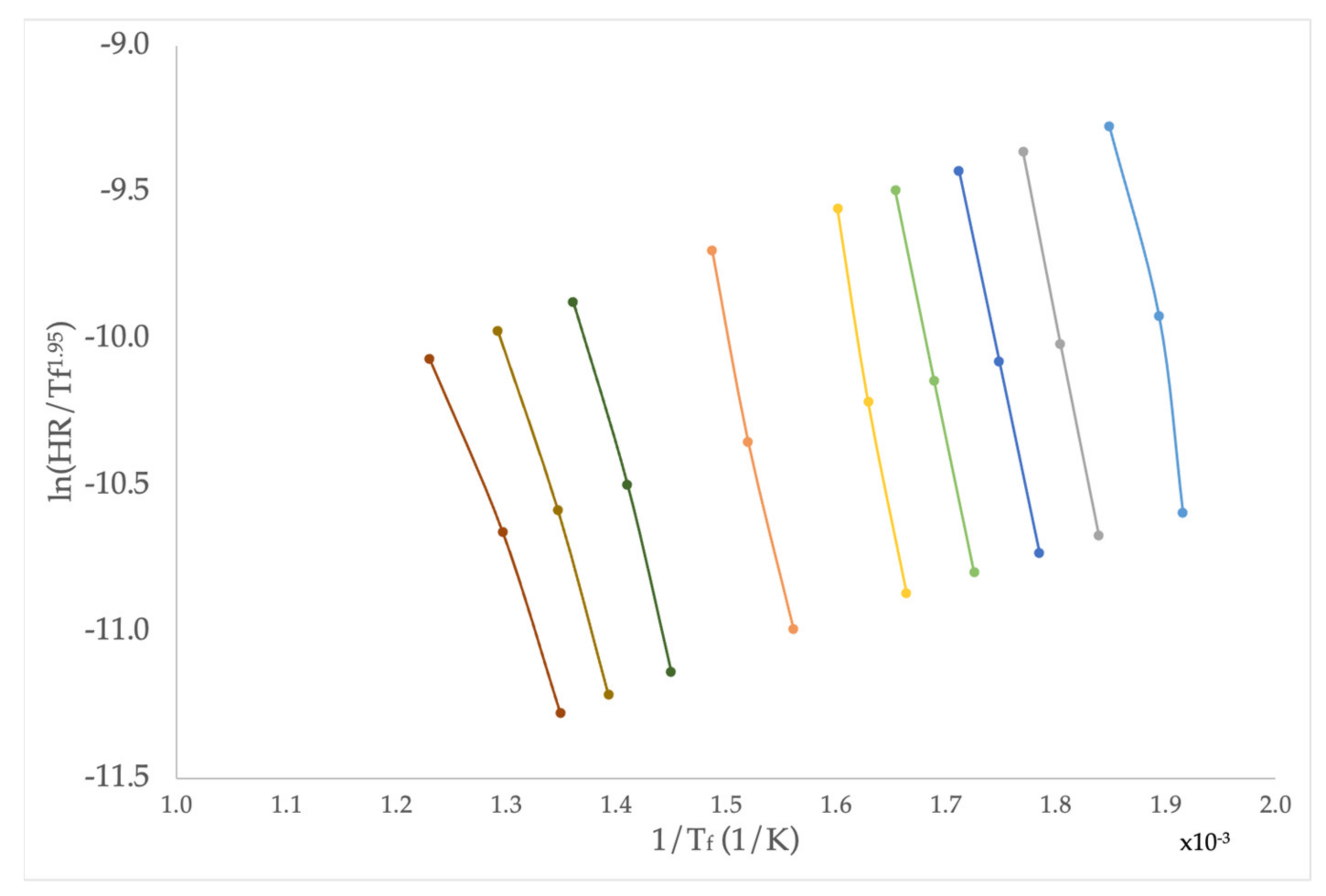
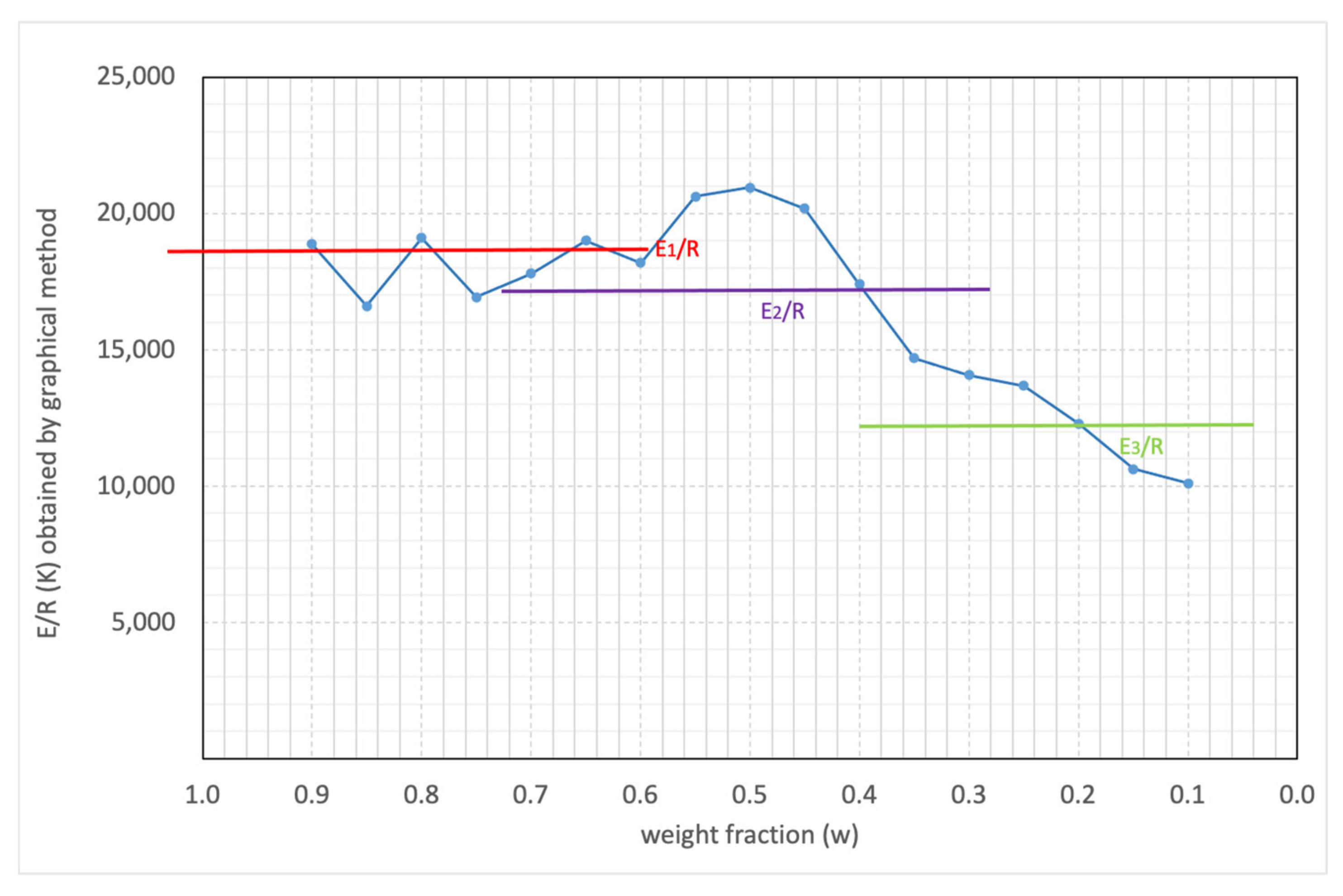
The use of Equation (13) was also tested using data measured at our lab. A more complex material, coffee husks, was selected, the decomposition of which is detailed above (Figure 7). The different Tf values were also calculated with w values ranging from 0.9 to 0.1. Figure 9 shows the results, with an average value of E/R = 16,231 K. We must remember that the method is unable to propose a reaction scheme comprising more than one initial fraction. Values E1/R = 17,673 K, E2/R = 11,919 K and E3/R = 12,566 K were found using numerical integration and optimisation. A considerable error is committed when using simplified methods. Figure 10 shows all activation energy (E/R) values calculated, applying the py-isoconversion method [40] and using Equation (13). For comparison purposes, we plotted the values of E/R obtained by numerical integration and optimisation. As we can observe, the E/R values are similar, but it is not possible to distinguish, using graphical methods, the different organic fractions contained in the husks.
5. Conclusions
This work shows in detail how to use numerical methods to kinetically fit the experimental data obtained in a thermobalance. Examples on the application of the method to the decomposition of PE, nylon, sewage sludges and coffee husks are given.
The importance of using the temperature measured by the analytical equipment for the kinetic fit of the data is highlighted. Methods using the programmed temperature are discussed.
Furthermore, the importance of considering various experimental conditions when performing kinetic analysis is shown, and it is shown that a single TG curve should never be used for this purpose. In this way, PE decomposition is easily fitted to three different models without significative differences, if only one curve is considered.
The numerical method for the fitting of several curves obtained at different heating rates is compared with isoconversional methods, showing that the precision of the latter is not adequate for the fit of complex curves. By applying isoconversional methods to the decomposition of coffee husks, a great error in the calculation of activation energies is shown, other than that method does not permit to distinguish the different fractions present in the original material.
Supplementary Materials
The following are available online at https://0-www-mdpi-com.brum.beds.ac.uk/article/10.3390/thermo1010003/s1, Spreadsheet 1: “Simulations of weight loss curves.ods”; Spreadsheet 2: “PS_kinetics_fitting.ods”.
Funding
This research was funded by the Ministerio de Ciencia e Innovación (Spain’s Ministry of Science and Innovation), grant number PID2019-105359RB-I00 and the UAUSTI20-05 grant from the University of Alicante (Spain).
Institutional Review Board Statement
Not applicable.
Informed Consent Statement
Not applicable.
Data Availability Statement
The datasets generated and/or analysed in the current study are available upon reasonable request to the corresponding author.
Conflicts of Interest
The authors declare no conflict of interest.
References
- Freeman, E.S.; Carroll, B. The application of thermoanalytical techniques to reaction kinetics. The thermogravimetric evaluation of the kinetics of the decomposition of calcium oxalate monohydrate. J. Phys. Chem. 1958, 62, 394–397. [Google Scholar] [CrossRef]
- Simons, E.L.; Newkirk, A.E.; Aliferis, I. Performance of a pen-recording chevenard thermobalance. Anal. Chem. 1957, 29, 48–54. [Google Scholar] [CrossRef]
- Horowitz, H.H.; Metzger, G. A new analysis of thermogravimetric traces. Anal. Chem. 1963, 35, 1464–1468. [Google Scholar] [CrossRef]
- Coats, A.W.; Redfern, J.P. Kinetic parameters from thermogravimetric data. Nature 1964, 201, 68–69. [Google Scholar] [CrossRef]
- Friedman, H.L. Kinetics of thermal degradation of char-forming plastics from thermogravimetry. Application to a phenolic plastic. J. Polym. Sci. Part C 2007, 6, 183–195. [Google Scholar] [CrossRef]
- Conesa, J.A.A.; Marcilla, A.; Font, R.; Caballero, J.A.A. Thermogravimetric studies on the thermal decomposition of polyethylene. J. Anal. Appl. Pyrolysis 1996, 36, 1–15. [Google Scholar] [CrossRef]
- Conesa, J.A.A.; Caballero, J.A.; Marcilla, A.; Font, R. Analysis of different kinetic models in the dynamic pyrolysis of cellulose. Thermochim. Acta 1995, 254, 175–192. [Google Scholar] [CrossRef]
- Agrawal, R.K. Analysis of irreversible complex chemical reactions and some observations on their overall activation energy. Thermochim. Acta 1988, 128, 185–208. [Google Scholar] [CrossRef]
- Ferrer, J.A.C. Curso Básico de Ánalisis Térmico: Termogravimetría, Cinética de Reacciones y Análisis Térmico Diferencial; Editorial Club Universitario: Alicante, Spain, 2000; ISBN 84-8454-018-9. [Google Scholar]
- Islamova, S.I.; Timofeeva, S.S.; Khamatgalimov, A.R.; Ermolaev, D.V. Kinetic analysis of the thermal decomposition of lowland and high-moor peats. Solid Fuel Chem. 2020, 54, 154–162. [Google Scholar] [CrossRef]
- Reinehr, T.O.; Ohara, M.A.; de Oliveira Santos, M.P.; Barros, J.L.M.; Bittencourt, P.R.S.; Baraldi, I.J.; da Silva, E.A.; Zanatta, E.R. Study of pyrolysis kinetic of green corn husk. J. Therm. Anal. Calorim. 2020, 1–12. [Google Scholar] [CrossRef]
- Salin, I.M.; Seferis, J.C. Kinetic analysis of high-resolution TGA variable heating rate data. J. Appl. Polym. Sci. 1993, 47, 847–856. [Google Scholar] [CrossRef]
- Fetisova, O.Y.; Kuznetsov, P.N.; Chesnokov, N.V. Kinetic study of the thermal decomposition of low-ranked coal of Mongolia and Tuva. Chem. Sustain. Dev. 2019. [Google Scholar] [CrossRef]
- Conesa, J.A.; Marcilla, A. Kinetic study of the thermogravimetric behavior of different rubbers. J. Anal. Appl. Pyrolysis 1996, 37, 95–110. [Google Scholar] [CrossRef]
- Conesa, J.A.; Font, R.; Marcilla, A. Gas from the pyrolysis of scrap tires in a fluidized bed reactor. Energy Fuels 1996, 10, 134–140. [Google Scholar] [CrossRef]
- Várhegyi, G.; Czégény, Z.; Jakab, E.; McAdam, K.; Liu, C. Tobacco pyrolysis. Kinetic evaluation of thermogravimetric-mass spectrometric experiments. J. Anal. Appl. Pyrolysis 2009, 86, 310–322. [Google Scholar] [CrossRef] [Green Version]
- Grønli, M.G.; Várhegyi, G.; Di Blasi, C. Thermogravimetric analysis and devolatilization kinetics of wood. Ind. Eng. Chem. Res. 2002, 41, 4201–4208. [Google Scholar] [CrossRef]
- Vyazovkin, S.; Wight, C.A. Model-free and model-fitting approaches to kinetic analysis of isothermal and nonisothermal data. Thermochim. Acta 1999, 340–341, 53–68. [Google Scholar] [CrossRef]
- Font, R.; García, A.N. Application of the transition state theory to the pyrolysis of biomass and tars. J. Anal. Appl. Pyrolysis 1995, 35, 249–258. [Google Scholar] [CrossRef]
- Di Blasi, C. Linear pyrolysis of cellulosic and plastic waste. J. Anal. Appl. Pyrolysis 1997, 40–41, 463–479. [Google Scholar] [CrossRef]
- Baker, R.R. Kinetic mechanism of the thermal decomposition of tobacco. Thermochim. Acta 1979, 28, 45–57. [Google Scholar] [CrossRef]
- Ortega, A. The kinetics of solid-state reactions toward consensus, Part 2: Fitting kinetics data in dynamic conventional thermal analysis. Int. J. Chem. Kinet. 2002, 34, 193–208. [Google Scholar] [CrossRef]
- Gao, X.; Chen, D.; Dollimore, D. The correlation between the value of α at the maximum reaction rate and the reaction mechanisms. A theoretical study. Thermochim. Acta 1993, 223, 75–82. [Google Scholar] [CrossRef]
- Agrawal, R.K. Compensation effect in the pyrolysis of cellulosic materials. Thermochim. Acta 1985, 90, 347–351. [Google Scholar] [CrossRef]
- Chornet, E.; Roy, C. Compensation effect in the thermal decomposition of cellulosic materials. Thermochim. Acta 1980, 35, 389–393. [Google Scholar] [CrossRef]
- Caballero, J.A.; Conesa, J.A. Mathematical considerations for nonisothermal kinetics in thermal decomposition. J. Anal. Appl. Pyrolysis 2005, 73, 85–100. [Google Scholar] [CrossRef]
- Edwin, K.P.; Chong, S.H.Z. An Introduction to Optimization, 4th ed.; Wiley and Sons: Hoboken, NJ, USA, 2013; Available online: https://0-www-wiley-com.brum.beds.ac.uk/en-us/An+Introduction+to+Optimization%2C+4th+Edition-p-9781118515150 (accessed on 18 January 2021).
- Conesa, J.A.A.; Font, R.; Fullana, A.; Caballero, J.A.A. Kinetic model for the combustion of tyre wastes. Fuel 1998, 77, 1469–1475. [Google Scholar] [CrossRef]
- Font, R.; Marcilla, A.; Garcia, A.N.; Caballero, J.A.; Conesa, J.A. Kinetic models for the thermal degradation of heterogeneous materials. J. Anal. Appl. Pyrolysis 1995, 32, 29–39. [Google Scholar] [CrossRef]
- Conesa, J.A.A.; Marcilla, A.; Prats, D.; Rodriguez-Pastor, M. Kinetic study of the pyrolysis of sewage sludge. Waste Manag. Res. 1997, 15, 293–305. [Google Scholar] [CrossRef]
- Conesa, J.A.; Font, R.; Marcilla, A. Mass spectrometry validation of a kinetic model for the thermal decomposition of tyre wastes. J. Anal. Appl. Pyrolysis 1997, 43, 83–96. [Google Scholar] [CrossRef]
- Koga, N.; Šesták, J.; Málek, J. Distortion of the Arrhenius parameters by the inappropriate kinetic model function. Thermochim. Acta 1991, 188, 333–336. [Google Scholar] [CrossRef]
- Várhegyi, G.; Antal, M.J.; Jakab, E.; Szabó, P. Kinetic modeling of biomass pyrolysis. J. Anal. Appl. Pyrolysis 1997, 42, 73–87. [Google Scholar] [CrossRef] [Green Version]
- Nelder, J.A.; Mead, R. A simple method for function minimization. Comput. J. 1965, 7, 308–313. [Google Scholar] [CrossRef]
- Caballero, J.A.A.; Conesa, J.A.A.; Font, R.; Marcilla, A. Pyrolysis kinetics of almond shells and olive stones considering their organic fractions. J. Anal. Appl. Pyrolysis 1997, 42, 159–175. [Google Scholar] [CrossRef]
- Varhegyi, G.; Antal Jr, M.J.; Szekely, T.; Szabo, P. Kinetics of the thermal decomposition of cellulose, hemicellulose, and sugar cane bagasse. Energy Fuels 1989, 3, 329–335. [Google Scholar] [CrossRef]
- Iñiguez, M.E.; Conesa, J.A.; Fullana, A. Pollutant content in marine debris and characterization by thermal decomposition. Mar. Pollut. Bull. 2017. [Google Scholar] [CrossRef] [Green Version]
- Conesa, J.A.; Moltó, J.; Font, R.; Egea, S. Polyvinyl chloride and halogen-free electric wires thermal decomposition. Ind. Eng. Chem. Res. 2010, 49, 11841–11847. [Google Scholar] [CrossRef]
- Conesa, J.A.; Sánchez, N.E.; Garrido, M.A.; Casas, J.C. Semivolatile and volatile compound evolution during pyrolysis and combustion of Colombian coffee husk. Energy Fuels 2016, 30, 7827–7833. [Google Scholar] [CrossRef] [Green Version]
- Starink, M.J. The determination of activation energy from linear heating rate experiments: A comparison of the accuracy of isoconversion methods. Thermochim. Acta 2003, 404, 163–176. [Google Scholar] [CrossRef] [Green Version]
- Marcilla, A.; Beltrán, M. Thermogravimetric kinetic study of poly(vinyl chloride) pyrolysis. Polym. Degrad. Stab. 1995, 48, 219–229. [Google Scholar] [CrossRef]
Figure 1.
Effect of activation energy and the preexponential factor on the position and shape of the decomposition curve at a fixed heating rate of 10 K/min. Values used in the simulation: k1 = 106 s−1, k2 = 107 s−1, E1/R = 12,500 K, E2/R = 15,000 K.
Figure 1.
Effect of activation energy and the preexponential factor on the position and shape of the decomposition curve at a fixed heating rate of 10 K/min. Values used in the simulation: k1 = 106 s−1, k2 = 107 s−1, E1/R = 12,500 K, E2/R = 15,000 K.
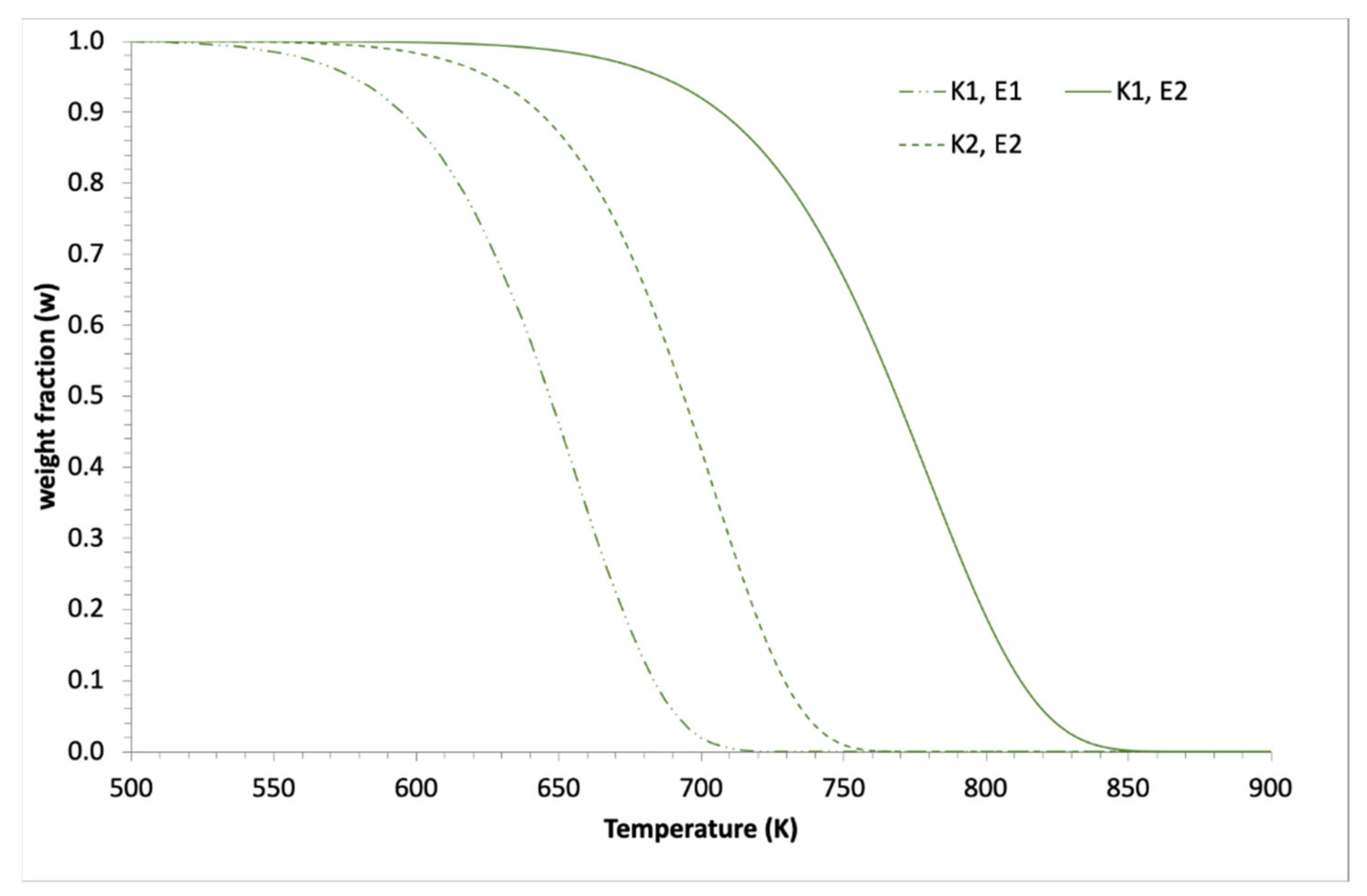
Figure 2.
Effect of the reaction order on the position and shape of the decomposition curve at a fixed heating rate of 10 K/min.
Figure 2.
Effect of the reaction order on the position and shape of the decomposition curve at a fixed heating rate of 10 K/min.
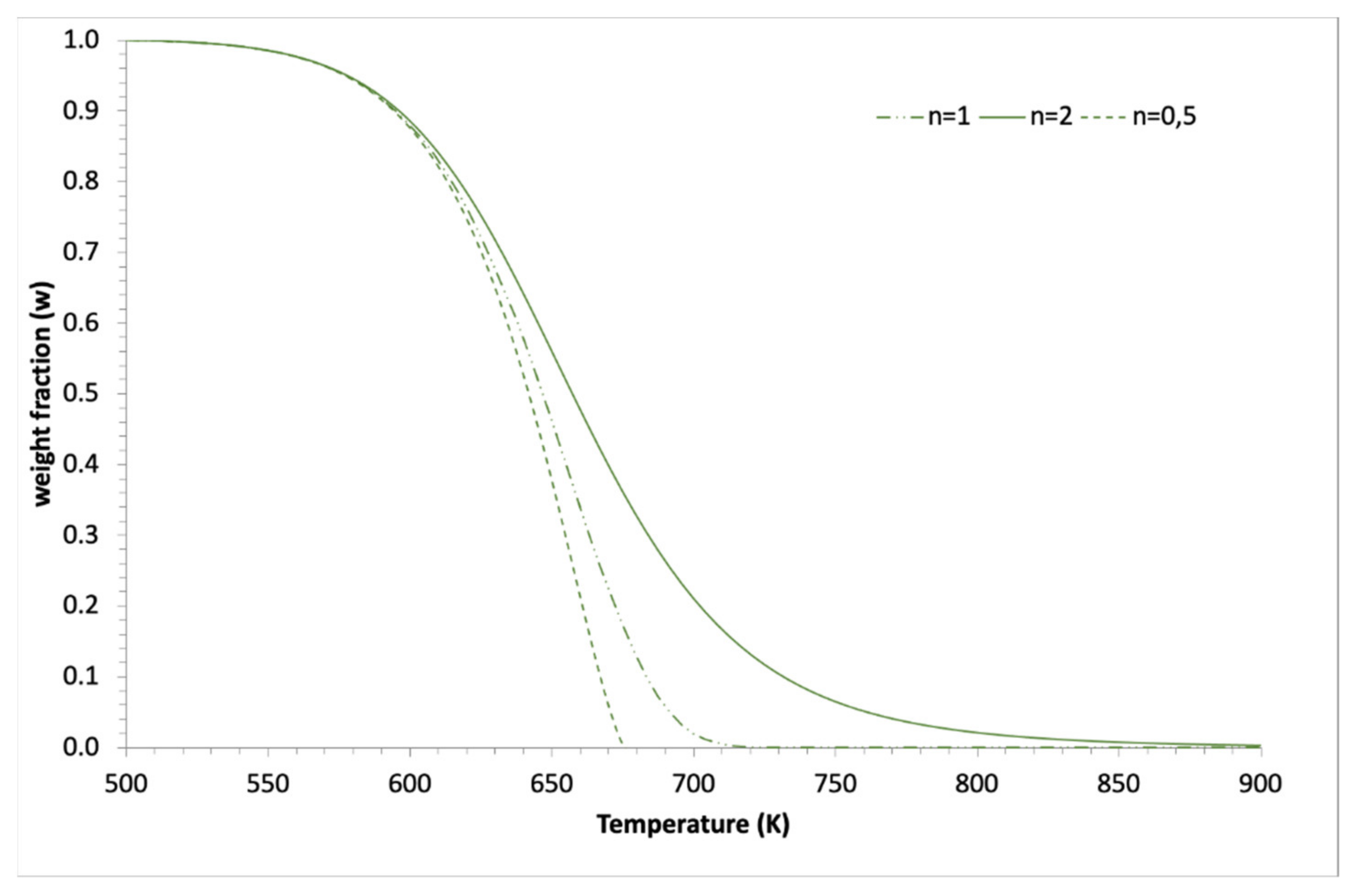
Figure 3.
Effect of the heating rate (HR) on the decomposition curve’s position without varying the kinetic constants. In this case, the curve moves appreciably to the right when the HR increases (in K/min, indicated in the graphics).
Figure 3.
Effect of the heating rate (HR) on the decomposition curve’s position without varying the kinetic constants. In this case, the curve moves appreciably to the right when the HR increases (in K/min, indicated in the graphics).

Figure 4.
Effect of the heating rate (HR) on the decomposition curve’s position without varying the kinetic constants. In this case, the curve does NOT move appreciably to the right when the HR increases (in K/min, indicated in the graphics).
Figure 4.
Effect of the heating rate (HR) on the decomposition curve’s position without varying the kinetic constants. In this case, the curve does NOT move appreciably to the right when the HR increases (in K/min, indicated in the graphics).
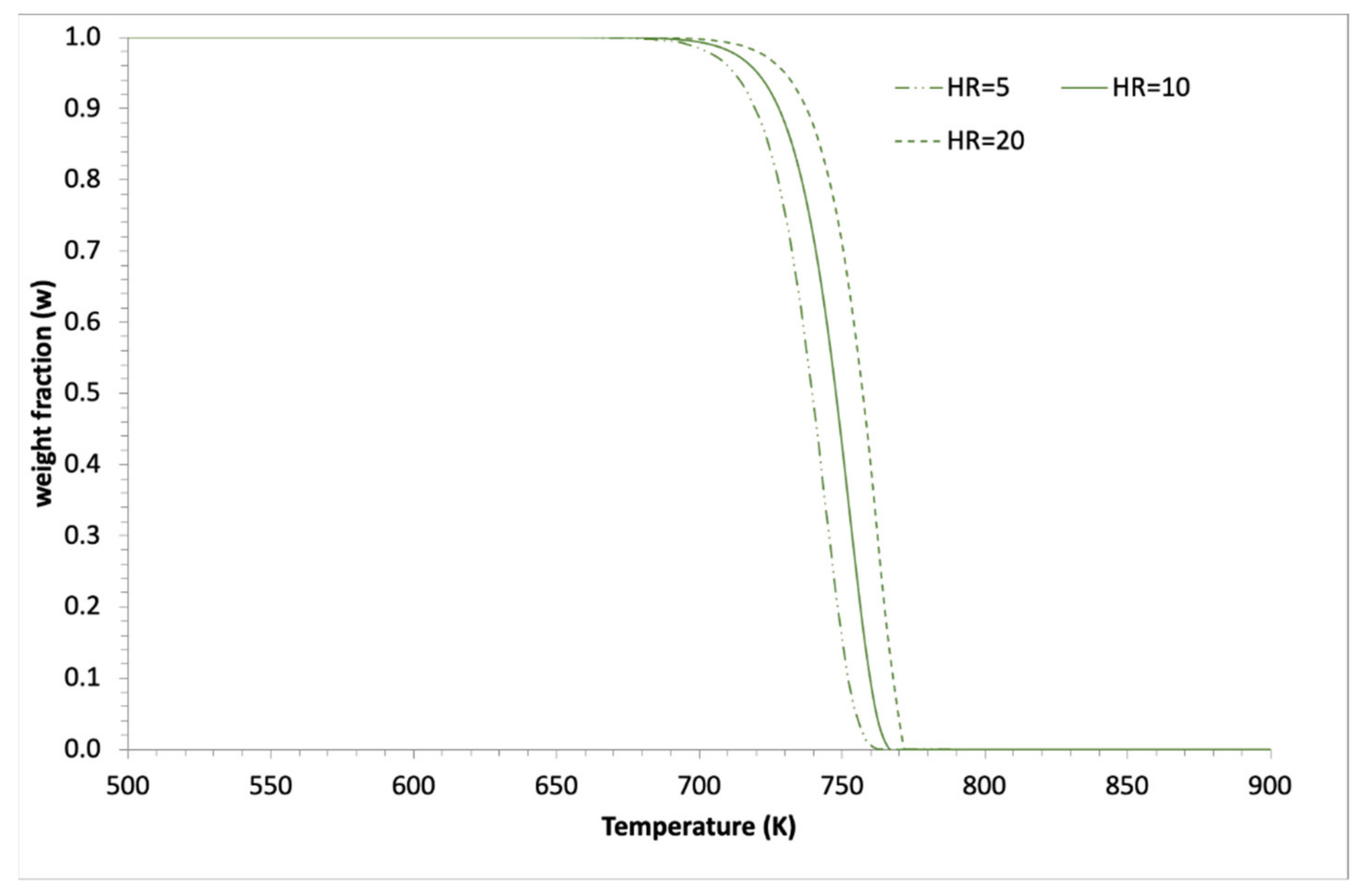
Figure 5.
Thermal decomposition of PS at 10 K/min. Experimental and calculated curve.

Figure 6.
Evolution of the decomposition of three different initial organic fractions (F1, F2 and F3) and total weight loss (wtotal) for the simulation of a run performed at 10 K/min. The values of the kinetic parameters are shown in the main text.
Figure 6.
Evolution of the decomposition of three different initial organic fractions (F1, F2 and F3) and total weight loss (wtotal) for the simulation of a run performed at 10 K/min. The values of the kinetic parameters are shown in the main text.

Figure 7.
Thermal decomposition of coffee husks at three different HR. Experimental and calculated curves (the kinetic parameters values are: k01 = 10.6 s−1, E1/R = 17,673 K, k02 = 7.26 s−1, E2/R = 11,919 K, k03 = 5.1 s−1, E3/R = 12,566 K, f10 = 0.26, f20 = 0.31, all orders were considered equal to 1).

Figure 8.
Plots corresponding to the different values of Tf calculated based on the data in Figure 1 and Figure 4, using as fixed decomposition state of transformation: w = 0.9, 0.8, 0.7, 0.6, 0.5, 0.4, 0.3, 0.2 and 0.1 (the line moves to the right as the level of decomposition increases). (a) simulated with values of k1 and E1 of Figure 1, (b) simulated with data of Figure 4.

Figure 9.
Plots corresponding to the different Tf values calculated for the decomposition of coffee husks (Figure 7), using as fixed decomposition state of transformation w = 0.9, 0.8, 0.7, 0.6, 0.5, 0.4, 0.3, 0.2 and 0.1.
Figure 9.
Plots corresponding to the different Tf values calculated for the decomposition of coffee husks (Figure 7), using as fixed decomposition state of transformation w = 0.9, 0.8, 0.7, 0.6, 0.5, 0.4, 0.3, 0.2 and 0.1.

Figure 10.
Activation energy (E/R) calculated using the py-isoconversional method linearizing differential equation. The E/R values obtained by numerical integration and optimisation were plotted for comparison purposes.
Figure 10.
Activation energy (E/R) calculated using the py-isoconversional method linearizing differential equation. The E/R values obtained by numerical integration and optimisation were plotted for comparison purposes.
Publisher’s Note: MDPI stays neutral with regard to jurisdictional claims in published maps and institutional affiliations. |
© 2021 by the author. Licensee MDPI, Basel, Switzerland. This article is an open access article distributed under the terms and conditions of the Creative Commons Attribution (CC BY) license (http://creativecommons.org/licenses/by/4.0/).
Share and Cite
MDPI and ACS Style
Conesa, J.A. Numerical Integration of Weight Loss Curves for Kinetic Analysis. Thermo 2021, 1, 32-44. https://0-doi-org.brum.beds.ac.uk/10.3390/thermo1010003
AMA Style
Conesa JA. Numerical Integration of Weight Loss Curves for Kinetic Analysis. Thermo. 2021; 1(1):32-44. https://0-doi-org.brum.beds.ac.uk/10.3390/thermo1010003
Chicago/Turabian StyleConesa, Juan A. 2021. "Numerical Integration of Weight Loss Curves for Kinetic Analysis" Thermo 1, no. 1: 32-44. https://0-doi-org.brum.beds.ac.uk/10.3390/thermo1010003