Assessing the Potential of Artificial Intelligence (Artificial Neural Networks) in Predicting the Spatiotemporal Pattern of Wildfire-Generated PM2.5 Concentration


Abstract
:1. Introduction
2. Materials and Methods
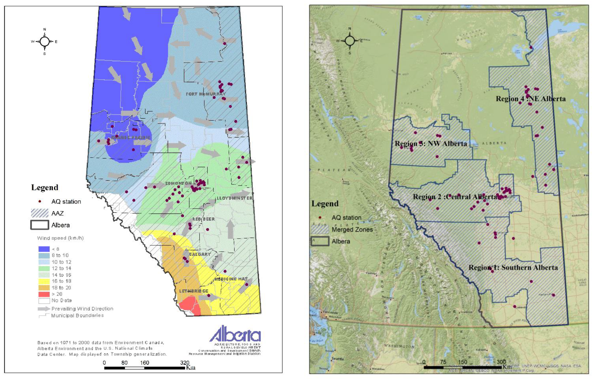
2.1. Study Domain and Period
2.2. Data
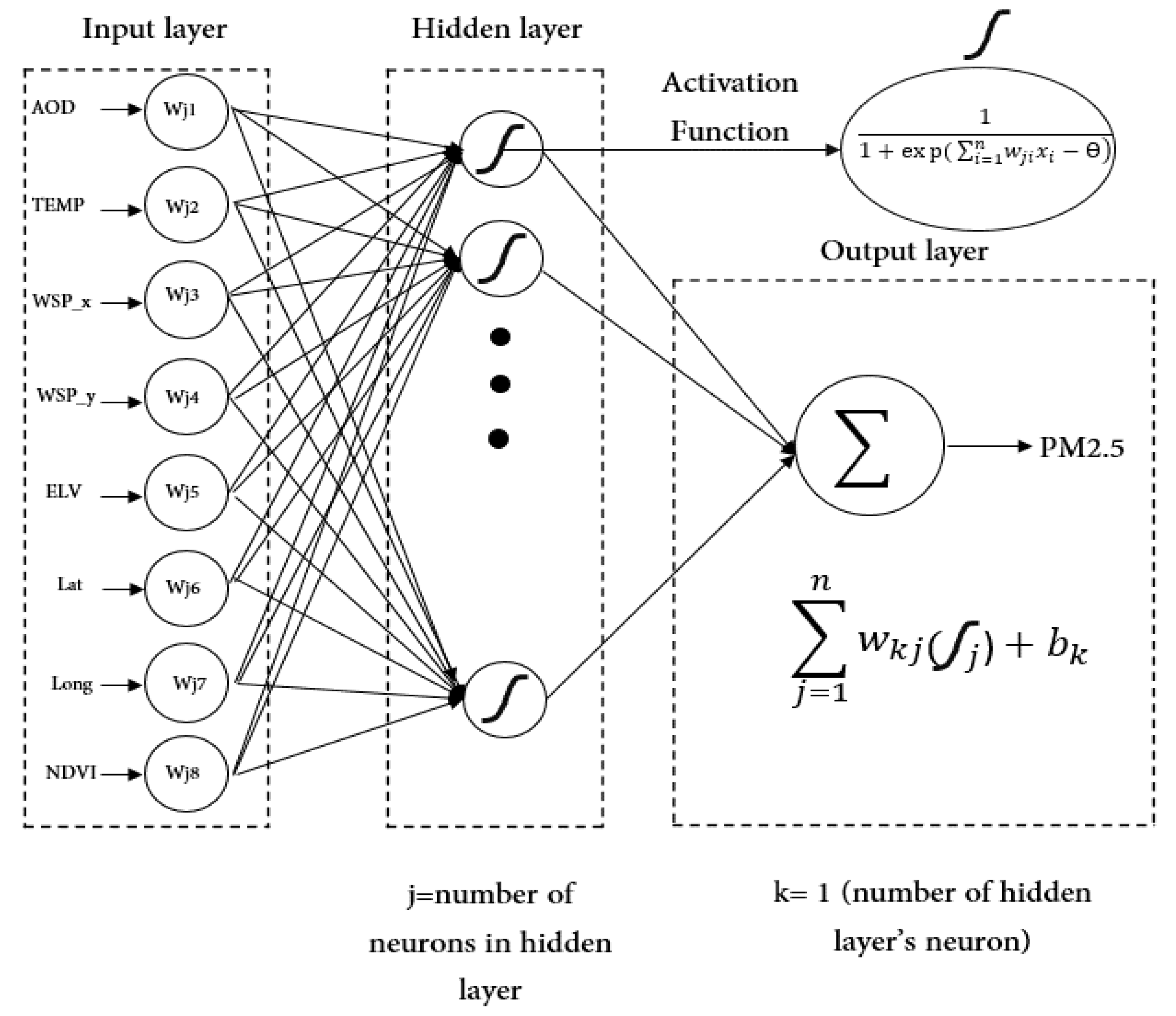
2.3. Methods
3. Results
3.1. Descriptive Statistics
3.2. ANN Implementation Process
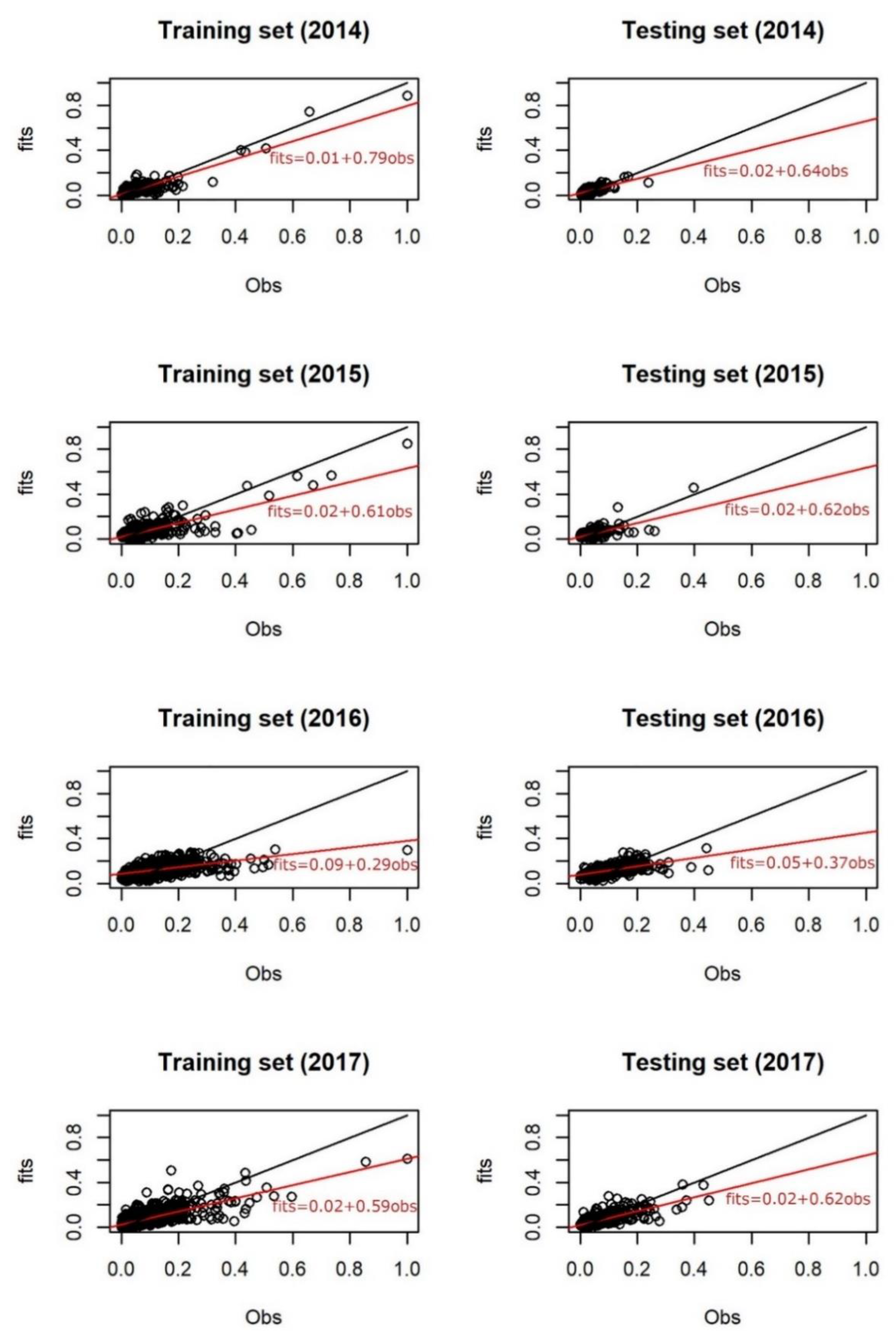
3.3. MLR Models and Temporal ANN Results
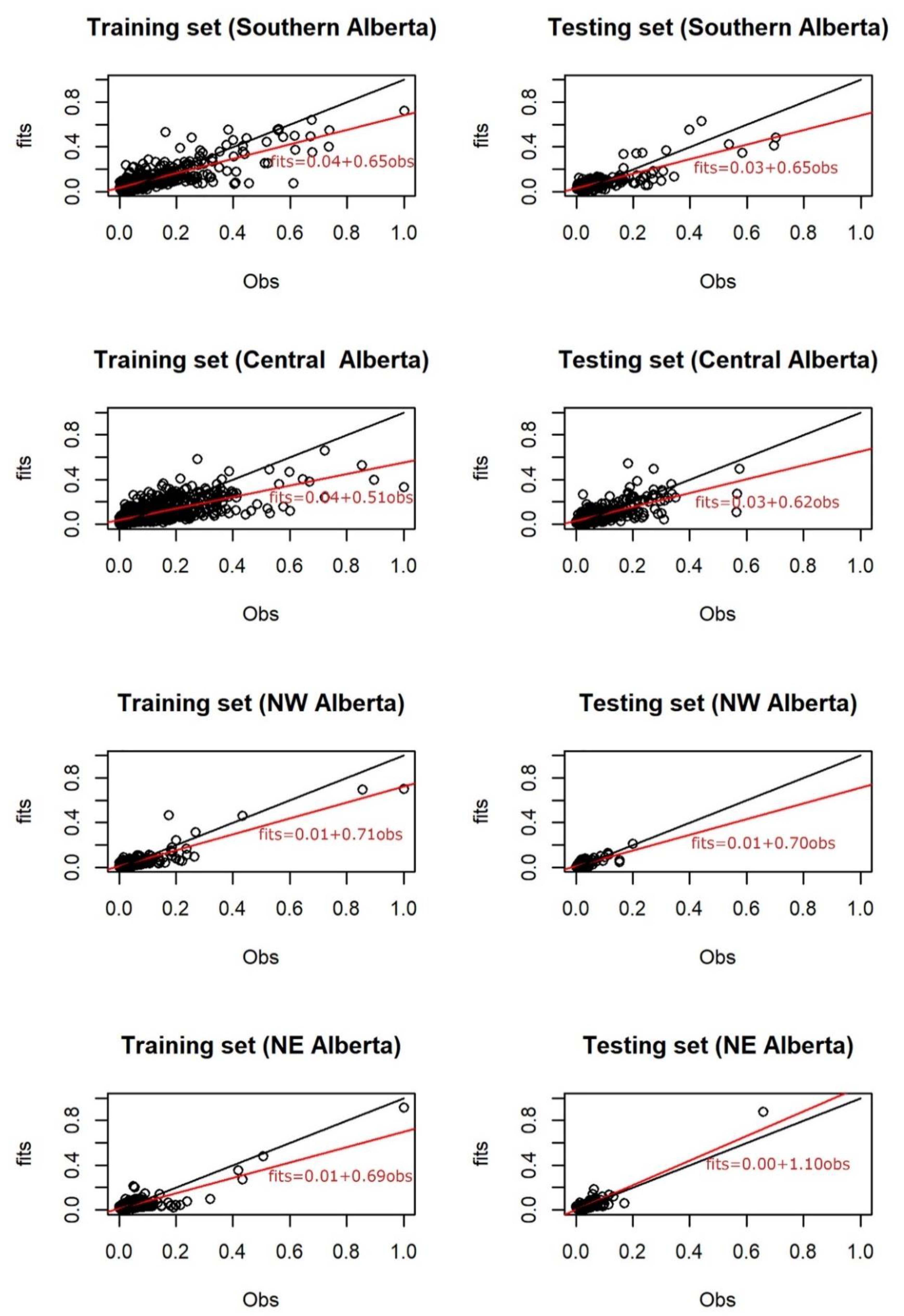
3.4. Spatial ANN Results
3.5. Validation of Temporal ANN Predictions
4. Discussion
4.1. Temporal and Spatial Prediction
4.2. Limitations
5. Conclusions
Author Contributions
Funding
Data Availability Statement
Acknowledgments
Conflicts of Interest
References
- Youssouf, H.C.; Roblou, L.L.; Assamoi, E.M.; Salonen, R.O.; Maesano, C. Quantifying Wild Fi Res Exposure for Investigating Health-Related Effects. Atmos. Environ. 2014, 97, 239–251. [Google Scholar] [CrossRef]
- World Health Organization. Wildfire Smoke a Guide for Public Health Officials. 2016. Available online: https://www3.epa.gov/airnow/wildfire_may2016.pdf (accessed on 6 January 2021).
- Black, C.; Tesfaigzi, Y.; Bassein, J.A.; Miller, L.A. Wild Fi Re Smoke Exposure and Human Health: Signi Fi Cant Gaps in Research for a Growing Public Health Issue. Environ. Toxicol. Pharmacol. 2017, 55, 186–195. [Google Scholar] [CrossRef]
- Cascio, W.E. Wildland Fire Smoke and Human Health. Sci. Total Environ. 2018, 624, 586–595. [Google Scholar] [CrossRef]
- Liu, J.C.; Pereira, G.; Uhl, S.A.; Bravo, M.A.; Bell, M.L. A Systematic Review of the Physical Health Impacts from Non-Occupational Exposure to Wild Fi Re Smoke. Environ. Res. 2015, 136, 120–132. [Google Scholar] [CrossRef] [Green Version]
- Lv, B.; Hu, Y.; Chang, H.H.; Russell, A.G.; Cai, J.; Xu, B.; Bai, Y. Daily Estimation of Ground-Level PM2.5 Concentrations at 4 km Resolution over Beijing-Tianjin-Hebei by Fusing MODIS AOD and Ground Observations. Sci. Total Environ. 2017, 580, 235–244. [Google Scholar] [CrossRef]
- Zheng, Y.; Zhang, Q.; Liu, Y.; Geng, G.; He, K. Estimating Ground-Level PM2.5concentrations over Three Megalopolises in China Using Satellite-Derived Aerosol Optical Depth Measurements. Atmos. Environ. 2016, 124, 232–242. [Google Scholar] [CrossRef]
- Xie, Y.; Wang, Y.; Zhang, K.; Dong, W.; Lv, B.; Bai, Y. Daily Estimation of Ground-Level PM2.5 Concentrations over Beijing Using 3 Km Resolution MODIS AOD. Environ. Sci. Technol. 2015, 49, 12280–12288. [Google Scholar] [CrossRef] [Green Version]
- Chudnovsky, A.A.; Koutrakis, P.; Kloog, I.; Melly, S.; Nordio, F.; Lyapustin, A.; Wang, Y.; Schwartz, J. Fine Particulate Matter Predictions Using High Resolution Aerosol Optical Depth (AOD) Retrievals. Atmos. Environ. 2014, 89, 189–198. [Google Scholar] [CrossRef] [Green Version]
- Chang, H.H.; Hu, X.; Liu, Y. Calibrating MODIS Aerosol Optical Depth for Predicting Daily PM2.5 Concentrations via Statistical Downscaling. J. Expo. Sci. Environ. Epidemiol. 2014, 24, 398–404. [Google Scholar] [CrossRef] [Green Version]
- Chen, B.B.; Sverdlik, L.G.; Imashev, S.A.; Solomon, P.A.; Lantz, J.; Schauer, J.J.; Shafer, M.M.; Artamonova, M.S. Empirical Relationship between Particulate Matter and Aerosol Optical Depth over Northern Tien-Shan, Central Asia. Air Quality. Atmos. Health 2013, 6, 385–396. [Google Scholar] [CrossRef]
- Kloog, I.; Nordio, F.; Coull, B.A.; Schwartz, J. Incorporating Local Land Use Regression and Satellite Aerosol Optical Depth in a Hybrid Model of Spatiotemporal PM2.5 Exposures in the Mid-Atlantic States. Environ. Sci. Technol. 2012, 46, 11913–11921. [Google Scholar] [CrossRef] [Green Version]
- Lee, H.J.; Coull, B.A.; Bell, M.L.; Koutrakis, P. Use of Satellite-Based Aerosol Optical Depth and Spatial Clustering to Predict Ambient PM 2.5 Concentrations. Environ. Res. 2012, 118, 8–15. [Google Scholar] [CrossRef] [Green Version]
- Chudnovsky, A.A.; Lee, H.J.; Kostinski, A.; Kotlov, T.; Koutrakis, P. Prediction of Daily Fine Particulate Matter Concentrations Using Aerosol Optical Depth Retrievals from the Geostationary Operational Environmental Satellite (GOES). J. Air Waste Manag. Assoc. 2012, 62, 1022–1031. [Google Scholar] [CrossRef]
- Lee, H.J.; Liu, Y.; Coull, B.A.; Schwartz, J.; Koutrakis, P. A Novel Calibration Approach of MODIS AOD Data to Predict PM2.5 Concentrations. Atmos. Chem. Phys. 2011, 11, 7991–8002. [Google Scholar] [CrossRef] [Green Version]
- Mirzaei, M.; Bertazzon, S.; Couloigner, I. Estimation of local daily PM2.5 concentration during wildfire episodes: Integrating MODIS AOD with multivariate linear mixed effect (LME) models. Air Quality. Atmos. Health 2020, 13, 173–185. [Google Scholar] [CrossRef]
- Geng, G.; Murray, N.L.; Tong, D.; Joshua, S.; Fu, X.H.; Lee, P.; Meng, X.; Chang, H.H.; Liu, Y. Satellite-Based Daily PM2.5 Estimates during Fire Seasons in Colorado. J. Geophys. Res. 2018, 123, 8159–8171. [Google Scholar] [CrossRef]
- Mirzaei, M.; Bertazzon, S.; Couloigner, I. Modeling Wildfire Smoke Pollution by Integrating Land Use Regression and Remote Sensing Data: Regional Multi-Temporal Estimates for Public Health and Exposure Models. Atmosphere 2018, 9, 335. [Google Scholar] [CrossRef] [Green Version]
- Reid, C.E.; Jerrett, M.; Petersen, M.L.; Gabriele, G.P.; More, P.E.; Tager, I.B.; Ra, S.M.; Balmes, J.R. Spatiotemporal Prediction of Fine Particulate Matter During the 2008 Northern California Wild Fi Res Using Machine Learning. Environ. Sci. Technol. 2015. [Google Scholar] [CrossRef] [PubMed]
- Gardner, M.W.; Dorling, S.R. Artificial neural networks (the multilayer perceptron)—A review of applications in the atmospheric sciences. Atmos. Environ. 1998, 32, 2627–2636. [Google Scholar] [CrossRef]
- Gupta, P.; Christopher, S.A. Particulate Matter Air Quality Assessment Using Integrated Surface, Satellite, and Meteorological Products: 2. A Neural Network Approach. J. Geophys. Res. 2009, 114, 1–14. [Google Scholar] [CrossRef]
- Hu, X.; Belle, J.H.; Meng, X.; Wildani, A.; Waller, L.A.; Strickland, M.J.; Liu, Y. Stimating PM2.5 Concentrations in the Conterminous United States Using the Random Forest Approach. Environ. Sci. Technol. 2017, 51, 6936–6944. [Google Scholar] [CrossRef] [PubMed]
- Tu, J.V. Advantages and disadvantages of using artificial neural networks versus logistic regression for predicting medical outcomes. J. Clin. Epidemiol. 1996, 49, 1225–1231. [Google Scholar] [CrossRef]
- Grivas, G.; Chaloulakou, A.Ã. Artificial neural network models for prediction of PM10 hourly concentrations, in the Greater Area of Athens, Greece. Atmos. Environ. 2006, 40, 1216–1229. [Google Scholar] [CrossRef]
- Hebb, D.O. The Organization of Behavior: A Neuropsychological Theory; John Wiley: New York, NY, USA, 1949. [Google Scholar]
- Shanmuganathan, S. Artificial Neural Network Modelling. In Studies in Computational Intelligence; Springer International Publishing: Cham, Switzerland, 2016; Volume 628. [Google Scholar] [CrossRef]
- Perez, P.; Reyes, J. An Integrated Neural Network Model for PM10 Forecasting. Atmos. Environ. 2006, 40, 2845–2851. [Google Scholar] [CrossRef]
- Ordieres, J.B.; Vergara, E.P.; Capuz, R.S.; Salazar, R.E. Neural Network Prediction Model for Fine Particulate Matter ( PM2.5) on the US e Mexico Border in Rez ( Chihuahua ) El Paso ( Texas ) and Ciudad Jua. Environ. Model. Softw. 2005, 20, 547–559. [Google Scholar] [CrossRef]
- Jiang, D.; Zhang, Y.; Hu, X.; Zeng, Y.; Tan, J.; Shao, D. Progress in Developing an ANN Model for Air Pollution Index Forecast. Atmos. Environ. 2004, 38, 7055–7064. [Google Scholar] [CrossRef]
- Dorling, S.R.; Foxall, R.J.; Mandic, D.P.; Cawley, G.C. Maximum Likelihood Cost Functions for Neural Network Models of Air Quality Data. Atmos. Environ. 2003, 37, 3435–3443. [Google Scholar] [CrossRef]
- Perez, P.; Trier, A.; Reyes, J. Prediction of PM Concentrations Several Hours in Advance Using Neural Networks in Santiago, Chile. Atmos. Environ. 2000, 34, 1189–1196. [Google Scholar] [CrossRef]
- Comrie, A.C. Comparing Neural Networks and Regression Models for Ozone Forecasting. J. Air Waste Manag. Assoc. 1997, 47, 653–663. [Google Scholar] [CrossRef]
- AAC Alberta Airsheds Council. 2006. Available online: https://www.albertaairshedscouncil.ca/ (accessed on 6 January 2021).
- ACIS. Agroclimatic Atlas Map for Wind Speed, Data Provided by Alberta Agriculture and Forestry. 2019. Available online: https://agriculture.alberta.ca/acis (accessed on 29 December 2020).
- NEO. NEO, Nasa Earth Observations. 2017. Available online: https://neo.sci.gsfc.nasa.gov/view.php?datasetId=MODAL2_D_AER_OD&date=2018-08-01 (accessed on 6 January 2021).
- DMTI. The Gold Standard Canada’s Most Complete and Accurate Mapping Data, DMTI Spatial. 2010. Available online: https://www.dmtispatial.com/ (accessed on 22 August 2018).
- Lary, D.J.; Faruque, F.S.; Malakar, N.; Moore, A.; Roscoe, B.; Adams, Z.L.; Eggelston, Y. Estimating the global abundance of ground level presence of particulate matter (PM2.5). Geospat Health 2014, 8, 611–630. [Google Scholar] [CrossRef]
- May, R.; Dandy, G.; Maier, H. Review of Input Variable Selection Methods for Artificial Neural Networks. In Artificial Neural Networks—Methodological Advances and Biomedical Applications; InTech: London, UK, 2011; pp. 19–44. [Google Scholar] [CrossRef] [Green Version]
- R Core Team. R: A Language and Environment for Statistical Computing; R Foundation for Statistical Computing: Vienna, Austria, 2019. [Google Scholar]
- Riedmiller, M.A.; Braun, H. A direct adaptive method for faster backpropagation learning: The RPROP algorithm. In Proceedings of the IEEE International Conference on Neural Networks, San Francisco, CA, USA, 28 March–1 April 1993; Volume 1, pp. 586–591. [Google Scholar]


| Var. | Min | Mean | Max | SD | Min | Mean | Max | SD | ||
|---|---|---|---|---|---|---|---|---|---|---|
| 2014 (N = 630) | PM2.5 | 0.15 | 9 | 44 | 7.4 | 2015 (N = 772) | 0.1 | 7.0 | 111 | 8.7 |
| AOD | 0.001 | 0.2 | 2.3 | 0.3 | 0.02 | 0.18 | 2.6 | 0.3 | ||
| TEMP | 2.3 | 16 | 28 | 5 | 4 | 15.0 | 29 | 5 | ||
| NDVI | 0.3 | 0.5 | 0.8 | 0.1 | 0.28 | 0.54 | 0.5 | 0.1 | ||
| −28 | −0.9 | 14 | 4.7 | −5 | −0.02 | 6 | 1.3 | |||
| −31 | −1.6 | 27 | 5.6 | −6 | −0.03 | 5 | 1.3 | |||
| 2016 (N = 1480) | PM2.5 | 0.04 | 4.5 | 35 | 2.61 | 2017 (N = 2329) | 0.04 | 10 | 173 | 11.7 |
| AOD | 0.0007 | 0.08 | 0.5 | 0.07 | 0.003 | 0.3 | 3.4 | 0.4 | ||
| TEMP | 3 | 14 | 25 | 4 | 3 | 15.0 | 27 | 4 | ||
| NDVI | 0.3 | 0.6 | 0.8 | 0.12 | 0.28 | 0.7 | 0.9 | 0.1 | ||
| −25 | −0.3 | 22 | 5.4 | −22 | −5.0 | 14 | 4.1 | |||
| 25 | −3 | 22 | 5.2 | −26 | −2.0 | 23 | 6.4 |
| 2014 | R2 = 0.46 | 2015 | R2 = 0.36 | |
| RMSE = 0.047 | RMSE = 0.062 | |||
| Coef. | p-Value | Coef. | p-Value | |
| Intercept | −0.10 | 9.52 × 10⁻⁷ | 0.03 | 1.34 × 10⁻³ |
| AOD | 0.40 | <2 × 10⁻¹⁶ | 0.35 | <2 × 10⁻¹⁶ |
| TEMP | 0.07 | 8.26 × 10⁻¹³ | 0.10 | 1.33 × 10⁻¹⁴ |
| NDVI | −0.03 | 2.52 × 10⁻⁵ | −0.05 | 2.59 × 10⁻⁶ |
| WSP_X | - | - | - | - |
| WSP_Y | 0.041 | 4.17 × 10⁻⁶ | - | - |
| lat | 0.08 | 1.17 × 10⁻⁶ | - | - |
| long | 0.06 | 1.07 × 10⁻⁷ | −0.03 | 1.93 × 10⁻² |
| ELV | 0.06 | 8.65 × 10⁻⁴ | - | - |
| 2016 | R2 = 0.15 | 2017 | R2 = 0.33 | |
| RMSE = 0.067 | RMSE = 0.055 | |||
| Coef. | p-Value | Coef. | p-Value | |
| Intercept | 0.05 | 5.06 × 10⁻⁷ | 0.02 | 7.09 × 10⁻³ |
| AOD | 0.05 | 2.85 × 10⁻⁵ | 0.30 | <2 × 10⁻¹⁶ |
| TEMP | 0.10 | 1.12 × 10⁻¹² | 0.06 | 1.06 × 10⁻¹⁵ |
| NDVI | −0.052 | 1.12 × 10⁻¹² | −0.01 | 1.89 × 10⁻² |
| WSP_X | - | - | −0.03 | 1.52 × 10⁻² |
| WSP_Y | 0.09 | 2.65 × 10⁻⁹ | −0.04 | 6.88 × 10⁻⁵ |
| lat | - | - | - | - |
| long | - | - | - | - |
| ELV | −0.02 | 2.89 × 10⁻² | 0.04 | 5.60 × 10⁻¹¹ |
| 4-year dataset | R2 = 0.35 | |||
| RMSE = 0.043 | ||||
| Coef. | p-Value | |||
| Intercept | 0.02 | 9.48 × 10⁻⁴ | ||
| AOD | 0.28 | <2 × 10⁻¹⁶ | ||
| TEMP | 0.06 | <2 × 10⁻¹⁶ | ||
| NDVI | −0.02 | 5.70 × 10⁻¹⁴ | ||
| WSP_X | −0.03 | 8.97 × 10⁻⁷ | ||
| WSP_Y | −0.01 | 5.78 × 10⁻³ | ||
| lat | 0.01 | 6.15 × 10⁻² | ||
| long | - | - | ||
| ELV | 0.02 | 7.34 × 10⁻⁷ |
| Temporal ANN | RMSE | Training R2 | Testing R2 | MLR Model | R2 | RMSE |
|---|---|---|---|---|---|---|
| 2014 | 0.022 | 0.80 | 0.60 | 0.46 | 0.047 | |
| 2015 | 0.039 | 0.63 | 0.45 | 0.36 | 0.062 | |
| 2016 | 0.053 | 0.30 | 0.32 | 0.15 | 0.067 | |
| 2017 | 0.036 | 0.61 | 0.60 | 0.33 | 0.055 | |
| All years | 0.034 | 0.54 | 0.41 | 0.35 | 0.043 |
Publisher’s Note: MDPI stays neutral with regard to jurisdictional claims in published maps and institutional affiliations. |
© 2021 by the authors. Licensee MDPI, Basel, Switzerland. This article is an open access article distributed under the terms and conditions of the Creative Commons Attribution (CC BY) license (http://creativecommons.org/licenses/by/4.0/).
Share and Cite
Mirzaei, M.; Bertazzon, S.; Couloigner, I.; Farjad, B. Assessing the Potential of Artificial Intelligence (Artificial Neural Networks) in Predicting the Spatiotemporal Pattern of Wildfire-Generated PM2.5 Concentration. Geomatics 2021, 1, 18-33. https://0-doi-org.brum.beds.ac.uk/10.3390/geomatics1010003
Mirzaei M, Bertazzon S, Couloigner I, Farjad B. Assessing the Potential of Artificial Intelligence (Artificial Neural Networks) in Predicting the Spatiotemporal Pattern of Wildfire-Generated PM2.5 Concentration. Geomatics. 2021; 1(1):18-33. https://0-doi-org.brum.beds.ac.uk/10.3390/geomatics1010003
Chicago/Turabian StyleMirzaei, Mojgan, Stefania Bertazzon, Isabelle Couloigner, and Babak Farjad. 2021. "Assessing the Potential of Artificial Intelligence (Artificial Neural Networks) in Predicting the Spatiotemporal Pattern of Wildfire-Generated PM2.5 Concentration" Geomatics 1, no. 1: 18-33. https://0-doi-org.brum.beds.ac.uk/10.3390/geomatics1010003