A Short-Term Quantitative Precipitation Forecasting Approach Using Radar Data and a RAP Model

Abstract

Very short-term (0~3 h) radar-based quantitative precipitation forecasting (QPF), also known as nowcasting, plays an essential role in flash flood warning, water resource management, and other hydrological applications. A novel nowcasting method combining radar data and a model wind field was developed and validated with two hurricane precipitation events. Compared with several existing nowcasting approaches, this work attempts to enhance the prediction capabilities from two major aspects. First, instead of using a radar reflectivity field, this work proposes the use of the rainfall rate field estimated from polarimetric radar variables in the motion field derivation. Second, the derived motion field is further corrected by the Rapid Refresh (RAP) model field. With the corrected motion field, the future rainfall rate field is predicted through a linear extrapolation method. The proposed method was validated using two hurricanes: Harvey and Irma. The proposed work shows an enhanced performance according to statistical scores. Compared with the model only and centroid-tracking only approaches, the average probability of detection (POD) increases about 25% and 50%; the average critical success index (CSI) increases about 20% and 37%; and the average false alarm rate (FAR) decreases about 14% and 16%, respectively.

1. Introduction

Very short-term (0~3 h) radar-based quantitative precipitation forecasting (QPF), also known as nowcasting, plays an essential role in flash flood warning, water resource, management and other hydrological applications. Three major categories of techniques have been developed during the past half-century: conceptual models of convection initiation and dissipation, the explicit numerical prediction of thunderstorms, and the extrapolation of the most recent observations [1,2].

Radar-based QPF approaches predict storm motions by extrapolating the radar observation patterns into the future. The precipitation motion field, also called the velocity vector, plays a critical role in nowcasting. The motion field can be derived with either pattern matching approaches or centroid-tracking approaches. In pattern matching approaches, the entire field’s motions and components are established through the cross-correlation between two adjacent moments in the reflectivity fields [3,4,5,6]. The extrapolation using a precipitation motion field derived from the cross-correlation or the numerical weather prediction (NWP) model is considered the optimum method for nowcasting widespread and persistent rains [7,8]. On the other hand, the centroid-tracking approach derives a motion vector through tracking the temporal sequence of the centroid positions of observed radar images [9,10,11,12,13,14,15,16,17,18,19,20]. The centroid-tracking-based nowcasting approaches are well suited to predicting convection and its associated severe weather such as damaging winds, hail, and tornadoes [8].

This work aims to develop and test a novel radar-based QPF approach that combines the centroid-tracking approach and the rapid refresh (RAP) model for surface precipitation prediction. Moreover, the variations of the precipitation properties such as the precipitation size, total water content, and precipitation intensity are also incorporated into the prediction. This paper is organized as follows. In Section 2, the method for storm tracking and prediction is introduced. The performance of the proposed approach is discussed in Section 3, and a summary and conclusion are given in Section 4.

2. Methodology

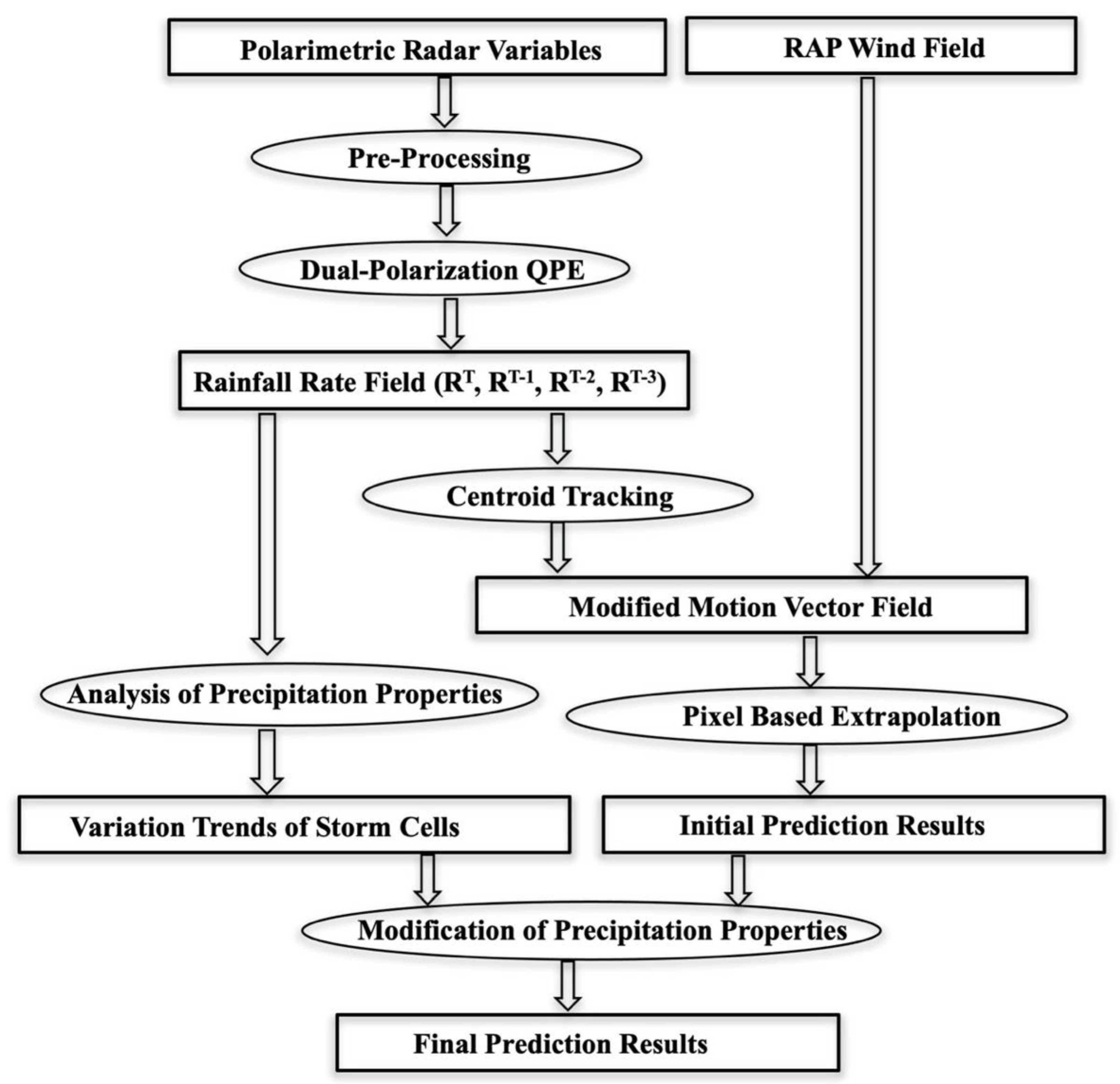
According to the QPF categories introduced in Section 1, the proposed work belongs to the extrapolation-based prediction approach, and the prediction results are calculated by linearly extrapolating the current precipitation field into the future based on the motion field. The procedures of motion field derivation and precipitation prediction are demonstrated in Figure 1. As shown in the block diagram, polarimetric radar variables and the RAP model field are used as inputs. The motion field is derived from the combination of centroid-tracking results, and the interpolated model field and the initial prediction results are calculated using the obtained motion field. The rainfall rate field derived from polarimetric radar variables is also used in the precipitation properties analysis, which is further used on adjusting the linearly extrapolated precipitation field. The processing details of the proposed approach are introduced in the following sections.

2.1. The Derived Motion Field of Radar Observations (RADAR)

2.1.1. Radar Data Processing

Different from several existing nowcasting approaches that apply a radar reflectivity field (Z) in the prediction, the proposed method utilizes a mosaicked rainfall rate (R) field instead. The advantages of applying R in the prediction are mainly from two aspects. First, in conventional approaches using single-polarization radar, Z is the only available radar variable, and R is derived through R–Z relations. Therefore, there is no significant difference between using either Z or R in the predictions. With recent developments in the polarimetric radar, a quantitative precipitation estimation (QPE) using polarimetric radar variables exhibited its advantages in accuracy and robustness. Using R can better predict a storm’s location and intensity. Another profit of the R extrapolation is that the parameters used in storm segment pairing can also be directly derived from the rainfall rate field, such as storm size and total water content. Details about these parameters will be introduced in Section 2.1.2.

In order to obtain an accurate rainfall rate field, the polarimetric radar variables of Z, differential reflectivity (Z_DR), correlation coefficient (ρ_HV), and differential phase (ϕ_DP) are processed through the following three major steps. The radar variables are first quality-controlled with a physically-based approach by Tang et al. [21] to eliminate the interference from clutters and other non-precipitation radar echoes. In this method, radar echoes from precipitation and non-precipitation are identified by a set of ρ_HV thresholds derived based on microphysics properties, including drop-size distribution, melting layer, and precipitation temperature. Pure precipitation is quality-controlled by removing interference from non-precipitation radar echoes such as biological scatter and anomalous propagation.

The quality-controlled Z and Z_DR fields are then corrected from attenuation. Different attenuation correction methods have been proposed using ϕ_DP during the past three decades, such as the linear ϕ_DP method, the standard ZPHI method, and the iterative ZPHI method [22,23,24,25]. Due to its simplicity and easy implementation in a real-time system, the linear ϕ_DP method was applied.

$$Z^c\left(r\right)=Z^o\left(r\right)+\alpha \left({\varphi }_{DP}\left(r\right)-{\varphi }_{DP}\left(0\right)\right)$$

(1)

$$Z_{DR}^c\left(r\right)=Z_{DR}^o\left(r\right)+\beta \left({\varphi }_{DP}\left(r\right)-{\varphi }_{DP}\left(0\right)\right)$$

(2)

where $Z^o\left(r\right)$ ($Z_{DR}^o\left(r\right)$ and $Z^c\left(r\right)$ ($Z_{DR}^c\left(r\right)$) are the observed (corrected) reflectivity and differential reflectivity at range r, ${\varphi }_{DP}\left(0\right)$ is the minimum system differential phase, and ${\varphi }_{DP}\left(r\right)$ is the smoothed differential phase at range r. The attenuation correction coefficients α and β depend on drop-size distribution, the drop-size-shape relation (DSR), and temperature. The typical values of α (β) are 0.01–0.04 dB/degree (0.001–0.004 dB/degree), respectively [22]. The ${\varphi }_{DP}$ is also used to estimate the specific differential phase (K_DP) through a least-square linear fitting approach.

The processed radar data (Z, Z_DR, and K_DP) are then used to estimate the rainfall rate R (mm hr⁻¹) with a synthetic method [26]. In this approach, a set of $R\left(K_{DP}\right)$, $R\left(Z, Z_{DR}\right)$, and $R\left(Z\right)$ relations are selected according to hydrometeor types. Compared with conventional R(Z) approaches, this method can produce more accurate rainfall estimation, especially for the mixture of heavy rain and hail. It should be noted that a mix of rain and hail is often observed in convective type precipitation, which is one of the focuses of QPF. An example of the reflectivity before pre-processing (A), after pre-processing (B), and an estimated rainfall rate (C) is shown in Figure 2, where the quality control process removed the non-precipitation echoes.

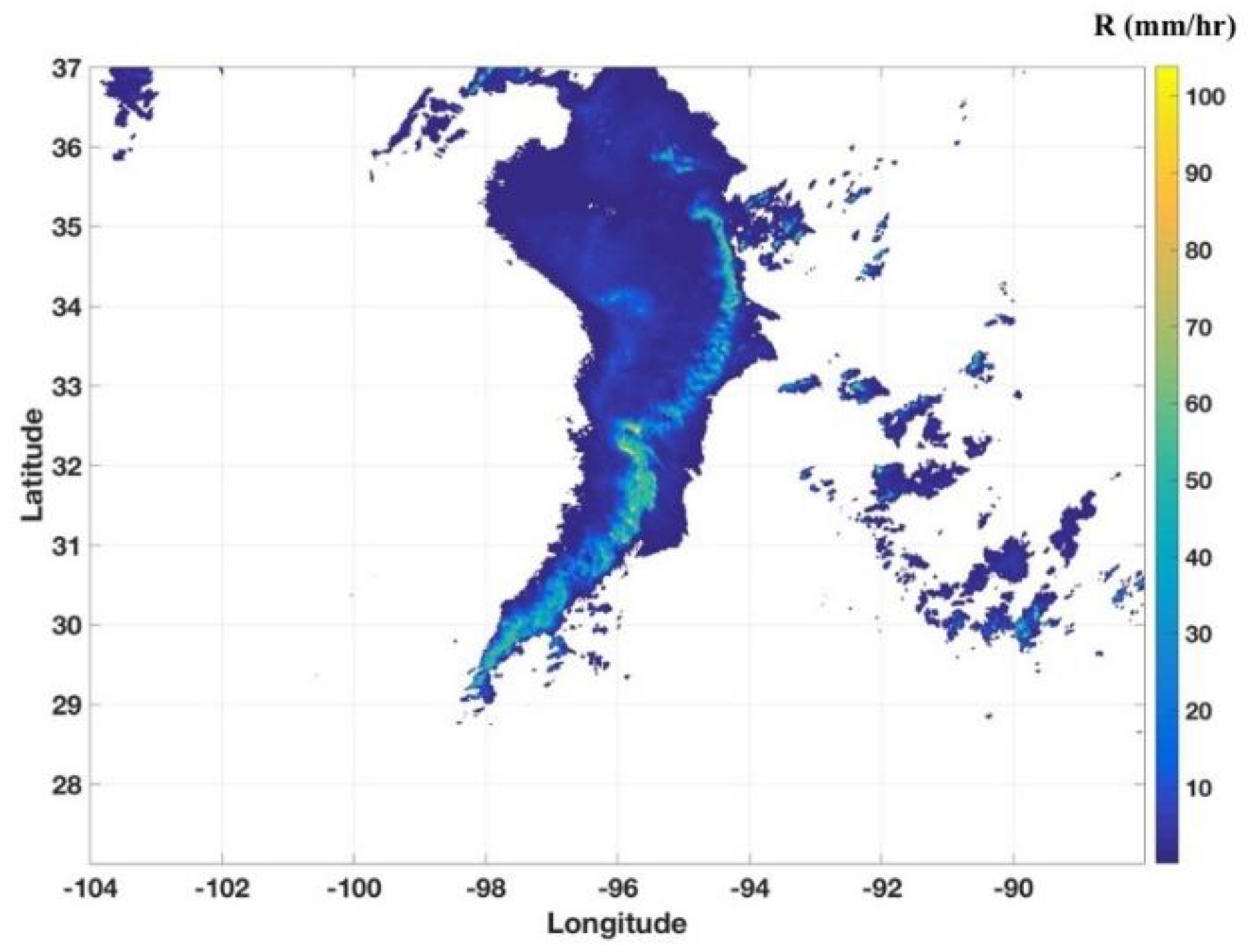
As the last step in the radar data process, the obtained rainfall rate fields from individual radars are mosaicked into a seamless precipitation field using the approach proposed by Zhang et al. [27]. An example of the mosaicked rainfall rate field is shown in Figure 3. In this example, the rainfall rate is mosaicked from 17 radars in Texas and Oklahoma, covering 25~40° N in latitude and 110~90° W in longitude. The mosaicked field rainfall rate has a spatial resolution of 1 × 1 km and a temporal resolution of 10 min.

2.1.2. Motion Field from Centroid Tracking

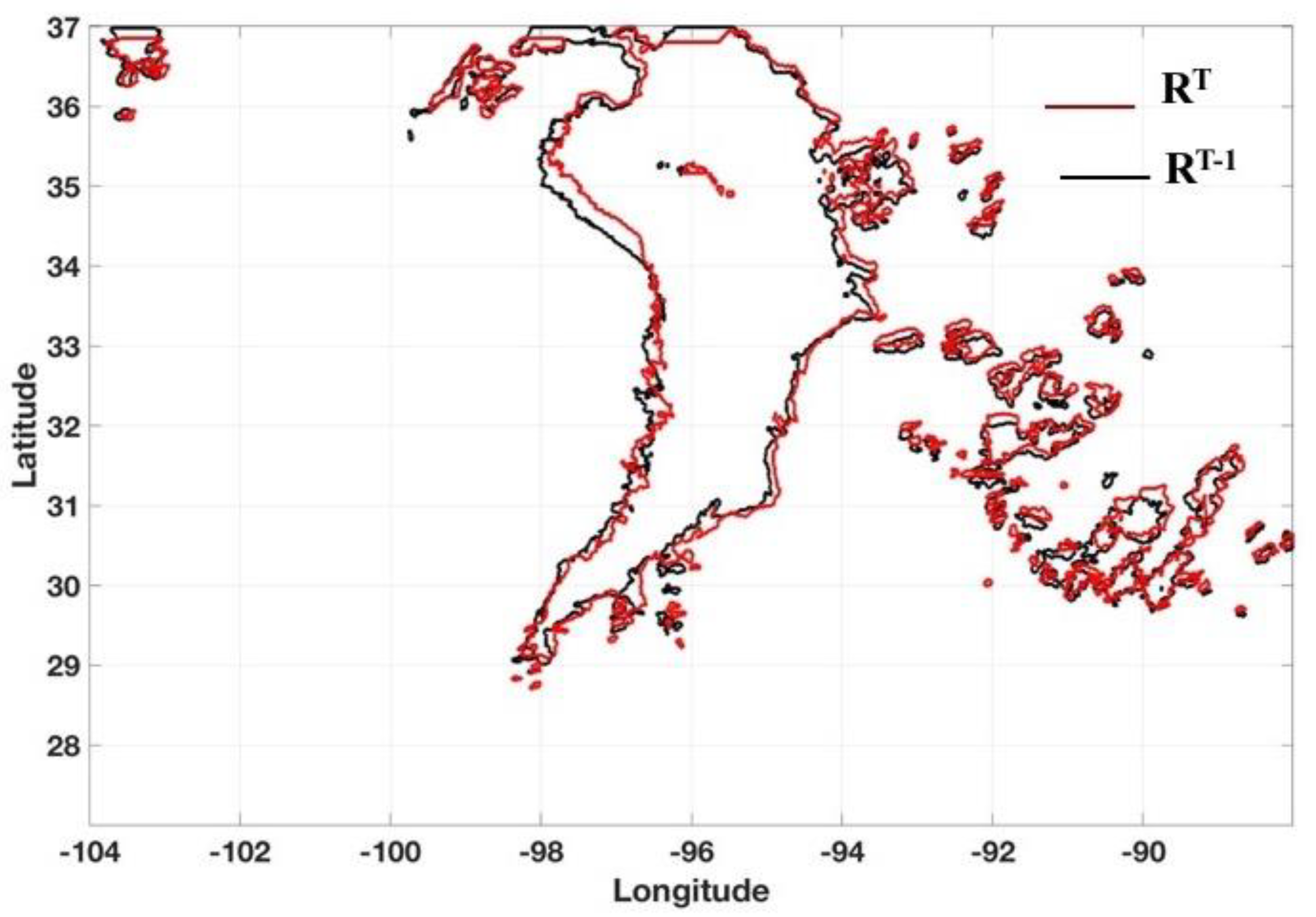
The radar-based motion field is derived using the mosaicked R fields from two continuous moments, T and T − 1. The time interval between these two adjacent moments is 10 min. An approach similar to TITAN [12,28] is applied. In this approach, the mosaicked R field is first divided into storm segments with a threshold of 0 mm hr⁻¹. An example of the segments is shown in Figure 4, where red and black lines are used to indicate the R contours (>0 mm hr⁻¹) at the current (T) moment and 10 min earlier (T − 1), respectively. In this example, a vast storm region and multiple small segments can be found in the center and eastern sides of the area, respectively. The large precipitation segment is classified as the stratiform precipitation type, which is generally associated with low rainfall rates and slow movement. The small and isolated precipitation segments located on the eastern side are classified as the convective type, generally associated with intense convection, a high rainfall rate, and fast movements.

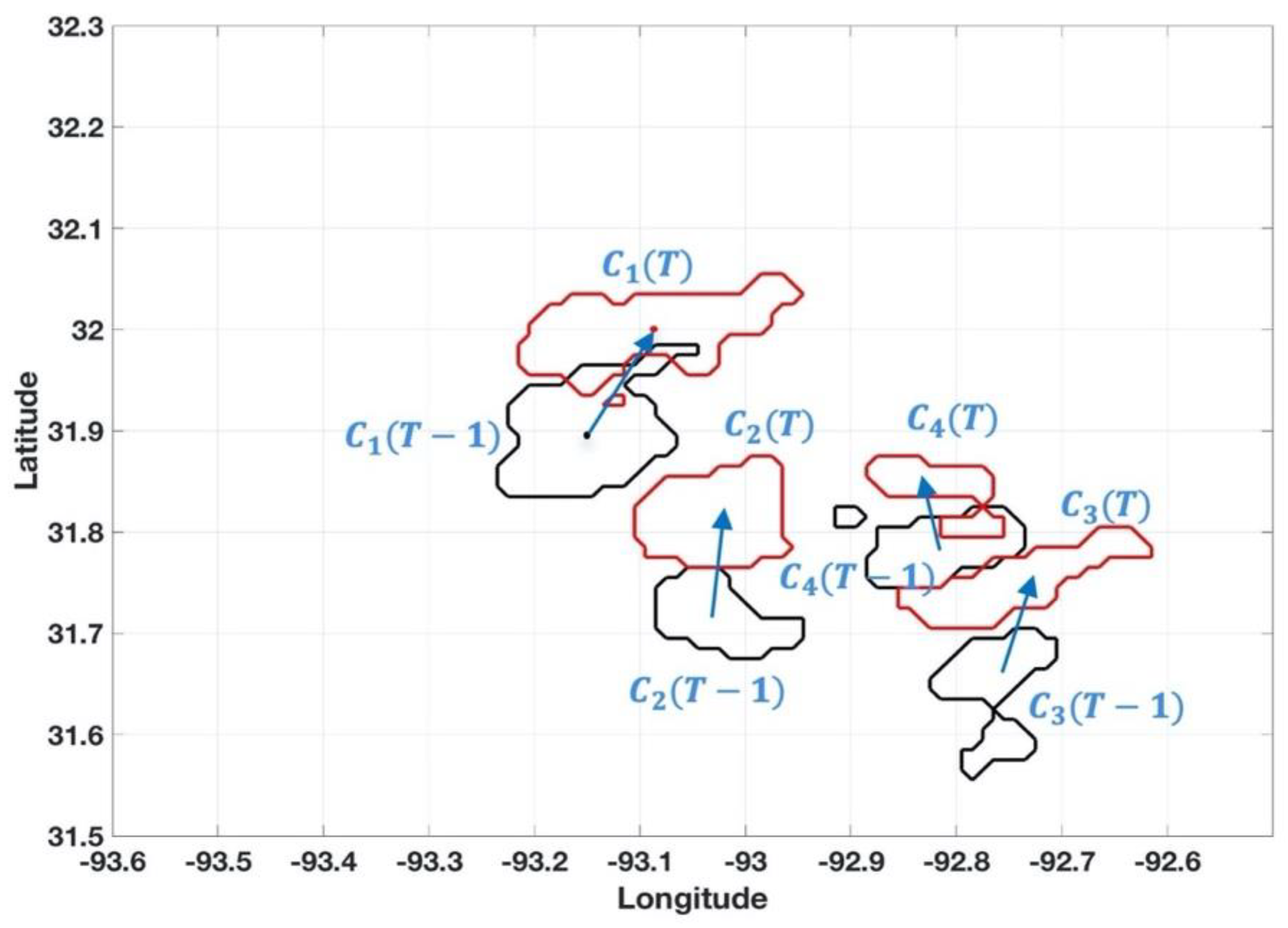
The centroid of each segment is then calculated with a K-mean method [29,30]. An enlarged area including four precipitation segments is shown in Figure 5, where red and blue colors are used to indicate cells/segments from T and $T-1$, respectively. The displacement of each segment is determined through a matching process. Within a maximum travel distance, the matching pairs (e.g., C₁($T-1$) and C₁($T$)) from the moment $T-1$ and T are associates with a short distance; similar characteristics are found in the storm size and water content (Dixon and Wiener 1993). For example, if there are total $n_1$ and $n_2$ cells identified from $T-1$ and T, there are $n_2$ possible counterparts at T for the $i^{th}$ cell (center at ($x_i^{T-1}$, $y_i^{T-1}$)) at $T-1$.

Three variables are used in the pair matching process: distance (d), total pixel (p), and summation of rainfall rate (S):

$$d_{i,j}={\left[{\left(x_i^{T-1}-x_j^T\right)}^2+{\left(y_i^{T-1}-y_j^T\right)}^2\right]}^{1/2}$$

(3)

$$p_{i,j}={\left[{\left({{\displaystyle \sum }}^{ }{p}_i^{T-1}-{{\displaystyle \sum }}^{ }{p}_j^T\right)}^2\right]}^{1/2}$$

(4)

$$S_{i,j}={\left[{\left({{\displaystyle \sum }}^{ }{R}_i^{T-1}-{{\displaystyle \sum }}^{ }{R}_j^T\right)}^2\right]}^{1/2}$$

(5)

where i and j are the cell centers from T − 1 and T, and (x,y) is the cell center. The total pixel p is used to represent the storm size, and the summation of rainfall rate S is used to represent the total water content. Unlike [12], which found the matching pairs by solving the cost function using the Hungarian method, the matched pair is identified by minimizing the normalized summation of these three factors in this work:

$$C_{i,j}=\frac{d_{i,j}}{\max \left(d\right)}+\frac{p_{i,j}}{\max \left(p\right)}+\frac{S_{i,j}}{\max \left(S\right)}.$$

(6)

The maximum travel distance is set as 20 km given the 10 min interval between T − 1 and T.

After the centroids of the paired segments from T ($C_i\left(T\right)$) and T − 1 ($C_j\left(T-1\right)$) are finalized, the motion vector is calculated using the displacement of the centroids as:

$$U^{RADAR}\left(T\right)=\frac{C_i^U\left(T\right)-C_j^U\left(T-1\right)}{\Delta T}$$

(7)

$$V^{RADAR}\left(T\right)=\frac{C_i^V\left(T\right)-C_j^V\left(T-1\right)}{\Delta T}$$

(8)

where $C^U$ and $C^V$ are the projections of the centroid coordinate onto the longitude and latitude directions. The velocity components along longitude (U) and latitude (V) are calculated using Equation (4), where $\Delta T$ is the time interval between T − 1 and T. The motion vectors using the segment results from the four segments in Figure 4 are shown in Figure 5.

2.2. Motion Field from the RAP Model

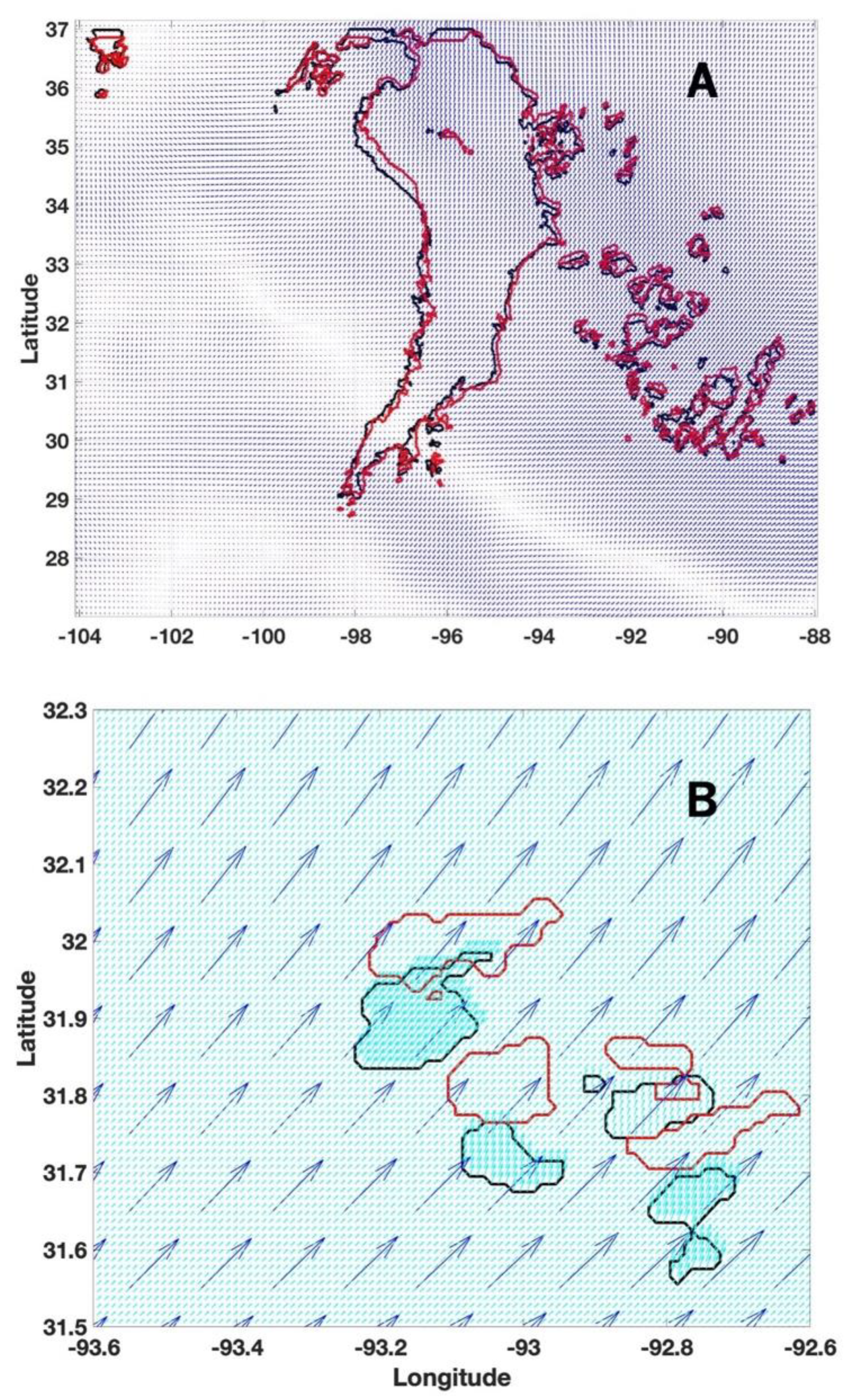
The wind field from the RAP model, an hourly updated assimilation and model forecast system, is used as another input to this algorithm. The RAP model produces horizontal wind components along longitude (U) and latitude (V) directions with a spatial resolution of 10 km by 10 km and a temporal resolution of 1 h. The RAP was implemented as an operational forecast system at the NOAA/National Centers for Environmental Prediction (NCEP) in 2012 [31]. Two layers of data are available at 700 hPa and 850 hPa reference levels. Figure 6A shows an example of the RAP model wind field from an 850 hPa layer at 2200 UTC on 25 May 2015, where the spatial resolution is 10 by 10 km.

As the radar-based motion field has a finer resolution of 1 by 1 km, the RAP model wind field is first interpolated into the same spatial resolution. Figure 6B demonstrates the original (10 by 10 km) and the interpolated (1 by 1 km) RAP wind field in the same area as Figure 5, where the same four cells are also included as references. It could be found that both the direction and magnitude of the wind field (U and V) calculated from the centroid-tracking and the model are different for all of these four cells.

2.3. Combination of Tracking and Model Wind Field

In centroid-tracking approaches such as TITAN [12], one velocity (e.g., U and V) is assigned to one segment, and all pixels within this segment are assumed to move with the same velocity. For small area segments, the single velocity may represent the whole segment movement. However, for a large area segment such as the center blob in Figure 4, a single velocity vector is not enough to capture all of the variations of the pixels. On the other hand, the RAP model provides a high-resolution velocity field capturing the pixel movements inside a large segment. However, its hourly temporal resolution significantly limits its applications in nowcasting, especially in a fast-developed convective thunderstorm. Combining the radar-based motion field and RAP model can fully utilize the advantages from these two approaches, and the prediction results are expected to be improved.

Due to the difference in temporal resolution, every set of hourly RAP data corresponds with six sets of 10 min RADAR fields. The velocity fields from the RADAR and RAP are combined through the following process. In the first step, the model velocity field ($U^{RAP}\left(T\right)$ and $V^{RAP}\left(T\right)$) at the moment T is combined with radar velocity field ($U^{RADAR}\left(t\right)$ and $V^{RADAR}\left(t\right)$) from the moments t = T, T − 1, T − 2, T − 3, T − 4, and T − 5.

$$U_{i,j}\left(t\right)=W^1\left(t\right)U_{i,j}^{RAP}\left(T\right)+W^2\left(t\right)\left(<U_{i,j}^{RAP}\left(T\right)>-U_{i,j}^{RADAR}\left(t\right)\right)$$

(9)

$$V_{i,j}\left(t\right)=W^1\left(t\right)V_{i,j}^{RAP}\left(T\right)+W^2\left(t\right)\left(<V_{i,j}^{RAP}\left(T\right)>-V_{i,j}^{RADAR}\left(t\right)\right)$$

(10)

where subscripts “$i$” and “$j$” indicate the pixel location indexes along the latitude and longitude, “< >” is the mean value of all pixels within the segment, and $W^1$ and $W^2$ are the merge coefficients. As the motion fields from the RAP model are updated every hour, its representation for the storm movement decays with the time shift. Therefore, $W^1\left(t\right)$ linearly decreases from 0.5 to 0.1 when t changes from T to T − 5 and $W^2\left(t\right)=1-W^1\left(t\right)$. In the second step, the $U_{i,j}\left(t\right)$ and $V_{i,j}\left(t\right)$ from t = T − 5 to T are averaged. The smoothed and steady averaged motion field is then used in the prediction.

2.4. Precipitation Properties and Prediction

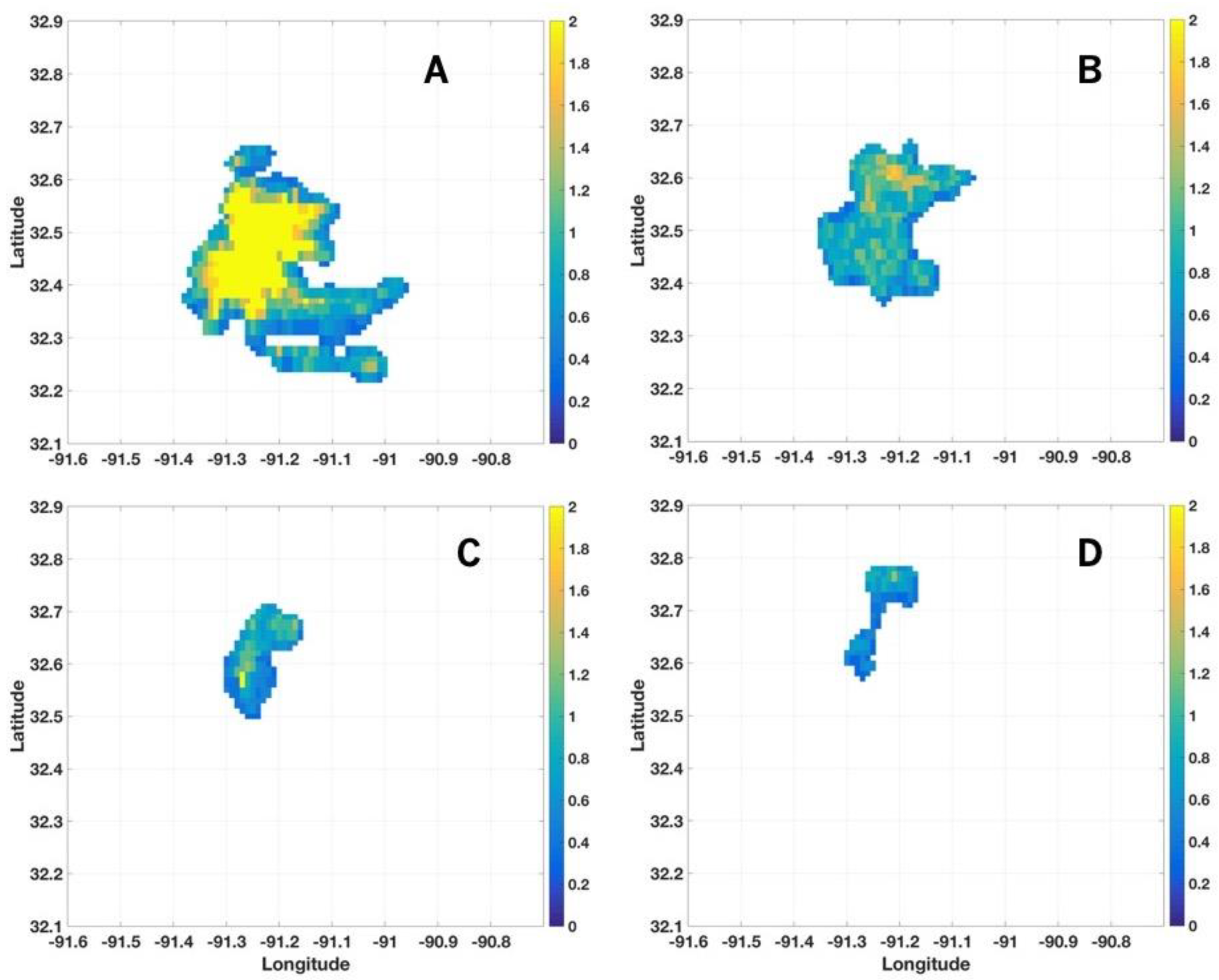
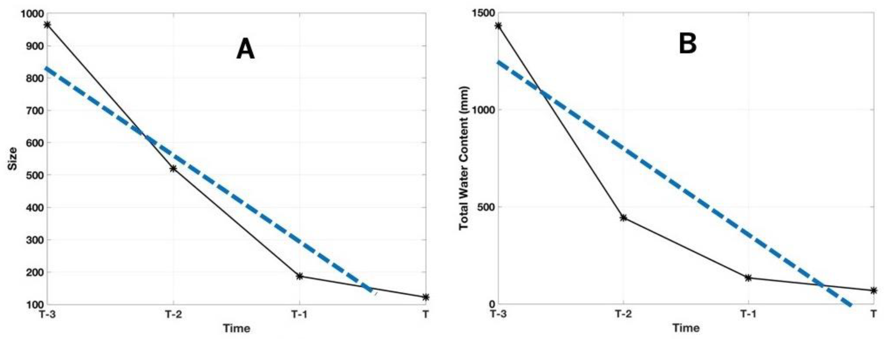
The variations of one cell from time T − 3 to T are shown in Figure 7. It can be found that not only the cell’s size shrinks from T − 3 to T, but also the total water content continuously decreases, and high-intensity (high rainfall rate) pixels disappear within the half-hour window. In order to obtain accurate results, the variations of each cell along the time need to be taken into account in the prediction. As introduced in Section 2.1.2, two variables of total pixel (p) and summation of rainfall rate (S) are used in the matching of cell pairs, and they can be viewed as the storm size and the total water content. These two variables are also used in the analysis and correction of the precipitation properties. Figure 8 shows the trends of the storm size (Figure 8A) and the total water content (Figure 8B) from T − 3 to T. The variation trends are linearly fitted, and the fitted results are further used in the prediction.

In the prediction, after the precipitation motion field is obtained through the combination of centroid-tracking and the model wind field as shown in Section 2.3, the initial prediction result is calculated through the pixel-based linear extrapolation as proposed in [12]. Specifically, each pixel will linearly move following the derived motion field. Their precipitation properties are also linearly adjusted following the linear relations shown in Figure 8. Cells merging, splitting, and dissipating are handled through the extrapolation process. For example, if two or more cells move to the same location, they will be merged, and the precipitation amounts are added together. On the other hand, if the motion field inside a large-sized cell is not uniform, this big cell may split into small pieces. The dissipating of a cell may also happen. As shown in Figure 8, if one cell shows a shrinking trend, its size and total precipitation amount will decrease in the prediction. Given enough time, the whole cell may dissipate. The emergence of new cells is beyond the extrapolation capability, therefore, not considered in the current work. In order to predict the emerging cells, a physical-based prediction model is needed and will be investigated in future work.

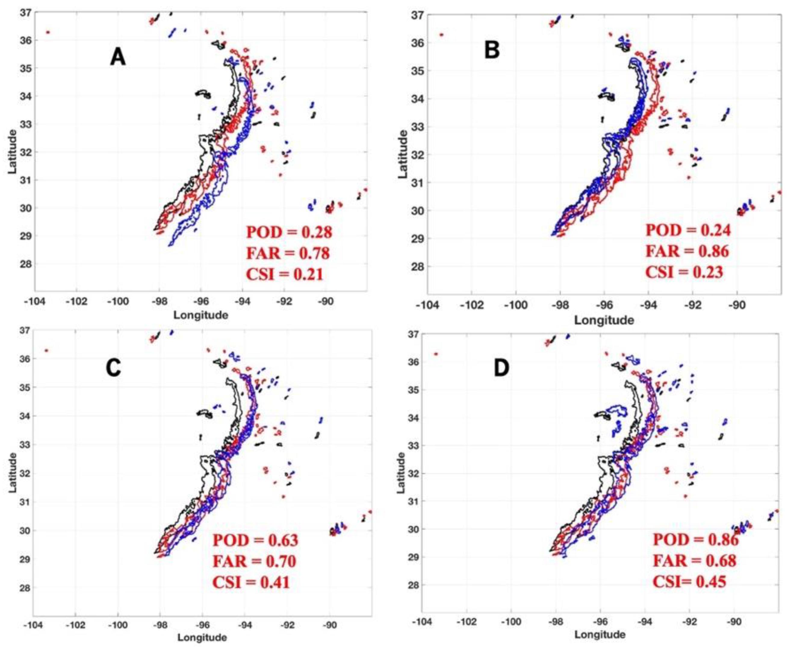
Figure 9 shows the prediction result from a thunderstorm outbreak in Oklahoma-Texas on 25 May 2015, where the domain coverage is the same as Figure 3. The mosaicked rainfall rate at 2200 UTC and 2300 UTC are shown in panels A, B. Figure 9C is the predicted rainfall rate using the proposed approach at 2300 UTC. In this example, the rainfall rate field at 2300 UTC (Figure 9B) is used as the “ground truth” to compare the prediction results. The performances from the four steps are quantitatively evaluated to demonstrate their gradual improvements. These four steps are: (I) using the motion field derived from the centroid-tracking approach only; (II) using the motion field from the model field only; (III) using the motion field combining the centroid-tracking and model field but without the adjustment of the precipitation properties and (IV) same as III but with the adjustment of the precipitation properties. Three scores of the probability of detection (POD), false alarm rate (FAR) and critical success index (CSI) are used to evaluate the performance [32]: (1) POD = a/(a + c), (2) FAR = b/(a + b), (3) CSI = a/(a + b + c) where a, b and c represent “hit”, “false” and “miss”, respectively. For any given pixel, the term “hit” is defined as both a prediction and ground truth above 10 mm/hr, “false” is the scenario when the prediction is above 10 mm/hr, but the ground truth is not, and “miss” is defined oppositely. The QPE at 2300 UTC is defined as the “ground truth”.

The evaluation results and scores of steps I–IV are presented in Figure 10A–D, respectively, where the contours are rainfall rate of 10 mm hr⁻¹ and the pixels inside the contours are associated with a rainfall rate above 10 mm hr⁻¹. The black, red, and blue lines are used to indicate the contours from the QPE at 2200 UTC, the QPE at 2300 UTC, and the prediction at 2300 UTC, respectively. It could be found that using tracking (I) or the model field only (II) cannot fully capture the movement of the storm cells and the prediction scores are low. The centroid-tracking approach can capture in real-time the overall movement. However, each cell’s movements, especially those associated with a high rainfall rate, cannot be identified. That is the primary reason for a low POD/CSI and high FAR. On the other hand, using the model field only can capture further details of the motion field. However, the low temporal resolution significantly limits its performance. The last two steps (III and IV) combine the advantages of the finer temporal resolution observed from the radar measurements and better spatial information obtained from the model field. The derived motion field can better capture the accurate storm movements and significantly enhances the prediction accuracy. Moreover, as the adjustments of the precipitation properties are included in step IV, the variations in the storm’s size and total water content are included in the prediction, and the performance is further enhanced.

3. Performance Evaluation

The performance of the proposed approach (denoted as “Proposed”) was evaluated using two hurricane precipitation events in 2017: Harvey and Irma. The prediction results from the other two approaches, using the motion field derived from the centroid-tracking method only (denoted as “Centroid-Tracking”) and using the model field only (denoted as “Model”), are also included in the evaluation for comparison purposes. The hourly prediction results were compared with the observation results. As introduced in the previous section, three scores of POD, FAR, and CSI were used in the validation where the QPE results were the ground truth.

3.1. Hurricane Harvey

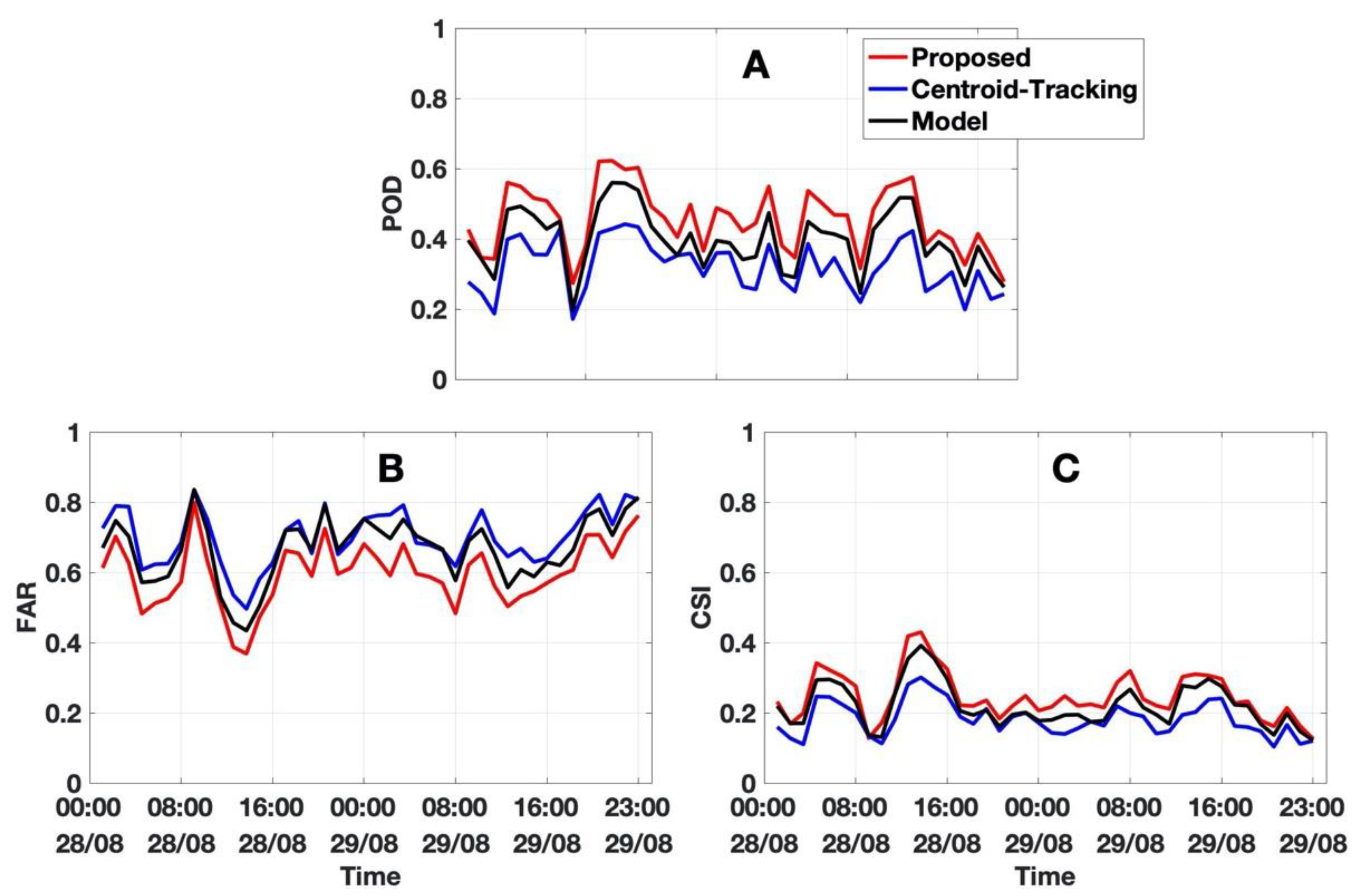
Hurricane Harvey brought significant precipitation to Texas in August 2017, causing catastrophic flooding and more than 100 deaths. It was considered the most powerful tropical cyclone rainfall event in the United States regarding its scope and peak rainfall amounts. In the current work, the performances of these three approaches were evaluated using 48 h of mosaicked radar data (28–29 August 2017). The obtained POD (A), FAR (B), and CSI (C) are shown in Figure 11, where the red, blue, and black lines indicate the results from the proposed, the centroid-tracking, and the model approach, respectively. During the 48 h, the proposed approach showed its superiorities to all three scores and produced a continuously higher POD, lower FAR, and higher CSI during the whole period. Compared with the model and centroid-tracking approaches, the average POD of the proposed approach improved about 16% and 44%; the average CSI improved 13% and 37%, and the average FAR decreased about 12% and 18%, respectively.

3.2. Hurricane Irma

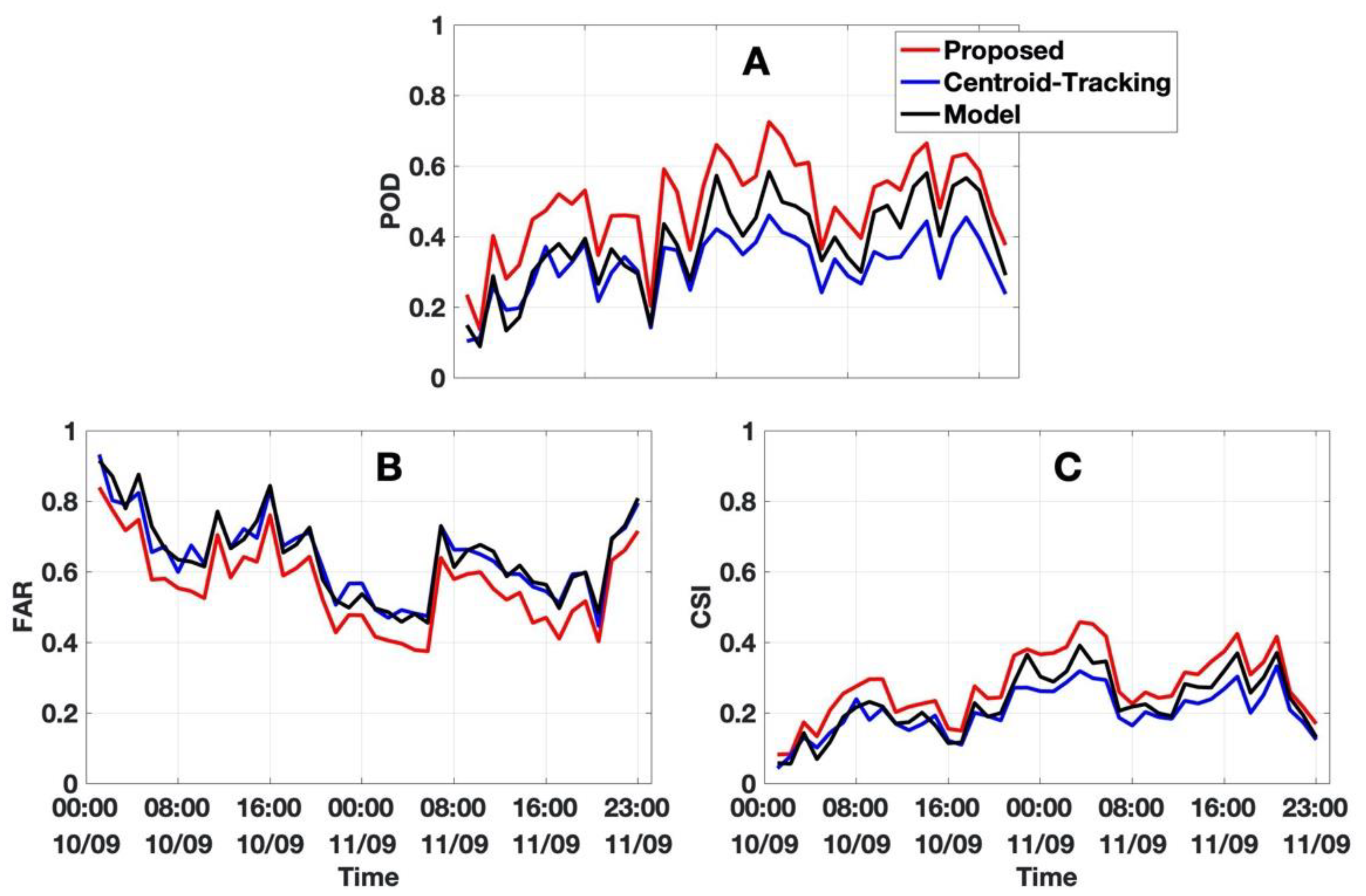
The performance of these three approaches was also validated with 48 h data from Hurricane Irma. As one of the strongest and costliest hurricanes in the Atlantic basin, Irma caused widespread destruction across its path in September 2017. A set of 48 h data (10–11 September 2017) was used in the validation, and the performance is presented in Figure 12. Similar to Harvey, the proposed approach performed better with improved scores. Compared with the model and centroid-tracking approaches, the average POD of the proposed approach improved about 33% and 55%; the average CSI improved 26% and 37%, and the average FAR decreased about 15% and 14%, respectively.

4. Summary

A novel QPF approach combining centroid-tracking and the RAP model wind field was developed and tested in the current work. The new method was unique from existing QPF approaches in two aspects. Firstly, it estimated the rainfall rate using the polarimetric data of reflectivity (Z), differential reflectivity (Z_DR), and specific differential phase (K_DP). A synthetic algorithm was used in the rainfall rate estimation, which automatically selected the optimal R(Z), R(Z, Z_DR), and R(K_DP) relations based on the precipitation types. Compared with conventional R(Z), the synthetic approach showed its advantages in robustness and accuracy. The motion field was then derived from the obtained rainfall rate field using the centroid-tracking approach. By implementing R, this method showed an advantage in improving computation efficiency as extrapolation was only acted on the R field. The direct R extrapolation could be more easily interpreted into QPE products and timely flash flood forecasts. It could also be used in the calculation of precipitation properties. Secondly, the motion field was further corrected using the RAP model field. With the corrected motion field, the prediction was generated through a linear extrapolation method. The developed approach was validated using two large-scale hurricane precipitation events. Compared with the model or centroid-tracking methods, the proposed algorithm showed a better performance with a higher POD, higher CSI, and lower FAR.

The proposed algorithm handled the merging, splitting, and dissipating of cells through an extrapolation approach. However, the emergence of new cells could not be predicted by this approach. Modifications such as an additional physical-based model could further enhance the prediction of emerging cells in the future.

References

- Wilson, J.; Crook, N.A.; Mueller, C.K.; Sun, J.; Dixon, M. Nowcasting thunderstorms: A status report. Bull. Amer. Meteor. Soc. 1998, 79, 2079–2099. [Google Scholar] [CrossRef]
- Wilson, J. Thunderstorm nowcasting: Past, present and future. In Proceedings of the 31st Conference on Radar Meteorology, American Meteorological Society, Seattle, WA, USA, 7–12 August 2003. [Google Scholar]
- Rinehart, R.E.; Garvey, E.T. Three-dimensional storm motion detection by conventional weather radar. Nature 1978, 273, 287–289. [Google Scholar] [CrossRef]
- Rinehart, R.E. A pattern recognition technique for use with conventional weather radar to determine internal storm motions. Atmos. Technol. 1981, 13, 119–134. [Google Scholar]
- Bellon, A.; Austin, G.L. The accuracy of short-term rainfall forecasts. J. Hydrol. 1984, 70, 35–49. [Google Scholar] [CrossRef]
- Li, L.; Schmid, W.; Joss, J. Nowcasting of motion of precipitation with radar over complex terrain. J. Appl. Meteor. 1995, 34, 1286–1298. [Google Scholar] [CrossRef] [Green Version]
- Ryall, G.; Conway, B.W. Automated precipitation nowcasting at the UK Met Office. In First European Conf. on Applications of Meteorology; University of Oxford: Oxford, UK, 1994. [Google Scholar]
- Pierce, C.E.; Ebert, E.; Seed, A.W.; Sleigh, M.; Collier, C.G.; Fox, N.I.; Donaldson, N.; Wilson, J.W.; Roberts, R.; Mueller, C.K. The nowcasting of precipitation during Sydney 2000: An appraisal of the QPF algorithm. Weather Forecast. 2004, 21, 7–21. [Google Scholar] [CrossRef]
- Austin, G.L.; Bellon, A. Very-short-range forecasting of precipitation by the objective extrapolation of radar and satellite data; Browning, K.A., Ed.; Nowcasting Academic Press: London, UK, 1982; pp. 177–190. [Google Scholar]
- Rosenfeld, D. Objective method for analysis and tracking of convective cells as seen by radar. J. Atmos. Ocean. Technol. 1987, 4, 422–434. [Google Scholar] [CrossRef] [Green Version]
- Tuttle, J.D.; Foote, G.B. Determination of the boundary layer airflow from a single Doppler radar. J. Atmos. Ocean. Technol. 1989, 7, 218–232. [Google Scholar] [CrossRef] [Green Version]
- Dixon, M.; Weiner, G. TITAN: Thunderstorm Identification, Tracking Analysis and Nowcasting—A radar-based methodology. J. Atmos. Ocean. Technol. 1993, 10, 785–797. [Google Scholar] [CrossRef]
- Johnson, J.T.; Mackeen, P.L.; Witt, A.; Mitchell, D.; Stumpf, G.J.; Eilts, M.D.; Thomas, K.W. The storm cell identification and tracking algorithm: An enhanced WSR-88D algorithm. Weather Forecast. 1998, 13, 263–276. [Google Scholar] [CrossRef] [Green Version]
- Lakshmanan, V.; Smith, T. An objective method of evaluating and devising storm-tracking algorithms. Weather Forecast. 2010, 25, 701–709. [Google Scholar] [CrossRef]
- Bowler, N.E.; Pierce, C.E.; Seed, A.W. SETPS: A probabilistic precipitation forecasting scheme which merges an extrapolation nowcast with downscaled NWP. Quart. J. Roy. Meteor. Soc. 2006, 132, 2127–2155. [Google Scholar] [CrossRef]
- Bellon, A.; Zawadzki, I.; Kilambi, A.; Lee, H.C.; Lee, Y.H.; Lee, G. McGill algorithm for precipitation nowcasting by Lagrangian extrapolation (MAPLE) applied to the South Korean radar network. Part I: Sensitivity studies of the Variational Echo Tracking (VET) technique. Asia Pac. J. Atmos. Sci. 2010, 46, 369–381. [Google Scholar] [CrossRef]
- Atencia, A.; Zawadzki, I. A comparison of two techniques for generating nowcasting ensembles. Part I: Lagrangian ensemble technique. Mon. Wea. Rev. 2014, 142, 4036–4052. [Google Scholar] [CrossRef]
- Germann, U.; Zawadzki, I. Scale dependence of the predictability of precipitation from continental radar images. Part II: Probability forecasts. J. Appl. Meteor. 2004, 43, 74–89. [Google Scholar] [CrossRef]
- Li., P.W.; Wong, W.K.; Lai, S.T. RAPIDS-A new rainstorm nowcasting system in Hong Kong. In Proceedings of the WMO/WWRP International Symposium on Nowcasting and Very-Short-Range Forecasting, Toulouse, France, 5–9 September 2005; HongKong Observatory Toulouse. [Google Scholar]
- Seed, A.W. A dynamic and spatial scaling approach to advection forecasting. J. Appl. Meteor. 2003, 42, 381–388. [Google Scholar] [CrossRef]
- Tang, L.; Zhang, J.; Langston, C.; Krause, J.; Howard, K.; Lakshmanan, V. A physically based precipitation-nonprecipitation radar echo classifier using polarimetric and environmental data in a real-time national system. Weather Forecast. 2014, 29, 1106–1118. [Google Scholar] [CrossRef]
- Jameson, A.R. The effect of temperature on attenuation correction schemes in rain using polarization propagation differential phase shift. J. Appl. Meteor. 1992, 31, 1106–1118. [Google Scholar] [CrossRef] [Green Version]
- Carey, L.D.; Rutledge, S.A.; Ahijevych, D.A.; Keenan, T.D. Correcting propagation effects in C-band polarimetric radar observations of tropical convection using differential propagation phase. J. Appl. Meteor. 2000, 39, 1405–1433. [Google Scholar] [CrossRef] [Green Version]
- Testud, J.E.; Bouar, L.; Obligis, E.; Ali-Mehenni, M. The rain profiling algorithm applied to polarimetric weather radar. J. Atmos. Ocean. Technol. 2000, 17, 322–356. [Google Scholar] [CrossRef]
- Park, S.G.; Maki, M.; Iwanami, K.; Bringi, V.N.; Chandrasekar, V. Correction of radar reflectivity and differential reflectivity for rain attenuation at X-band. Part II: Evaluation and application. J. Atmos. Ocean. Technol. 2005, 22, 1633–1655. [Google Scholar] [CrossRef]
- Giangrande, S.; Ryzhkov, A. Estimation of rainfall based on the results of polarimetric echo classification. J. Appl. Meteor. 2008, 47, 2445–2462. [Google Scholar] [CrossRef]
- Zhang, J.; Howard, K.; Langston, C.; Kaney, B.; Qi, Y.; Tang, L.; Grams, H.; Wang, Y.; Cocks, S.; Martinaitis, S.; et al. Multi-radar multi-sensor (MRMS) quantitative precipitation estimation: Initial operating capabilities. Bull. Amer. Meteor. Soc. 2016, 97, 621–638. [Google Scholar] [CrossRef]
- Han, L.; Fu, S.; Zhao, L.; Zhang, Y.; Wang, H.; Lin, Y. 3D convective storm identification, tracking, and forecasting—an enhanced TITAN algorithm. J. Atmos. Ocean. Technol. 2008, 26, 719–732. [Google Scholar] [CrossRef]
- Spath, H. Cluster Dissection and Analysis: Theory, FORTRAN Programs, Examples; Goldschmidt, J., Translator, Eds.; Halsted Press: New York, NY, USA, 1985. [Google Scholar]
- Arthur, D.; Vassilvitskii, S. K-means++: The Advantages of Careful Seeding. In Proceedings of the Eighteenth Annual ACM-SIAM Symposium on Discrete Algorithms, New Orleans, LA, USA, 7–9 January 2007; pp. 1027–1035. [Google Scholar]
- Stanley, G.B.; Weygandt, S.S.; Brown, J.M.; Hu, M.; Alexander, C.R.; Smirnova, T.G.; Olson, J.B.; James, E.P.; Dowell, D.C.; Grell, G.A.; et al. A north American hourly assimilation and model forecast cycle: The rapid refresh. Mon. Wea. Rev. 2016, 144, 1669–1694. [Google Scholar]
- Mitchell, E.D.; Vasiloff, S.V.; Stumpf, G.J.; Witt, A.; Eilts, M.D.; Johnson, J.T.; Thomas, K.W. The National Severe Storm Laboratory tornado detection algorithm. Weather Forecast. 1998, 13, 352–366. [Google Scholar] [CrossRef]
Figure 1.
The flow chart of the proposed radar-based QPF approach.
Figure 2.
The reflectivity fields from (A) before and (B) after the quality control process and (C) the estimated rainfall rate using polarimetric radar variables.
Figure 3.
The rainfall rate mosaic at 2210 UTC 25 May 2015.
Figure 4.
The contours of the rainfall rate (R) fields. The segmentations of R at 2210 UTC (RT) and 10 min prior () are represented by red and black lines, respectively.
Figure 5.
Motion vectors from four cells (C1, C2, C3, and C4).
Figure 6.
(A) The model wind field in the domain with a latitude of 27° to 37° and a longitude of −104° to −88°. (B) The model wind field in a zoomed-in region centered at (31.9°, −93.1°). The original (10 km by 10 km) and interpolated (1 km by 1 km) wind fields are shown with blue and cyan color, respectively. The model data are from 2200 UTC, 25 May 2015.
Figure 7.
Example of one precipitation segment at (A) , (B) , (C) , and (D) T.
Figure 8.
The trend of (A) the precipitation’s size and (B) the precipitation’s total water content. The calculated variables are presented with solid black lines, and linearly fitted results are shown with dashed blue lines.
Figure 9.
(A) QPE results at 2200 UTC; (B) QPE results at 2300 UTC; (C) prediction results at 2300 UTC.
Figure 10.
The results of (A) applying centroid-tracking only; (B) using the model field only; (C) from the combination of centroid-tracking and the model field without the adjustment of the precipitation properties; (D) similar to (C) but with the adjustment of the precipitation properties. The QPE at 2200 UTC, QPE at 2300 UTC, and prediction at 2300 UTC are indicated by black, red, and blue lines.
Figure 11.
The statistical score of (A) the probability of detection, (B) the false alarm rate, and (C) the critical success index. The red, blue, and black lines show the proposed, the centroid-tracking, and the model results. A set of 48 h of data from 28–29 August 2017 is used in the analysis.
Figure 12.
Similar to Figure 11, with 48 h of data from Hurricane Irma (10–11 September 2017).
Publisher’s Note: MDPI stays neutral with regard to jurisdictional claims in published maps and institutional affiliations. |
© 2021 by the authors. Licensee MDPI, Basel, Switzerland. This article is an open access article distributed under the terms and conditions of the Creative Commons Attribution (CC BY) license (https://creativecommons.org/licenses/by/4.0/).
Share and Cite
MDPI and ACS Style
Wang, Y.; Tang, L. A Short-Term Quantitative Precipitation Forecasting Approach Using Radar Data and a RAP Model. Geomatics 2021, 1, 310-323. https://0-doi-org.brum.beds.ac.uk/10.3390/geomatics1020017
AMA Style
Wang Y, Tang L. A Short-Term Quantitative Precipitation Forecasting Approach Using Radar Data and a RAP Model. Geomatics. 2021; 1(2):310-323. https://0-doi-org.brum.beds.ac.uk/10.3390/geomatics1020017
Chicago/Turabian StyleWang, Yadong, and Lin Tang. 2021. "A Short-Term Quantitative Precipitation Forecasting Approach Using Radar Data and a RAP Model" Geomatics 1, no. 2: 310-323. https://0-doi-org.brum.beds.ac.uk/10.3390/geomatics1020017