
Precipitation Data Retrieval and Quality Assurance from Different Data Sources for the Namoi Catchment in Australia

Hydro & Meteo GmbH, Breite Straße 6-8, 23552 Lübeck, Germany
*
Author to whom correspondence should be addressed.
Geomatics 2021, 1(4), 417-428; https://0-doi-org.brum.beds.ac.uk/10.3390/geomatics1040024
Submission received: 17 August 2021
/
Revised: 17 September 2021
/
Accepted: 20 September 2021
/
Published: 28 October 2021
(This article belongs to the Special Issue Remote Sensing for Precipitation Retrievals)
Abstract
:Within the Horizon 2020 Project WaterSENSE a modular approach was developed to provide different stakeholders with the required precipitation information. An operational high-quality rainfall grid was set up for the Namoi catchment in Australia based on rain gauge adjusted radar data. Data availability and processing considerations make it necessary to explore alternative precipitation approaches. The gauge adjusted radar data will serve as a benchmark for the alternative precipitation data. The two well established satellite-based precipitation datasets IMERG and GSMaP will be analyzed with the temporal and spatial requirements of the applications envisioned in WaterSENSE in mind. While first results appear promising, these datasets will need further refinements to meet the criteria of WaterSENSE, especially with respect to the spatial resolution. Inferring information from soil moisture-derived from EO observations to increase the spatial detail of the existing satellite-based datasets is a promising approach that will be investigated along with other alternatives.
1. Introduction
Australia is a continent where precipitation measurement information availability is very heterogeneous. This is the starting point for the WaterSENSE project, where remote sensing data are used to provide more uniform information across Australia. This project has received funding from the Horizon 2020 research and innovation programme under grant agreement No 870344. It has a duration from January 2020 to December 2023.
The goal of WaterSENSE is to develop a modular, operational, water-monitoring system built on Copernicus EO (Earth Observation) data. This will provide water managers and the agricultural sector with a toolbox of reliable and actionable information on water availability and water use, anywhere in the world, in support of sustainable water management and transparency across the entire water value chain.
To achieve this goal, we designed a testbed of carefully quality controlled radar data in the Namoi catchment. The purpose of this testbed is to serve as a benchmark for other precipitation sources that are more widely available over Australia than radar. Therefore, we adjust Namoi radar data with rain gauge data in order to generate a high-quality gridded precipitation dataset with good temporal and spatial resolution [1,2]. Due to their near-global availability, we will focus on the existing multi-instrument precipitation products IMERG [3] and GSMaP [4]. The precipitation dataset derived from radar data allows us to investigate the quality of these datasets on different temporal and spatial scales [5,6]. In order to improve the spatial resolution of this data, we are planning to investigate and refine methods based on soil moisture from EO data such as SM2Rain [7]. Soil moisture from Copernicus EO data is also derived within this project.
2. Application Driven Requirements on Precipitation Data within WaterSENSE
A critical task within WaterSENSE will be to provide more spatial and temporal detail in existing gridded rainfall data and rainfall forecast maps by integrating Copernicus EO data into existing methods, keeping in mind the requirements of different applications. This is because the location, timing, duration, and intensity of precipitation plays a central role in the functioning of water systems, both urban and rural. Accurate and timely quantitative precipitation information is vitally important for water managers to effectively plan, design, operate and maintain their water systems.
The agricultural sector relies on information on a spatial scale comparable to a plot size. This sets the demand for data with a spatial resolution of not more than 1 km². The required temporal resolution is in the order of days to one month, while a latency of several days is acceptable.
The requirements for hydrological applications are different. The spatial resolution of the data should also be approximately 1 km². The desired time resolution is hours or preferably shorter with a latency of no more than 15 min for warning applications.
Therefore, a framework has been developed for setting up multi-level precipitation information for Australia, using different data sources and data qualities. The idea is to provide a base level of precipitation data quality everywhere in Australia, and use higher-quality data wherever available. This approach has been set up for the Namoi catchment.
3. Data Verification Setup in the Namoi Catchment
3.1. Verification Strategy
Under normal conditions rain gauges measure precipitation amounts with high accuracy and varying temporal resolutions and latencies depending on the instrument type and the data flow [8]. This can range from data with a resolution of one minute which is available in real-time to data that has a resolution of one day and longer and is only available after several days. However, the main limitation of these data is their inhomogeneous availability, with typically less data in rural areas, together with its limited spatial representativeness. Additionally, rain gauges may underestimate rainfall in windy conditions [9]. Radar data, with a spatial resolution which is typically in the order of 1 km², on the other hand is well suited to capture spatial precipitation patterns. In addition, the temporal resolution of 5 to 10 min and the latency of typically less than 5 min are ideal for many applications. The accuracy of estimating precipitation amounts by radar alone is limited by variable drop size distributions among other factors. Carefully combining quality-controlled data from automatically reporting rain gauges and radar data yields a dataset with a high accuracy, a good temporal and spatial resolution, and a low latency, together with a good spatial coverage.
Therefore, we choose gauge adjusted radar data as the benchmark for other remotely sensed precipitation data. This approach was already successfully used by others such as [5,10]. However, the gauge adjusted radar data will not only be used as a benchmark, but also serve as a product in WaterSENSE where available.
The statistical properties of all remotely sensed data in the project on different spatial and temporal scales will be evaluated according to the application requirements outlined in Section 2 and compared to the results based on adjusted radar data.
3.2. Namoi Catchment
The Namoi catchment is a large catchment located in New South Wales, Australia. Its name originates from the Namoi river, which flows through the catchment from the northeast to the southwest and which is the main source of irrigated water. The catchment is shown in Figure 1 along with the radar coverage and several rain gauge stations. It is characterized as a region with intensive agriculture with extensive cotton plantations.
The precipitation regime of the Namoi catchment is spatially very inhomogeneous. The Eastern part of the catchment close to the Great Dividing Range has a relatively wet climate with a maximum average (1976–2005) annual rainfall of 1300 mm. In contrast the low-lying plains situated in the Western part of the catchment exhibit a predominantly semi-arid climate with an average annual rainfall of approximately 400 mm near Walgett. Generally, summer and winter are the wettest months, with the winter rainfall being especially relevant for dam inflows. However, also the annual rainfall amounts are highly variable with multi-decadal wet and dry periods with intermittent periods of droughts and high rainfall, respectively. Currently, the Namoi catchment is in a dry period, with 2017 to 2020 being the driest period on record. Nevertheless, the entire region is prone to flooding [11].
3.3. Namoi Weather Radar
The Namoi weather radar is operated by the Bureau of Meteorology. It is an S-band radar covering a nominal range of 300 km. Its location (lat 31.0240°, long 150.1915°) on top of Black Jack Mountain at an elevation of 699 m means that it can observe precipitation in a 360 degree window, but it also limits the range, depending on the elevation angle and the meteorological situation, until where precipitation can be observed. Additionally, the complex terrain surrounding the radar can obstruct the radar beam at low elevation angles, making it difficult to observe low-level precipitation, especially to the south and southwest of the radar. The complex topography within the radar range can cause non-meteorological echoes especially under anomalous propagation conditions.
We obtained near-real-time radar data for this project in two different formats:
- Prior to October 2020 (polar data with a radial resolution of 500 m and a temporal resolution of 10 min)
- After October 2020 (polar data with a radial resolution of 250 m and a temporal resolution of 5 min)
This is relevant not only for the importer into our radar data analysis and correction software SCOUT (Second Moments Cloud Tracking) [12], but also for the applied correction procedures because of the different spatial and temporal characteristics associated with the different datasets. All data were obtained from the Bureau of Meteorology and was already pre-processed at the radar site. The key specifications of the radar data are summarized in Table 1.
3.4. Radar Data Processing
As described above, the radar data are generally well suited to observe precipitation in the majority of the Namoi catchment. With this radar data and rain gauge data as inputs we developed a rectangular rainfall grid with a 1 km resolution. Processing of the radar data involved addressing the remaining errors in the data with the help of the radar data analysis and processing software SCOUT. The most relevant filters are:
- Clutter map: A radar-specific clutter map has been semi-automatically created based on the historical period (17 April 2020–11 October 2020). Pixels included in the clutter map are permanently deleted and replaced by an interpolation of the neighbouring pixels. Typical applications include the removal of clutter from mountains and towers.
- Speckle filter: This filter removes very small echoes (e.g., ships and air planes), defined by a configurable upper threshold for the number of non-zero pixels, which are surrounded by zero pixels. The filter can either operate on the whole image or on predefined pixels only.
- Reverse speckle filter: This filter deletes groups of zero pixels which are surrounded by non-zero pixels. The threshold for the maximum number of pixels can be configured. The filter can either operate on the whole image or on predefined pixels only.
- Gabella filter: A texture-based filter [13] is used to smooth extreme peaks in the image, e.g., due to ground clutter within a rain field. The filter can either operate on the whole image or on predefined pixels only.
- Beam blockage filter: A measurement data-based method to correct for beam blockage in polar radar data, which does not require the existence of a digital elevation model or precise knowledge about the radar parameters as other methods do [14]. Instead, a careful visual and statistical analysis of the radar data leads to the determination of beam-specific correction factors.
- Advection correction: This correction overcomes the fact that radar measurements are instantaneous measurements and do not provide rainfall volumes in time. Precipitation cells are detected and identified in consecutive images. A field of motion vectors is calculated, and the precipitation is distributed along the track of the cells based on the motion vector field. This gives a more realistic spatial distribution of the precipitation [15].
Another important step to increase the accuracy of the precipitation estimate is to adjust the radar data based on a comparison with rain gauge data [16]. Correction factors are calculated at all rain gauge locations and interpolated to the entire spatial domain. Different interpolation methods are implemented in SCOUT. Here, an interpolation method was chosen which uses a weighted mean of the correction factors at all stations for every pixel. The weight , where d is the distance from the rain gauge. This results in a relatively smooth correction factor field with moderate inhomogeneities at each station to account for the local correction factors. The adjustment can either be carried out in near real-time or as post processing depending on the user requirements. The latter methods give systematically better results because radar and rain gauge data are compared for a period which includes the time step that is being adjusted. In contrast, the time constraints of near real-time adjustment mean that a recent comparison of rain gauge and radar data is used to adjust the current time step which is not included in this recent comparison interval. One of the sources of uncertainties in the adjustment process is caused by the different spatial representativeness of the two instruments. Differences in rain gauge measurements as large as 20% have been found over an area of one square kilometer, the typical size of a radar pixel [17].
When preparing the dataset, first a radar elevation was chosen as working level. Generally, data from lower elevations are a better representation of the precipitation at the ground but can be contaminated by clutter and other artefacts. Higher elevations typically have fewer problems with clutter. However, the useful spatial range (the range up to which the measurement shows differences in the values and is comparable to ground station measurements) can be limited by overshooting, e.g., when the radar beam at a certain distance from the radar is so high above the ground that it misses part of or all the precipitation. Data from 17 April 2020 until 6 July 2020 from the lowest three elevation angles, 0.5°, 0.9° and 1.3° respectively, were analyzed. Most errors become more obvious when data is accumulated over a period. Looking at the images of Figure 2, the elevation of 0.9° was chosen because its useful spatial range is similar to that of the data at 0.5° and better than the data at 1.3°. Furthermore, the data at 0.9° are less affected by clutter, beam blockage and areas with zero precipitation embedded in precipitation fields. After the application of the clutter map, the speckle filter, the reverse speckle filter, the Gabella filter, and the beam blockage filter, no beam blockage is shown in the cumulated precipitation field except for the area south-west of the radar at large distances from the radar where data are also affected by overshooting. Additionally, the cumulated precipitation field shows less clutter and significantly reduced areas with zero or very low precipitation (Figure 2).
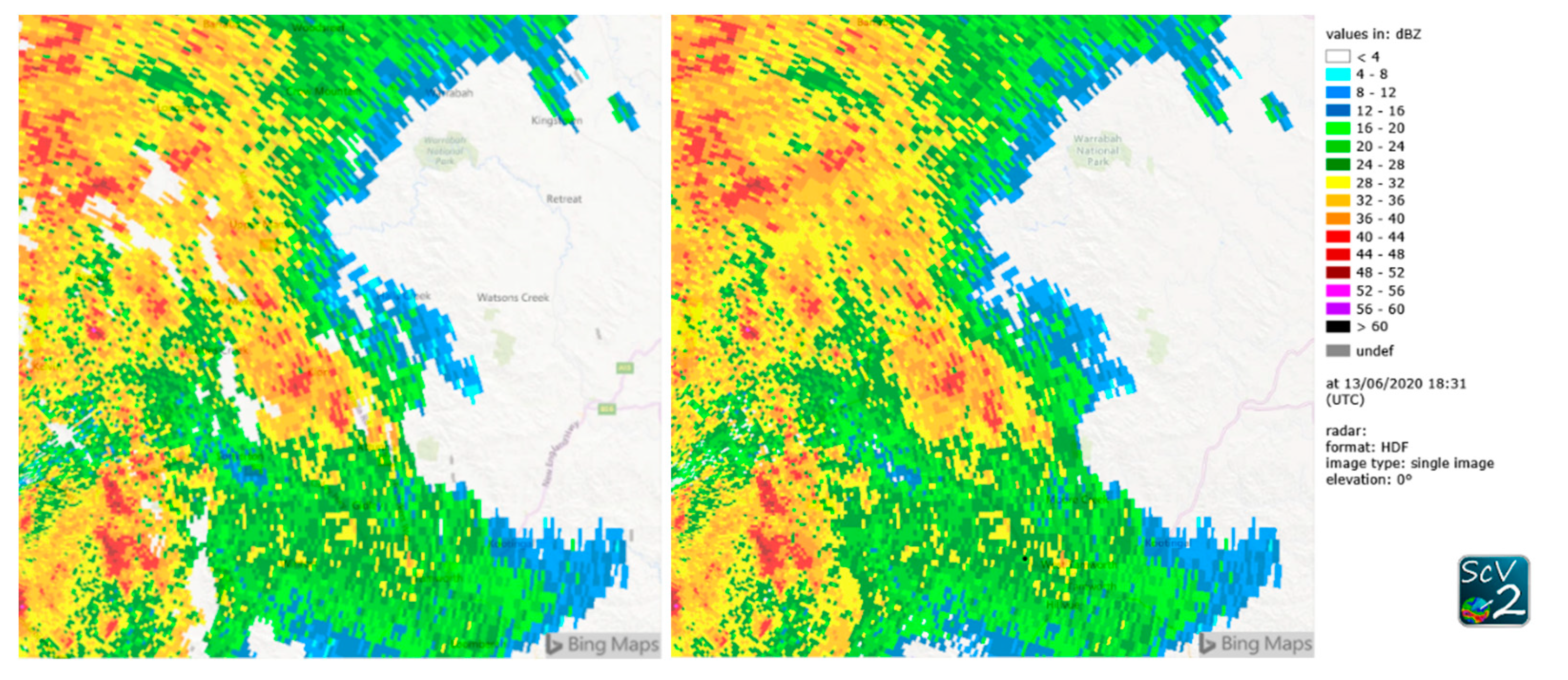
While the effect of the filters can be seen in the cumulated images of Figure 2, the filters are applied to single radar images. Therefore, the effect of the filters can also be shown for individual images. Figure 3 shows a single radar image before and after the above filters have been applied. The majority of the non-zero pixels not associated with precipitation have been removed.
Figure 4 shows an area of the image where the reverse speckle filter has been used. Here, the “holes” in the data are relatively large and consequently a large threshold for the maximum number of zero pixels had to be chosen. To limit undesired effects, the application of the filter has been restricted to predefined areas. These areas were identified from the cumulated image. After the application of the filters, the “holes” have been filled with more realistic precipitation values through spatial interpolation.
The effect of the advection filter is shown in Figure 5, where the cumulated precipitation is shown for one day. Before the corrections, areas with more and less precipitation alternate. After the advection correction, the precipitation is distributed more realistically along the tracks of the cells. It is very important to perform this correction before the adjustment with rain gauge data, because for rain gauges lying in maximum and minimum areas of the radar precipitation, wrong correction factors would otherwise be inferred.
After adjustment with station data the median of the difference between the radar data and the station data was 6%.
The station YWLG in the north-west of the catchment was unusual, since the station measured 122.4 mm in this period, while only 11.06 mm were inferred from the radar measurements. This difference is caused by overshooting, where the radar is measuring above the rain fields and cannot be corrected for. Therefore, the precipitation in the north-west of the catchment is considerably underestimated in the radar data even after correction and adjustment.
Figure 6 shows the cumulated images before and after all corrections have been performed. The image with corrections looks much smoother compared to the cumulated image before the advection correction. The radar-gauge adjustment increases the amount of the precipitation slightly in most areas while the spatial distribution of the precipitation is only altered slightly by the adjustment process. Again, the underestimation of the precipitation in the northwest of the catchment can be seen.
Transferring the above achievements and settings to the data after October 2020, some minor adjustments have been performed. Firstly, as it was apparent that the useful range of the radar data was significantly less than 300 km, the data were truncated at a radius of 240 km for the operational system. This only affects an area which lies outside of the catchment area, and which suffers from overshooting. Secondly, the data were mapped to a 500 m resolution after being imported to SCOUT, which meant that the filter settings could be kept with only slight modifications. The data at 0.8° elevation was chosen for this dataset.
The gridded data are automatically processed in two qualities: Q1 which is available in near real-time and Q3 which is made available once a day with a delay of 24–48 h. The main difference between the two qualities is that more station data are available for the adjustment of Q3. Additionally, the adjustment period of 24 h for Q3 is more robust than the 3 h period used for Q1. The data are a part of water monitoring system developed in WaterSENSE and are also made available via an API for other services relying on precipitation information.
4. EO Data Sources
As outlined above, providing high-quality gauge adjusted radar data requires significant site-dependent processing of the data. This is not feasible for the whole of Australia or eventually the entire globe. Existing satellite-based precipitation products offer a uniform product with near-global coverage. Based on the temporal and spatial resolution and the latency of the data, we decided to investigate two datasets. An overview of existing satellite precipitation products can be found at [18].
4.1. GSMaP
The Global Satellite Mapping of Precipitation (GSMaP) project by the Japan Aerospace Exploration Agency (JAXA) provides near global (60° N–60° S) precipitation data with an hourly temporal and a 0.1° spatial resolution. Several products with different latencies are available as described in [4]. Sorted with regard of their latency, the following products are made available routinely: the real-time product updated half hourly with no latency, the near-real-time product with a latency of 4 h, and the standard product with a latency of 3 days. The latter two are updated hourly. The products differ with respect to their input data, their data processing, particularly the temporal interpolation scheme, and their gauge adjustment. All of the above are available with and without gauge adjustment. However, the standard product is adjusted using station data of the same time period as the satellite data while the other products rely on statistical parameters for the adjustment.
With respect to the applications envisioned in WaterSENSE, all of the above products are potentially useful. The real-time product is interesting for warning applications while the improved quality of the products with a longer latency could be used for agricultural applications. The temporal resolution of the data is sufficient for all applications while the spatial resolution needs improvement to cater for the agricultural sector.
4.2. IMERG
The Integrated Multi-satellitE Retrievals for GPM (IMERG) provide precipitation data with a spatial resolution of 0.1° × 0.1°. The data are made available with different latencies and time resolutions. The “Early” and “Late” products have a time resolution of 30 min and are made available approximately 4 h and 14 h after observation time, respectively. The “Final” product is available with a half hourly and a monthly resolution after a latency of approximately 3.5 months. While the “Early” and the “Late” products rely on measurements from multiple satellites only the “Final” product also includes rain gauge information. More information can be found in [3].
For the use cases in WaterSENSE, the “Early” and the “Late” product are especially of interest for agricultural and hydrological applications except for warnings where a shorter latency is required. The “Final” product comes too late for applications in WaterSENSE. As for GSMaP data, the spatial and temporal resolution is sufficient for hydrologic applications while the spatial resolution needs to be improved for agricultural applications.
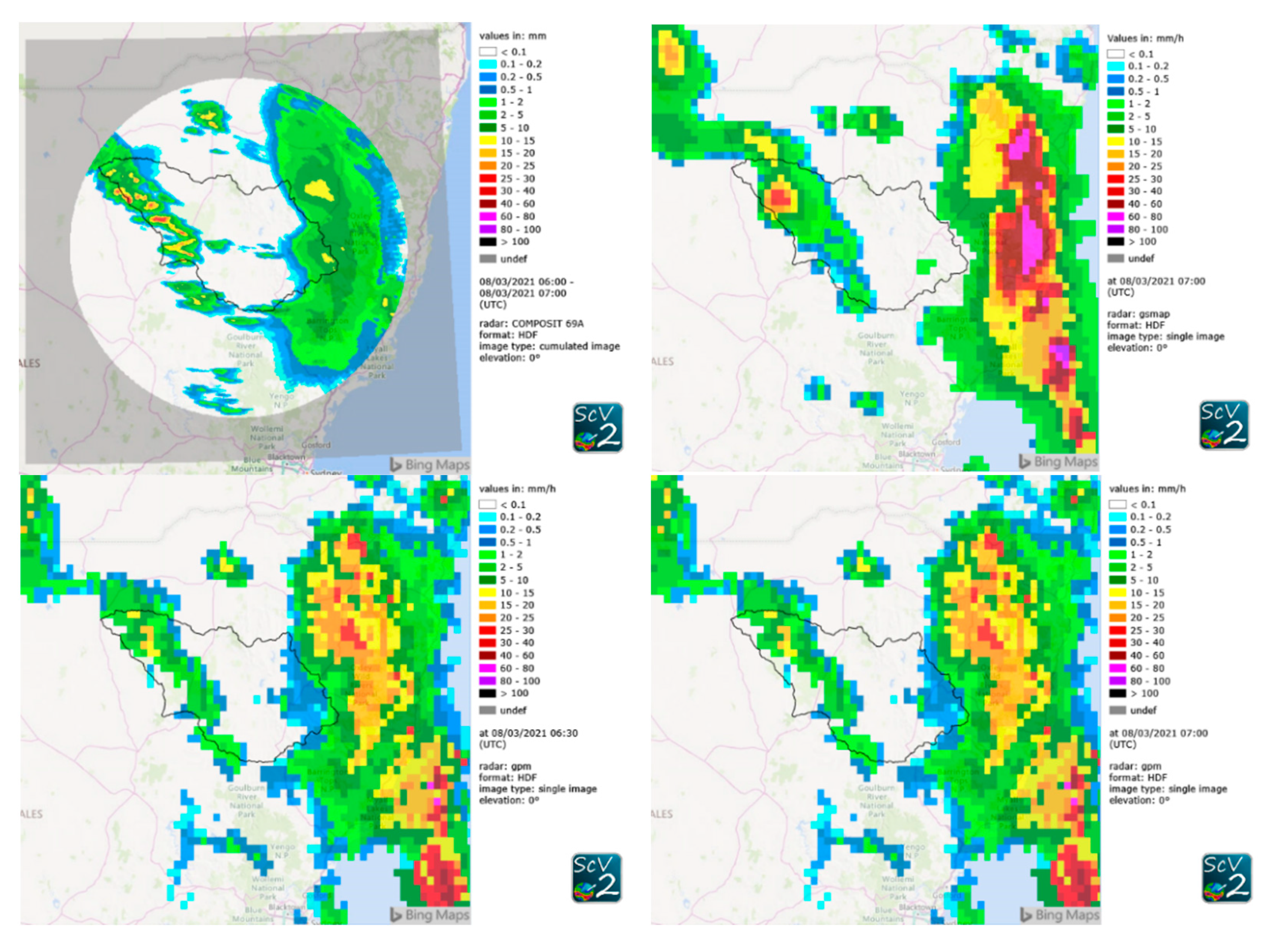
4.3. First Verification Results
Importing IMERG and GSMaP data into SCOUT allowed us to visualize the data on the same scale as the radar data. An example is shown in Figure 7, where the cumulated radar image on 3 August 2021 from 6 a.m. to 7 a.m. is shown along with GSMaP and IMERG data. For IMERG two snapshots are shown because of the half hourly resolution. Generally, the spatial structure is well captured in all datasets. As to be expected the radar data exhibits more spatial detail then IMERG and GSMaP. The magnitude of the precipitation intensities is similar in the eastern half of the image while significant differences can be found in the western part. Especially near the coast, the radar data (at a distance of more than 150 km from the radar) shows significantly less precipitation, which is likely caused by overshooting, such that in this area IMERG and GSMaP are superior to the radar data. However, there are also significant differences in the precipitation amounts of both satellite-based precipitation estimates in this region.
5. Discussion or the Way Ahead
5.1. Benchmark
The gauge adjusted radar data represent a well-suited precipitation dataset for the applications envisioned within WaterSENSE and are available in near real-time for the Namoi catchment. However, as radar and rain gauge data are not available or feasible to use everywhere, even in Australia, satellite-based precipitation products are explored. These datasets need to be analyzed further with the different requirements on the temporal and spatial resolution and accuracy in mind. The gauge adjusted radar data are an excellent benchmark for this purpose. Limitations of the satellite-based precipitation products such as the spatial resolution of the data will require further processing of the data.
5.2. Method Extensions: Use of Soil Moisture Data
One promising approach for improving the spatial resolution of the satellite-based precipitation products is to combine them with soil moisture inferred from EO data [19]. The basic idea is that soil acts as a natural rain gauge and hence soil moisture and its changes can be related to past rainfall. One advantage is that the EO measurements from which soil moisture is derived are completely different from the ones used for the precipitation products. Thus, soil moisture and precipitation are two independent datasets. The other advantage is the spatial resolution of the soil moisture, which greatly exceeds those of EO precipitation data. An algorithm which derives soil moisture from the Sentinel-1 satellites with a 1 km resolution is presented in [20]. Data based on this algorithm is made available operationally for Europe through the Copernicus initiative. It is explicitly noted that soil moisture changes due to precipitation are well captured. The authors of [21] have even derived soil moisture at a 500 m resolution. In WaterSENSE, soil moisture is derived as part of the water cycle monitoring toolkit. Different approaches exist to derive precipitation from EO soil moisture or to use soil moisture to improve the precipitation data: API [22] and in a modified version [23], SMART [24], SM2Rain [7], and PrIMS [25] more recently. In WaterSENSE, our approach is to use soil moisture to improve existing EO precipitation data, rather than deriving precipitation from soil moisture. This agrees with our modular approach of offering the highest quality data where and when available.
Other alternatives that will be explored are to integrate the satellite-based precipitation products with data from local rain gauges in near real-time. This yields the potential to make this data globally less uniform but locally more suitable for practical applications. In addition, the potential of increasing the spatial resolution of rain gauge-based gridded datasets with the help of soil moisture from EO data will be investigated.
6. Conclusions
A high-quality gridded precipitation dataset, based on radar and rain gauge data, was derived for the Namoi catchment. The quality of the data as well as the high temporal and spatial resolution are ideally suited for the hydrological and agricultural applications envisioned in WaterSENSE. However, as the availability of precipitation measurements by radar and rain gauge is very heterogeneous in Australia and in large parts of the world, different approaches need to be explored for less data-rich regions. Satellite based multi-instrument precipitation data such as GSMaP and IMERG present promising alternatives due to their near global availability. The quality of the EO precipitation data will be evaluated with the demands of WaterSENSE in mind. The gauged-adjusted radar data forms an ideal benchmark for this task. For improvements of the overall accuracy and especially the spatial resolution of the data, an approach using Copernicus EO soil moisture data will be investigated.
Author Contributions
Conceptualization, T.E. and A.S.; methodology, A.S.; software, T.E. and A.S.; validation, A.S.; formal analysis, A.S.; writing—original draft preparation, A.S.; visualization, A.S.; supervision, T.E.; project administration, T.E.; funding acquisition, T.E. All authors have read and agreed to the published version of the manuscript.
Funding
This research was funded by the Horizon 2020 research and innovation programme, grant number 870344.
Institutional Review Board Statement
Not applicable.
Informed Consent Statement
Not applicable.
Data Availability Statement
The processed radar data presented in this study are openly available in zenodo at https://0-doi-org.brum.beds.ac.uk/10.5281/zenodo.5602667. The Global Rainfall Map (GSMaP) data by JAXA Global Rainfall Watch was produced and distributed by the Earth Observation Research Center, Japan Aerospace Exploration Agency and is available under https://sharaku.eorc.jaxa.jp/GSMaP/ (accessed on 20 September 2021). The IMERG data were obtained from the NASA/Goddard Space FlightCenter, and accessed through jsimpsonftps.pps.eosdis.nasa.gov/imerg/early (accessed on 20 September 2021) and jsimpsonftps.pps.eosdis.nasa.gov/imerg/late (accessed on 20 September 2021) respectively.
Conflicts of Interest
The authors declare no conflict of interest.
References
- Einfalt, T.; Frerk, I. On the influence of high quality rain gauge data for radar-based rainfall estimation. In Proceedings of the 12th ICUD, Porto Alegre, Brazil, 11–16 September 2011. [Google Scholar]
- Willems, P.; Einfalt, T. Sensors for rain measurements. In Metrology in Urban Drainage and Stormwater Management: Plug and Pray; IWA Publishing: London, UK, 2021; Volume 11, pp. 11–33. [Google Scholar] [CrossRef]
- Huffman, G.J.; Bolvin, D.T.; Braithwaite, D.; Hsu, K.; Joyce, R.; Xie, P.; Yoo, S.H. Algorithm Theoretical Basis Document (ATBD) Version 06. NASA Global Precipitation Measurement (GPM) Integrated Multi-Satellite Retrievals for GPM (IMERG). 2019. Available online: https://pmm.nasa.gov/data-access/downloads/gpm (accessed on 4 December 2019).
- Kubota, T.; Aonashi, K.; Ushio, T.; Shige, S.; Takayabu, Y.N.; Kachi, M.; Arai, Y.; Tashima, T.; Masaki, T.; Kawamoto, N.; et al. Global Satellite Mapping of Precipitation (GSMaP) Products in the GPM Era. In Satellite Precipitation Measurement. Advances in Global Change Research; Levizzani, V., Kidd, C., Kirschbaum, D., Kummerow, C., Nakamura, K., Turk, F., Eds.; Springer: Cham, Switzerland, 2020; Volume 67, pp. 355–373. [Google Scholar] [CrossRef]
- Speirs, P.; Gabella, M.; Berne, A. A Comparison between the GPM Dual-Frequency Precipitation Radar and Ground-Based Radar Precipitation Rate Estimates in the Swiss Alps and Plateau. J. Hydrometeorol. 2017, 18, 1247–1269. [Google Scholar] [CrossRef]
- Joss, J.; Gabella, M.; Perona, G. Needs and expectations after the 1st VOLTAIRE workshop, Upscaling and consequences of non-homogeneous beam filling. In Proceedings of the 1st VOLTAIRE Workshop, Barcelona, Spain, 6–7 October 2003; pp. 6–8. [Google Scholar]
- Brocca, L.; Moramarco, T.; Melone, F.; Wagner, W. A new method for rainfall estimation through soil moisture observations. Geophys. Res. Lett. 2013, 40, 853–858. [Google Scholar] [CrossRef]
- Lanza, L.G.; Stagi, L. High resolution performance of catching type rain gauges from the laboratory phase of the WMO Field Intercomparison of Rain Intensity Gauges. Atmos. Res. 2009, 94, 555–563. [Google Scholar] [CrossRef]
- Sevruk, B. Niederschlag ALS Wasserkreislaufelement: Theorie und Praxis der Niederschlagsmessung; Boris Sevruk: Zürich, Switzerland, 2005. [Google Scholar]
- Kirstetter, P.E. Validating the Intrinsic Uncertainty: Implications for Hydrologic Applications; World Climate Research Programme: Geneva, Switzerland, 2021. [Google Scholar]
- NSW Department of Planning, Industry and Environment. Draft Regional Water Strategy—Namoi: Strategy. 2021. Available online: https://www.industry.nsw.gov.au/__data/assets/pdf_file/0009/354267/namoi-strategy.pdf (accessed on 17 September 2021).
- Einfalt, T.; Denoeux, T.; Jacquet, G. A radar rainfall forecasting method designed for hydrological purposes. J. Hydrol. 1990, 114, 229–244. [Google Scholar] [CrossRef]
- Gabella, M.; Notarpietro, R. Ground Clutter Characterization and Elimination in Mountainous Terrain. In Proceedings of the ERAD, Delft, The Netherlands, 18–22 November 2002; pp. 305–311. [Google Scholar]
- Bech, J.; Codina, B.; Lorente, J.; Bebbington, D. The Sensitivity of Single Polarization Weather Radar Beam Blockage Correction to Variability in the Vertical Refractivity Gradient. J. Atmos. Ocean. Technol. 2003, 20, 845–855. [Google Scholar] [CrossRef] [Green Version]
- Jasper-Tönnies, A.; Jessen, M. Improved radar QPE with temporal interpolation using an advection scheme. In Proceedings of the Eighth European Conference on Radar in Meteorology and Hydrology (ERAD), Garmisch-Partenkirchen, Germany, 3 August–1 September 2014. [Google Scholar]
- World Meteorological Organization. Guide to Meteorological Instruments and Methods of Observation, 7th ed.; WMO No. 8, Part II Observing Systems; WMO: Geneva, Switzerland, 2008; Chapter 9. [Google Scholar]
- Schellart, A.N.A.; Wang, L.; Onof, C. High resolution rainfall measurement and analysis in a small urban catchment. In Proceedings of the 9th International Workshop on Precipitation in Urban Areas: Urban Challenges in Rainfall Analysis (UrbanRain), St. Moritz, Switzerland, 6–9 December 2012. [Google Scholar]
- IPWG Global Precipitation Datasets. 2021. Available online: https://www.isac.cnr.it/~ipwg/data/datasets.html (accessed on 10 August 2021).
- Massari, C.; Camici, S.; Ciabatta, L.; Brocca, L. Exploiting satellite-based surface soil moisture for flood fore-casting in the Mediterranean area: State update versus rainfall correction. Remote Sens. 2018, 10, 292. [Google Scholar] [CrossRef] [Green Version]
- Bauer-Marschallinger, B.; Freeman, V.; Cao, S.; Paulik, C.; Schaufler, S.; Stachl, T.; Modanesi, S.; Massari, C.; Ciabatta, L.; Brocca, L.; et al. Toward Global Soil Moisture Monitoring with Sentinel-1: Harnessing Assets and Overcoming Obstacles. IEEE Trans. Geosci. Remote Sens. 2018, 57, 520–539. [Google Scholar] [CrossRef]
- Foucras, M.; Zribi, M.; Albergel, C.; Baghdadi, N.; Calvet, J.-C.; Pellarin, T. Estimating 500-m Resolution Soil Moisture Using Sentinel-1 and Optical Data Synergy. Water 2020, 12, 866. [Google Scholar] [CrossRef] [Green Version]
- Crow, W.T.; Huffman, G.J.; Bindlish, R.; Jackson, T.J. Improving Satellite-Based Rainfall Accumulation Estimates Using Spaceborne Surface Soil Moisture Retrievals. J. Hydrometeorol. 2009, 10, 199–212. [Google Scholar] [CrossRef] [Green Version]
- Pellarin, T.; Louvet, S.; Gruhier, C.; Quantin, G.; Legout, C. A simple and effective method for correcting soil moisture and precipitation estimates using AMSR-E measurements. Remote Sens. Environ. 2013, 136, 28–36. [Google Scholar] [CrossRef]
- Crow, W.T.; Berg, M.J.V.D.; Huffman, G.; Pellarin, T. Correcting rainfall using satellite-based surface soil moisture retrievals: The Soil Moisture Analysis Rainfall Tool (SMART). Water Resour. Res. 2011, 47, 576. [Google Scholar] [CrossRef]
- Pellarin, T.; Román-Cascón, C.; Baron, C.; Bindlish, R.; Brocca, L.; Camberlin, P.; Fernández-Prieto, D.; Kerr, Y.H.; Massari, C.; Panthou, G.; et al. The Precipitation Inferred from Soil Moisture (PrISM) Near Real-Time Rainfall Product: Evaluation and Comparison. Remote Sens. 2020, 12, 481. [Google Scholar] [CrossRef] [Green Version]
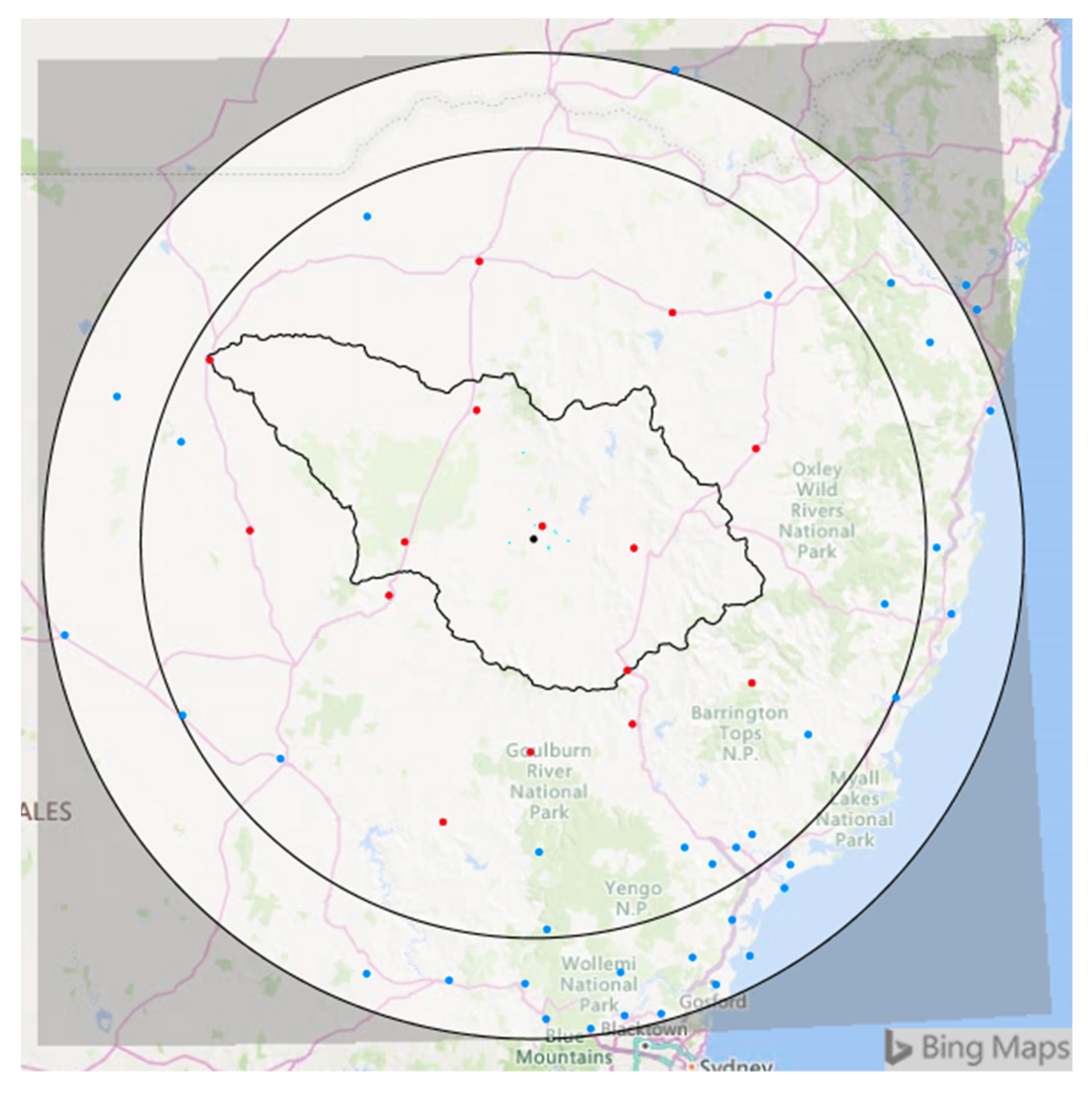
Figure 1.
Illustration of the radar range (bigger circle with 300 km radius) and the radar location (black dot) along with the Namoi catchment (black line) and station data not used (blue dots) and used in the adjustment process (red dots). The decreased range (240 km) selected for operational processing is indicated by the smaller black circle.

Figure 2.
Cumulated radar images for the period 17 April 2020 until 6 July 2020 for 0.5° (top left), 0.9° (top right) and 1.3° (bottom left). The data in the bottom right are the same as on the top right but after all corrections (beam blockage filter, reverse speckle filter, speckle filter, clutter map and Gabella filter) except for the advection correction and the radar-gauge adjustment have been applied to the data.
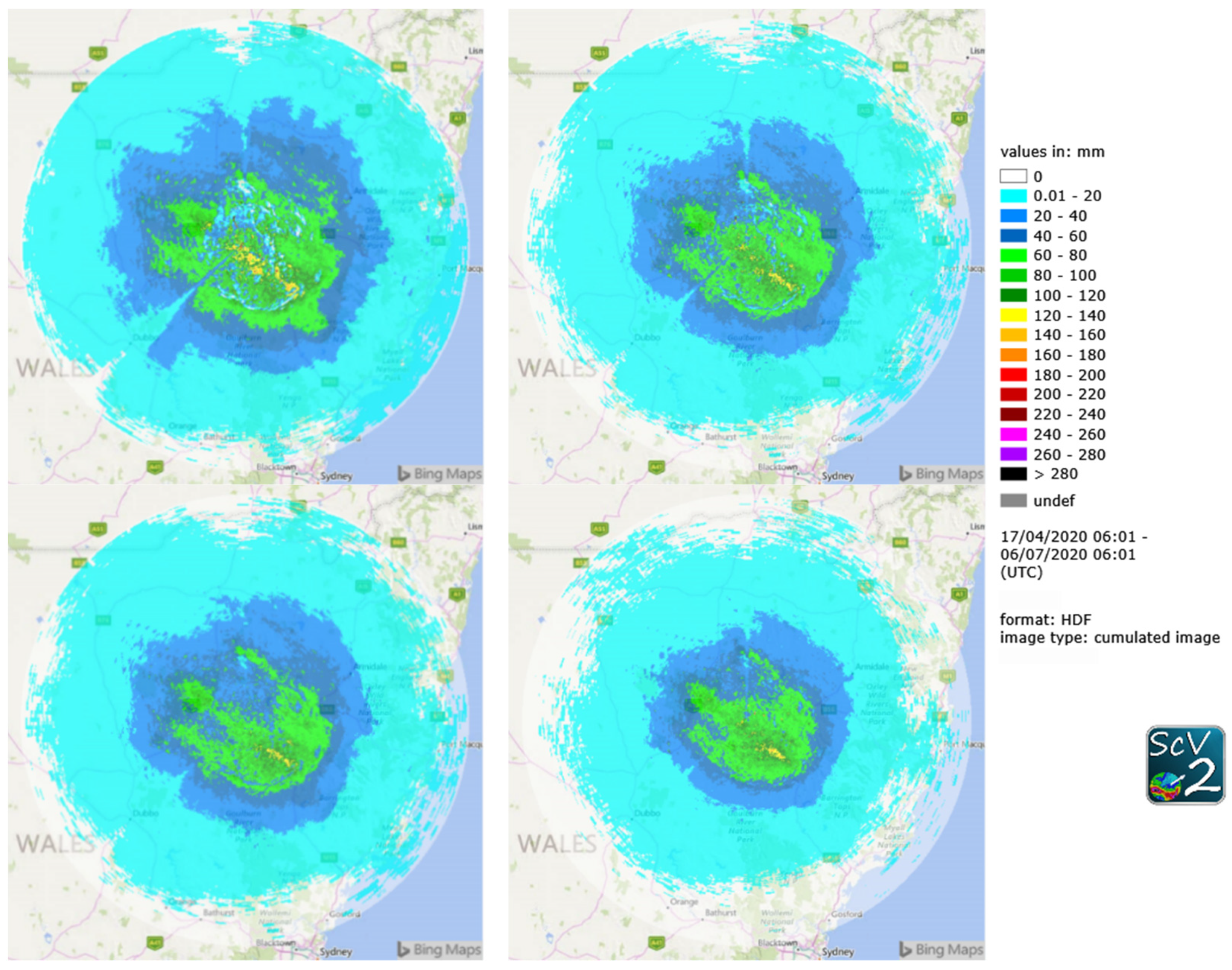
Figure 3.
A single radar image at 0.9° elevation before clutter removal (left) and afterwards (right).
Figure 3.
A single radar image at 0.9° elevation before clutter removal (left) and afterwards (right).
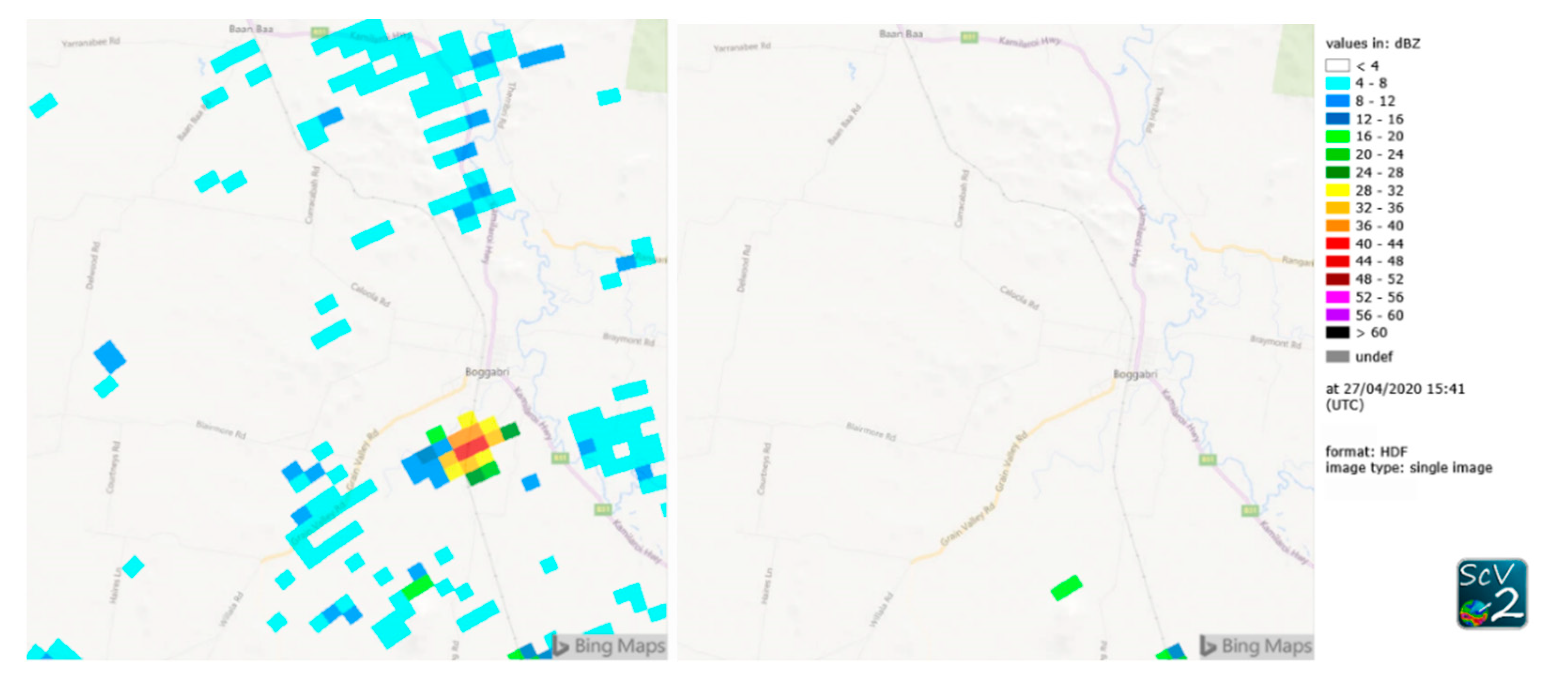
Figure 4.
A single radar image at 0.9° elevation before the holes in the precipitation field were (partially) filled (left) and afterwards (right).
Figure 4.
A single radar image at 0.9° elevation before the holes in the precipitation field were (partially) filled (left) and afterwards (right).

Figure 5.
A single radar image at 0.9° elevation before the advection correction was applied (left) and afterwards (right).
Figure 5.
A single radar image at 0.9° elevation before the advection correction was applied (left) and afterwards (right).
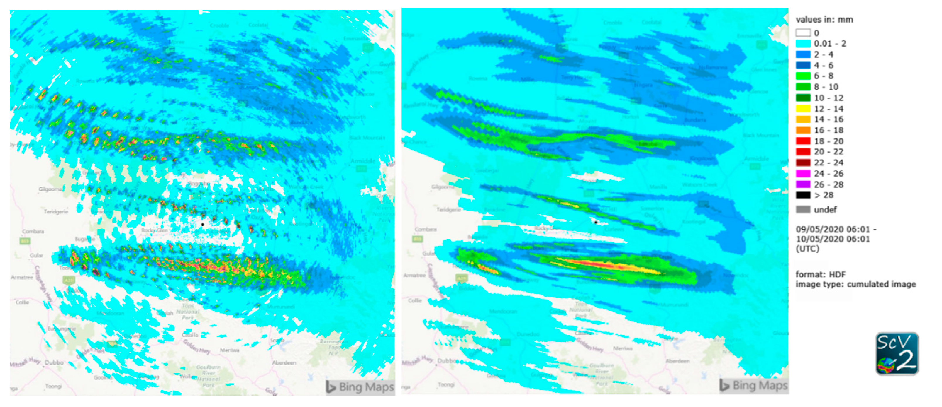
Figure 6.
Cumulated radar image before corrections (upper left), after all corrections (upper right), and including the radar-gauge adjustment (lower left).
Figure 6.
Cumulated radar image before corrections (upper left), after all corrections (upper right), and including the radar-gauge adjustment (lower left).
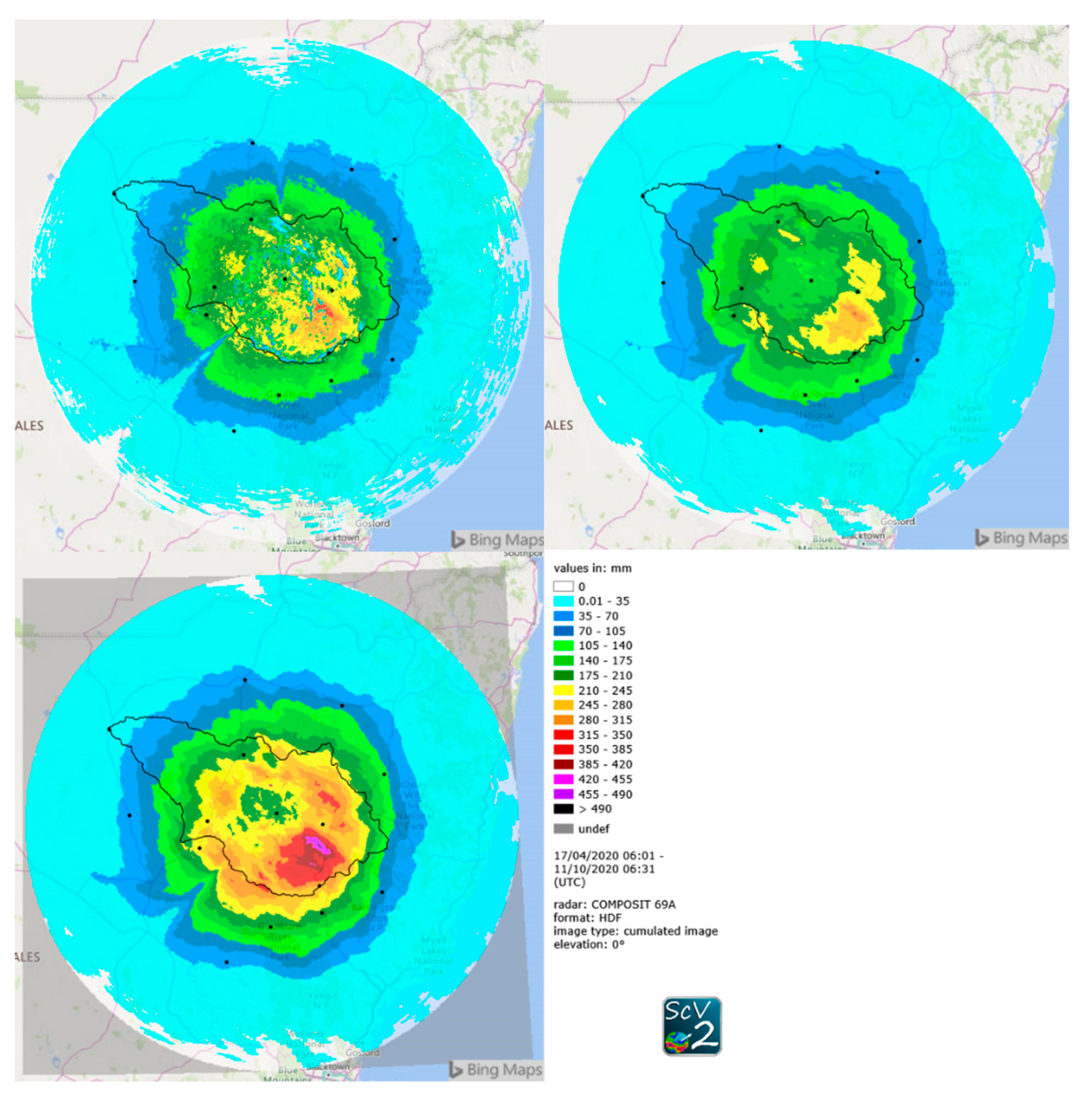
Figure 7.
Illustrative comparison of cumulated data of Namoi radar (upper left) with snapshots of GSMaP (upper right) and IMERG (bottom).
Figure 7.
Illustrative comparison of cumulated data of Namoi radar (upper left) with snapshots of GSMaP (upper right) and IMERG (bottom).

Table 1.
Specification of the polar volume radar data of the Namoi radar prior and after October 2020.
Table 1.
Specification of the polar volume radar data of the Namoi radar prior and after October 2020.
| Prior October 2020 | After October 2020 | |
|---|---|---|
| Elevations | 0.5°, 0.9°, 1.3° and higher elevations not considered here | 0.5°, 0.8°, 1.4° and higher elevations not considered here |
| Azimut resolution | 1° | 1° |
| Radial resolution | 500 m | 250 m |
| Nominal radius | 300 km | 300 km |
| Reflectivity resolution | 159 dBZ-classes | 159 dBZ-classes |
Publisher’s Note: MDPI stays neutral with regard to jurisdictional claims in published maps and institutional affiliations. |
© 2021 by the authors. Licensee MDPI, Basel, Switzerland. This article is an open access article distributed under the terms and conditions of the Creative Commons Attribution (CC BY) license (https://creativecommons.org/licenses/by/4.0/).
Share and Cite
MDPI and ACS Style
Strehz, A.; Einfalt, T. Precipitation Data Retrieval and Quality Assurance from Different Data Sources for the Namoi Catchment in Australia. Geomatics 2021, 1, 417-428. https://0-doi-org.brum.beds.ac.uk/10.3390/geomatics1040024
AMA Style
Strehz A, Einfalt T. Precipitation Data Retrieval and Quality Assurance from Different Data Sources for the Namoi Catchment in Australia. Geomatics. 2021; 1(4):417-428. https://0-doi-org.brum.beds.ac.uk/10.3390/geomatics1040024
Chicago/Turabian StyleStrehz, Alexander, and Thomas Einfalt. 2021. "Precipitation Data Retrieval and Quality Assurance from Different Data Sources for the Namoi Catchment in Australia" Geomatics 1, no. 4: 417-428. https://0-doi-org.brum.beds.ac.uk/10.3390/geomatics1040024