
Good Statistical Practices for Contemporary Meta-Analysis: Examples Based on a Systematic Review on COVID-19 in Pregnancy


Department of Statistics, Florida State University, Tallahassee, FL 32306, USA
*
Author to whom correspondence should be addressed.
BioMedInformatics 2021, 1(2), 64-76; https://0-doi-org.brum.beds.ac.uk/10.3390/biomedinformatics1020005
Submission received: 26 May 2021
/
Revised: 8 July 2021
/
Accepted: 19 July 2021
/
Published: 23 July 2021
Abstract
:Systematic reviews and meta-analyses have been increasingly used to pool research findings from multiple studies in medical sciences. The reliability of the synthesized evidence depends highly on the methodological quality of a systematic review and meta-analysis. In recent years, several tools have been developed to guide the reporting and evidence appraisal of systematic reviews and meta-analyses, and much statistical effort has been paid to improve their methodological quality. Nevertheless, many contemporary meta-analyses continue to employ conventional statistical methods, which may be suboptimal compared with several alternative methods available in the evidence synthesis literature. Based on a recent systematic review on COVID-19 in pregnancy, this article provides an overview of select good practices for performing meta-analyses from statistical perspectives. Specifically, we suggest meta-analysts (1) providing sufficient information of included studies, (2) providing information for reproducibility of meta-analyses, (3) using appropriate terminologies, (4) double-checking presented results, (5) considering alternative estimators of between-study variance, (6) considering alternative confidence intervals, (7) reporting prediction intervals, (8) assessing small-study effects whenever possible, and (9) considering one-stage methods. We use worked examples to illustrate these good practices. Relevant statistical code is also provided. The conventional and alternative methods could produce noticeably different point and interval estimates in some meta-analyses and thus affect their conclusions. In such cases, researchers should interpret the results from conventional methods with great caution and consider using alternative methods.
1. Introduction
Systematic reviews and meta-analyses have been widely used to synthesize results from multiple studies on the same research topic in medical sciences [1,2]. The reliability of the synthesized evidence depends critically on appropriate methods used to perform meta-analyses [3,4]. However, despite the mass production of meta-analyses, it has been found that many meta-analyses need improvements in their methodological quality [5,6,7,8,9,10]. This is a particularly crucial issue in the COVID-19 pandemic because of the concerns about the expedited peer-review process [11,12,13,14].
This article uses a systematic review on COVID-19, recently published in The BMJ, to illustrate some good practices for performing a meta-analysis from statistical perspectives. Many non-statistical recommendations and quality assessments for a systematic review and meta-analysis can be found in the PRISMA (Preferred Reporting Items for Systematic Reviews and Meta-Analyses) checklists [3,15,16], the GRADE (Grading of Recommendations Assessment, Development and Evaluation) approaches [17,18], the AMSTAR (A MeaSurement Tool to Assess systematic Reviews) tools, etc. [19,20]. In recent years, meta-analyses have begun to adopt these non-statistical recommendations, but there is still much room for improvement in terms of statistical analyses.
For example, several papers pointed out that the well-known statistical method for the random-effects meta-analysis proposed by DerSimonian and Laird [21] is suboptimal [22,23,24]. Various methods with potentially better performance are available and can be readily implemented with various statistical software programs [25,26,27,28,29]. Nevertheless, the DerSimonian–Laird (DL) method continues to dominate contemporary meta-analyses [9]. Some popular software programs for meta-analysis (e.g., Review Manager) use the DL method as the default and perhaps the only option.
In this article, based on the aforementioned systematic review on COVID-19, we aim at exploring potential issues when using statistical methods for its meta-analyses and illustrating potential better alternatives. Reproducible code for all analyses is provided. We hope these materials will help practitioners accurately use appropriate statistical methods to perform high-quality meta-analyses in the future.
2. Case Study
We use the data of meta-analyses reported by Allotey et al. [30] as our examples. This study conducted a living systematic review, which will be updated periodically to incorporate evidence from new studies. We use the version of update 1 of the original article published on 1 September 2020. The systematic review identified a total of 192 studies and performed multiple meta-analyses to investigate the prevalence, clinical manifestations, risk factors, and maternal and perinatal outcomes in pregnant and recently pregnant women (henceforth, pregnant women) with COVID-19. We select this systematic review for illustrations due to several considerations. It deals with the important research topic of COVID-19, where the appropriate use of statistical analyses is particularly crucial for timely and accurate decision-making. Also, this review covers a wide range of meta-analysis settings; the included meta-analyses had diverse outcomes, types of studies (non-comparative and comparative), numbers of studies, sample sizes, extents of heterogeneity, etc.
This article uses three meta-analyses from this systematic review to illustrate several statistical advances. The first two meta-analyses synthesize comparative studies; their outcomes are fever and cough in pregnant women compared with non-pregnant women of reproductive age with COVID-19. Each meta-analysis contains 11 studies. The original meta-analysis on fever yielded a pooled odds ratio (OR) of 0.49 with 95% confidence interval (CI) (0.38, 0.63) and = 40.8% suggesting moderate heterogeneity. The original meta-analysis on cough yielded a pooled OR of 0.72 with 95% CI (0.50, 1.03) and = 63.6% suggesting moderately high heterogeneity. Overall, pregnant women with COVID-19 were less likely to have fever and cough than non-pregnant women with COVID-19. The association with fever was statistically significant, while that with cough was not. For illustrative purposes, Figure 1 shows the forest plot of the meta-analysis on cough.
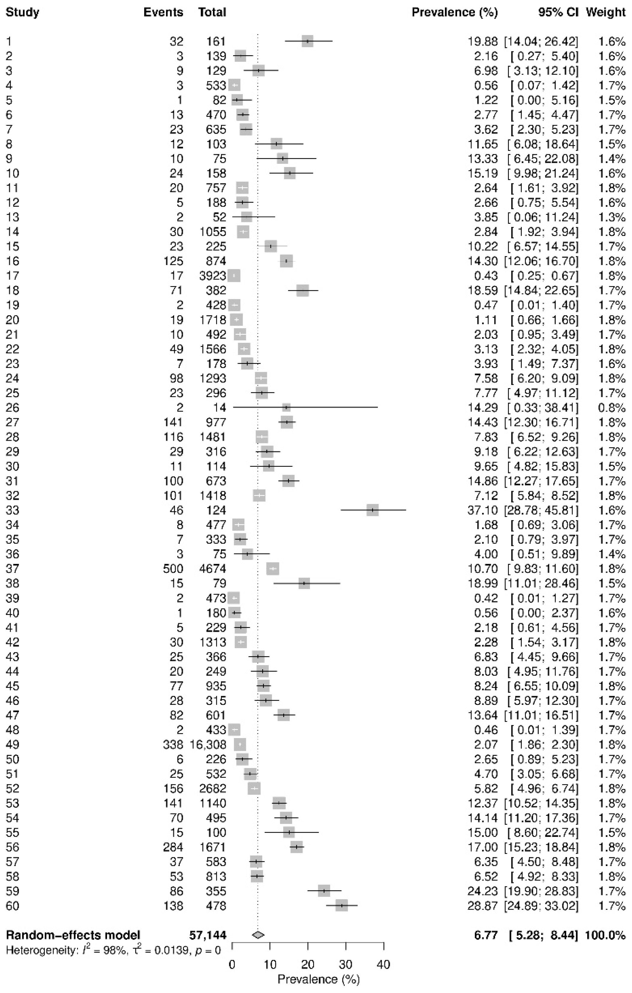
The third meta-analysis combines non-comparative data from 60 studies to obtain a pooled prevalence of COVID-19 in pregnant women; Figure 2 presents its forest plot. The original analysis gave a pooled prevalence of 7% with 95% CI (5%, 8%) and = 98.0% suggesting extremely high heterogeneity.
3. Good Practices
3.1. Providing Sufficient Information of Included Studies
Meta-analysts should provide sufficient information of included studies so that peer reviewers and other researchers could reproduce the meta-analyses and validate the results. The PRISMA statement and its extensions give comprehensive overviews of the reporting of meta-analyses [15,16,31,32]; meta-analysts are advised to carefully follow these guidelines for general purposes. Here, we focus on the reporting from statistical perspectives; the non-statistical parts (e.g., study selection) are not discussed, while they are equally critical for validating meta-analyses. The statistical data from individual studies can be feasibly provided in meta-analyses of aggregate data. However, this practice may be challenging for meta-analyses of individual participant data (IPD), which could involve concerns about data privacy. In such situations, meta-analysts may provide detailed procedures with other researchers to apply for access to the de-identified participant-level data. In the following, we restrict the discussions to meta-analyses of aggregate data.
In all three examples, the meta-analyses use aggregate data, i.e., the number of subjects with fever or cough and the sample sizes of pregnant and non-pregnant women in the comparative studies, and the number of cases of COVID-19 and the sample size of pregnant women in the prevalence data. These aggregate data are transparently provided by Allotey et al. [30], displayed in the corresponding forest plots; see, e.g., Figure 1 and Figure 2. With these data available, we can reproduce the results, such as the prevalence and OR, of each individual study. They also permit us to employ alternative meta-analysis methods (detailed later).
3.2. Providing Information for Reproducibility of Meta-Analyses
In addition to the information of individual studies, reproducibility of meta-analyses also requires transparency in the statistical analyses, including the choice of measures for quantifying the study results, models for pooling the individual-study data, methods for assessing heterogeneity between studies and small-study effects, software program and its version used for performing the analyses, as well as subgroup analyses and sensitivity analyses (if applicable).
For example, Allotey et al. [30] specified that the OR was used for pooling the comparative dichotomous data with random-effect models. If comparative continuous data are needed to be pooled with dichotomous data, the standardized mean difference was used as the effect measure of the continuous data and was transformed to the log OR using the method by Chinn [33]. For the prevalence data, the Freeman–Tukey double-arcsine transformation was applied to the proportion estimate from each study to stabilize its sample variance [34]. The authors used the statistic to assess heterogeneity [35,36], but they did not assess small-study effects or publication bias. When the random-effects model is used, it is also critical to specify the estimator of the between-study variance, which is a key parameter in this model and could greatly affect the pooled results, particularly 95% CIs. The authors only specified that the DL method was used for pooling prevalence data but did not specify that for pooling comparative data. We have reproduced their meta-analyses of comparative data and found that the DL method was also used for comparative data. The original meta-analyses were all performed with Stata 16, which is widely used in the current literature of meta-analyses.
3.3. Using Appropriate Terminologies
Based on our knowledge, it was not uncommon that some inappropriate terminologies were used for meta-analysis methods. For example, in the systematic review by Allotey et al. [30], the prevalence was incorrectly referred to as “rate ratio” in the meta-analyses of prevalence (Figures 2 and 3 in the original article). As its name suggests, the rate ratio is a ratio of incidence rates for comparative studies, while the prevalence (or proportion) is a type of non-comparative data. The incidence rate also includes certain time elements (e.g., person-year), while the prevalence does not include such elements.
Besides these minor issues in this case study, Ioannidis [37] explored the problem of massive citations in detail. Additional examples include referring to the forest plot [38] as ‘‘Forrest plots”, “honoring the nonexistent Dr. Forrest,” and the funnel plot [39,40]. for assessing small-study effects as “Beggar’s funnel plot,” “apparently copy-pasting from some original source(s) that mistyped Colin Begg’s funnel plot.” Moreover, the commonly used Q test for heterogeneity is often referred to as the “Cochrane’s Q” or “Cochran’s Q.” The former wrongly relates the Q test to the Cochrane Collaboration. The latter is used in many meta-analyses due to the paper by William G. Cochran [41], although it was not designed for testing for heterogeneity in Cochran’s original work [42].
In order to use appropriate statistical methods for a meta-analysis, the first step is to specify their names correctly. When referring to certain meta-analysis methods, we suggest researchers always reading and citing the original methodological articles or tutorials that proposed, introduced, or reviewed the methods.
3.4. Double-Checking Presented Results
A meta-analysis has the power to yield more precise results than individual studies, but it could also inherit potential research errors from individual studies. It may be difficult to discover and correct the errors hidden in individual studies. The potential erroneous results from suspectable studies could be removed from the meta-analysis, or sensitivity analyses could be conducted to evaluate such studies’ impact on the pooled results.
Additional errors could occur when pooling the individual studies; researchers should try their best to avoid such errors when inputting the data and outputting the results. For example, a systematic review team may assign two or more researchers to independently extract individual studies’ data, perform meta-analyses, check the results, and proofread the final manuscript. With sufficient information provided, it is more likely to check for potential internal reporting discrepancies. Several examples of internal reporting discrepancies are discussed by Puljak et al. [43].
Taking the systematic review by Allotey et al. [30] as an example, several discrepancies appeared. In the meta-analysis on fever comparing pregnant women with non-pregnant women with COVID-19 (Figure 5 in the original article), the OR of the study “Wei L 2020” was reported as 0.40 with 95% CI (0.11, 0.77), and the OR of another study “Wang Z 2020” was reported as 0.29 with 95% CI (0.11, 0.77). The reported CIs were identical, while the point estimates of the ORs were different, and the CIs were displayed differently in the forest plot. Based on the forest plot, the CI of “Wei L 2020” encompassed the null value 1, so the reported CI of this study was likely erroneous when copying and pasting the numeric results in the forest plot. Fortunately, because the event counts and sample sizes (8 and 17 for pregnant women and 18 and 26 for non-pregnant women) were reported for this study, we can derive the correct 95% CI as (0.11, 1.40). A similar issue occurred in the study “Zambrano LD 2020,” whose OR was reported as 0.52 with 95% CI (0.50, 0.50). The CI did not even encompass the point estimate; again, this was likely due to a typesetting error. In the meta-analysis on cough (also Figure 5 in the original article), the total sample sizes of pregnant and non-pregnant women across the 11 studies were reported as 5468 and 75,053, respectively. These total sample sizes were also apparently erroneous because they are smaller than the sample sizes in the single study “Zambrano LD 2020.” The correct total sample sizes should be 17,806 and 222,493 (Figure 1).
3.5. Considering Alternative Estimators of Between-Study Variance
As mentioned earlier, the example meta-analyses were performed with the random-effects model, and the well-known DL method was used to estimate the between-study variance. The DL estimator is based on the method of moments. This method is popular possibly because it is a simple, non-iterative method with a closed-form [21]. Many alternative estimators have been proposed for the between-study variance [44,45,46]. Although the DL estimator retains its usefulness in some situations (e.g., large sample sizes) [22], it could bias the estimated between-study variance, and the restricted maximum-likelihood (REML) estimator generally performs better among various frequentist methods [25,26,47]. Bayesian methods can also be good alternatives as they have the ability to incorporate prior information (e.g., from external evidence or experts’ opinions) in the final estimates [48,49]. The method used to estimate heterogeneity plays a crucial role in a meta-analysis because it could greatly affect the estimated overall effect, particularly the width of its CI and thus the statistical significance. Therefore, we suggest researchers exploring alternative options for estimating the between-study variance offered by the software programs used for their meta-analyses. In many cases, the alternative estimators may produce similar results to the DL estimator, and the DL estimator may be considered reliable. However, if these estimators yield fairly different results, researchers may consider alternative estimators.
In the example meta-analysis on fever, the DL method estimated the between-study variance as 0.053, leading to an overall OR estimate of 0.488 with 95% CI (0.377, 0.632). Using the REML method, the estimate became 0.127, leading to an overall OR estimate of 0.453 with 95% CI (0.326, 0.629). In the example meta-analysis on cough, the DL method estimated the between-study variance as 0.168, leading to an overall OR estimate of 0.719 with 95% CI (0.502, 1.031). Using the REML method, the estimate became 0.239, leading to an overall OR estimate of 0.711 with 95% CI (0.476, 1.061).
3.6. Considering Alternative Confidence Intervals
Conventionally, the CI of the overall estimate in a meta-analysis is produced assuming normality (e.g., for the log OR). However, this normality assumption might be questionable in some situations [50]; as such, the normality-based CI may not have the desired coverage probability (e.g., 95%). Hartung and Knapp [51,52] and Sidik and Jonkman [53,54] independently introduced a refined CI based on the t-distribution for the random-effects meta-analysis. This t-based CI has been shown to have better coverage probabilities than the standard normality-based CI by various simulation studies, particularly when a meta-analysis only contains a few studies [29,55,56,57]. Of note, this CI was designed for the random-effects meta-analysis, and it is inappropriate to apply it to the fixed-effect (also known as common-effect) meta-analysis that assumes no heterogeneity.
The t-based 95% CI of the overall OR in the example meta-analysis on fever was (0.352, 0.678) and (0.316, 0.650) using the DL and REML methods, respectively, both wider than their counterparts of normality-based 95% CIs (0.377, 0.632) and (0.326, 0.629). Similarly, in the example meta-analysis on cough, the t-based 95% CI of the overall OR was (0.463, 1.118) and (0.453, 1.114) using the DL and REML methods, respectively. Also, both were wider than their counterparts of normality-based 95% CIs (0.502, 1.031) and (0.476, 1.061).
3.7. Reporting Prediction Intervals
Heterogeneity between studies frequently appears and is generally expected in a meta-analysis [58]. Standard meta-analysis approaches use the random-effects model to account for the heterogeneity and use the estimated between-study variance and/or the statistic to quantify it. However, it is difficult to apply these metrics to clinical practice for future research. Over the last decade, much effort has been made to promote the reporting of the prediction interval (PI) in a meta-analysis, but only a small proportion of meta-analyses adopt this recommendation in the current literature [9,59,60,61,62,63]. The PI represents the expected range of the true effects in future studies, making it easier to apply meta-analysis results to clinical practice. The PI is wider than the CI due to the heterogeneity between existing studies in a meta-analysis and future studies. A meta-analysis may have a CI not encompassing the null value (thus implying a statistically significant effect), but its PI could encompass the null, indicating that a future study could have opposite results [64].
Despite the attractive features of the PI, researchers should note that the PI could be subject to large uncertainties when the number of studies in a meta-analysis is relatively small (e.g., <10). In the presence of small-study effects (detailed in the following subsection), the PI could have poor coverage due to biased estimates. Therefore, the PI should be interpreted with caution in these situations. Also, the PI is designed for a random-effects meta-analysis; it is not sensible for a fixed-effect meta-analysis.
In the example meta-analysis on fever, based on the REML estimator of the between-study variance, the 95% PI of the overall OR is (0.186, 1.104), encompassing the null value 1. Recall that the 95% CI of this meta-analysis is (0.326, 0.629), not encompassing 1. Therefore, although the meta-analysis concludes a statistically significant association between fever and pregnancy, this conclusion could be changed in a new study.
In the example meta-analysis on cough, based on the REML estimator of the between-study variance, the 95% PI of the overall OR is (0.214, 2.356), much wider than its 95% CI (0.476, 1.061). The PI can be incorporated into the forest plot [60,65], as shown in Figure 1. Of note, the results in Figure 1 were produced using the DL method to reproduce the original results in Allotey et al. [30], so the interval estimates were different from the foregoing results based on the REML method.
3.8. Assessing Small-Study Effects Whenever Possible
Small-study effects refer to the phenomenon that smaller studies containing fewer subjects have substantially different results from larger studies with more subjects. They could be caused by publication bias, when small studies with statistically significant findings or effect estimates in the desired direction are more likely published in the literature than those with non-significant findings or effect estimates in the opposite direction [66,67]. Assessing small-study effects is a crucial step for validating the synthesized evidence from a meta-analysis; if substantial small-study effects appear, the certainty of the synthesized evidence should be rated down [3,68,69]. Common approaches to assessing small-study effects include graphical tools, such as the funnel plot [39,40], and quantitative methods, such as Egger’s test, Begg’s test, and skewness [70,71,72,73,74]. The asymmetry in a funnel plot is an indicator of potential small-study effects. Additional contours that depict areas of various statistical significance levels can be further added to the usual funnel plot, referred to as the contour-enhanced funnel plot [40,75,76]. They help distinguish publication bias from other potential factors (e.g., subgroup effects) that might cause small-study effects.
We assessed small-study effects in the meta-analyses on fever and cough. Figure 3 presents their contour-enhanced funnel plots, where the contours represent the commonly used statistical significance levels at 0.01, 0.05, and 0.1.
In Figure 3A, the funnel plot shows that the (log) ORs from the 11 studies on fever were distributed asymmetrically. Smaller studies with larger standard errors tended to have smaller ORs away from the null value 1, indicating small-study effects. The potential missing studies at the lower right part of the funnel plot are likely located within the white area with p-values > 0.1. Therefore, this contour-enhanced funnel plot supports the existence of publication bias. Nevertheless, the p-value of Egger’s test was 0.275, suggesting that publication bias was not statistically significant. Of note, if the potential missing studies were located in areas with very small p-values, then the small-study effects may not be explained by publication bias. In such cases, meta-analysts are encouraged to explore the factors that might cause the funnel plot’s asymmetry, e.g., by performing subgroup analyses to examine whether the asymmetry was attributable to heterogeneity [40,77].
Although small-study effects were not statistically significant based on Egger’s test in this case study, it did not mean that the assessment of small-study effects was unnecessary. Statistical methods for detecting small-study effects usually have low powers, particularly in meta-analyses with only a few studies. As such, the significance level for detecting small-study effects is typically set to 0.1, higher than the most popular cutoff of 0.05 [78]. Here, meta-analysts should distinguish the p-value of tests for small-study effects from the p-values of individual studies’ effect estimates. The significance levels depicted in the contour-enhanced funnel plot are intended for the latter. In addition, if a meta-analysis contains less than 10 studies, it might be inappropriate to use the funnel plot to detect small-study effects because it is hard to distinguish chance from real asymmetry [40].
In Figure 3B, the funnel plot for the meta-analysis on cough does not show apparent missing studies in the white area of non-significance. Therefore, it does not support the existence of publication bias.
3.9. Considering One-Stage Methods
Conventionally, meta-analyses are performed with two-stage methods; that is, within-study estimates are first obtained, and then the study-specific estimates are pooled together as an overall estimate. The two-stage methods are usually simple and intuitive; the study-specific estimates provided by them are also necessary for producing the forest plot for visualizing a meta-analysis and the funnel plot for assessing small-study effects. Nevertheless, they suffer from several limitations. First, the study-specific estimates in the two-stage methods are typically assumed to approximately follow normal distributions. For this purpose, certain transformations are applied to the original effect measures. For example, the OR is typically analyzed on the logarithmic scale, and the Freeman–Tuckey double-arcsine transformation is widely used to transform proportion estimates, as in the original analyses by Allotey et al. [30]. The transformed estimates may approximately follow normal distributions when the sample sizes are sufficiently large, while the approximation may be inaccurate for studies with small sample sizes [50]. In recent years, there are also growing concerns about the appropriateness of the Freeman–Tuckey double-arcsine transformation for meta-analyses of proportions [79,80,81]. Second, the variances of the effects from individual studies need to be estimated in the two-stage methods, and the estimated within-study variances are typically treated as fixed variables. Again, this practice may be valid for large-sample settings, but it is questionable for studies with small sample sizes [57]. For example, the (log) OR’s variance depends on the event counts, which are actually random variables instead of fixed variables. The (log) OR and variance are thus intrinsically associated, and such association could lead to non-negligible biases for small sample sizes and/or low even rates [82,83,84].
With the recent development of statistical methods for meta-analysis, many software programs have commands to pool data via one-stage methods, such as generalized linear mixed models (GLMM) and Bayesian hierarchical models. The one-stage methods assume exact likelihood functions for the observed data (e.g., the binomial likelihood for the event count from a group of patients). They do not need the estimation for each individual study and thus avoid some unrealistic assumptions made by the two-stage methods. Moreover, these methods are widely applicable to many types of meta-analyses, including comparative studies, proportions, and diagnostic tests [27,85,86,87,88,89,90]. In the following, we illustrate the use of GLMMs and Bayesian hierarchical models with two example meta-analyses.
In the meta-analysis on cough, recall that the overall OR was 0.719 with 95% CI (0.502, 1.031) based on the original analysis (the DL estimation) by Allotey et al. [30]; it was 0.711 with 95% CI (0.476, 1.061) using the REML estimation. We re-analyzed this dataset using the GLMM and Bayesian hierarchical models with a logit link function. For the Bayesian models, we used the vague normal prior N(0, 1002) for the overall log OR and the uniform prior U(0, 5) for the between-study standard deviation . We also considered the informative log-normal prior LN(2.89, 1.912) for , which was derived by Turner et al. [48] based on a large Cochrane database. The GLMM estimated the overall OR as 0.710 with 95% CI (0.493, 1.022). The Bayesian model with U(0, 5) prior for produced the estimated OR of 0.701 with 95% credible interval (CrI) (0.415, 1.143), and that with LN(2.89, 1.912) prior for gave 0.709 with 95% CrI (0.462, 1.047).
In the meta-analysis of the prevalence of COVID-19 in pregnant women, we re-analyzed it using the GLMM and Bayesian model with a logit link function, in addition to the original two-stage method used by Allotey et al. [30] (i.e., the DL estimation with the Freeman–Tuckey double-arcsine transformation). Based on the original two-stage method, the overall prevalence was estimated as 6.77% with 95% CI (5.28%, 8.44%). Based on the GLMM, the estimated overall prevalence became 5.44% with 95% CI (4.09%, 7.19%). The Bayesian model with U(0, 5) for produced the estimated OR of 5.44% with 95% CrI (4.04%, 7.34%). The prevalence estimates by both one-stage methods were smaller than those by the two-stage method by over 1%.
4. Conclusions
This article provided a summary of good practices for performing a meta-analysis from statistical perspectives. We illustrated these practices using meta-analyses published in a recent systematic review on COVID-19 in pregnancy. We hope they may help improve the methodological quality of future meta-analyses. For facilitating researchers to implement the methods reviewed in this article, the Supplemental File gives all code for our analyses.
Due to the urgent need for COVID-19 research, it has been dramatically expedited to conduct and peer-review meta-analyses. Nevertheless, it is critical to safeguard the integrity of scientific evidence during this challenging period of accelerated publishing [14]. This article shows that some statistical methods used in the example meta-analyses may be suboptimal. In our re-analyses with better alternatives, some meta-estimates had noticeable changes. Also, potential small-study effects might exist. Extra attention is needed to examine whether such effects might continue to exist in the future updates of this living systematic review after including new studies.
This article has several limitations because we were only able to focus on select statistical advances for meta-analysis based on a single case study on COVID-19. For example, for assessing small-study effects or publication bias, some selection models may be applied as sensitivity analyses to examine the robustness of synthesized results to potential bias [91,92]. Alternative meta-analysis methods are available to offer some benefits over the traditional fixed-effect and random-effects models under specific cases [93,94,95]. In addition, the current literature has debates on the choice of effect measures, e.g., relative risk, in meta-analyses [96,97]. This article has also not covered topics on meta-analyses of diagnostic tests [98]. All examples are meta-analyses of aggregate data, while meta-analyses of IPD may involve additional issues and require specific methods [99]. For a more comprehensive review of meta-analysis methods, one may refer to the Cochrane Handbook [100].
Systematic reviews and meta-analyses are a type of transdisciplinary research. Therefore, in addition to many statistical considerations reviewed in this article, non-statistical guidance is also crucial for conducting high-quality meta-research. For example, heterogeneity between studies may be assessed beyond the statistical perspectives [101]. To aid the statistical assessment of small-study effects, researchers are suggested to search for relevant unpublished studies (e.g., on preprint servers and trial registries), include them in meta-analyses, and explore their potential differences from the published studies [100]. Of course, because the unpublished studies are not peer-reviewed, they could be subject to a high risk of bias. The risk of bias must be carefully appraised if incorporating such studies in the systematic review [102].
Supplementary Materials
The following are available online at https://0-www-mdpi-com.brum.beds.ac.uk/article/10.3390/biomedinformatics1020005/s1: code for producing the results presented in the main content.
Funding
This research received no external funding.
Institutional Review Board Statement
Ethical review and approval were waived for this study because we focused on statistical methods for meta-analysis and used published data.
Informed Consent Statement
Patient consent was waived because this study used published data.
Data Availability Statement
The Supplementary Materials include the data used in this study.
Conflicts of Interest
The authors declare no conflict of interest.
References
- Berlin, J.A.; Golub, R.M. Meta-analysis as evidence: Building a better pyramid. JAMA 2014, 312, 603–606. [Google Scholar] [CrossRef] [PubMed]
- Gurevitch, J.; Koricheva, J.; Nakagawa, S.; Stewart, G. Meta-analysis and the science of research synthesis. Nature 2018, 555, 175–182. [Google Scholar] [CrossRef]
- Moher, D.; Liberati, A.; Tetzlaff, J.; Altman, D.G. Preferred Reporting Items for Systematic Reviews and Meta-Analyses: The PRISMA Statement. Ann. Intern. Med. 2009, 151, 264–269. [Google Scholar] [CrossRef] [PubMed] [Green Version]
- Balshem, H.; Helfand, M.; Schünemann, H.J.; Oxman, A.D.; Kunz, R.; Brozek, J.; Vist, G.E.; Falck-Ytter, Y.; Meerpohl, J.; Norris, S.; et al. GRADE guidelines: 3. Rating the quality of evidence. J. Clin. Epidemiol. 2011, 64, 401–406. [Google Scholar] [CrossRef]
- Hoaglin, D.C. We know less than we should about methods of meta-analysis. Res. Synth. Methods 2015, 6, 287–289. [Google Scholar] [CrossRef] [PubMed]
- Ioannidis, J.P.A. Meta-analyses can be credible and useful: A new standard. JAMA Psychiatry 2017, 74, 311–312. [Google Scholar] [CrossRef] [PubMed]
- Gao, Y.; Shi, S.; Li, M.; Luo, X.; Liu, M.; Yang, K.; Zhang, J.; Song, F.; Tian, J. Statistical analyses and quality of individual participant data network meta-analyses were suboptimal: A cross-sectional study. BMC Med. 2020, 18, 1–12. [Google Scholar] [CrossRef]
- Li, Y.; Cao, L.; Zhang, Z.; Hou, L.; Qin, Y.; Hui, X.; Li, J.; Zhao, H.; Cui, G.; Cui, X.; et al. Reporting and methodological quality of COVID-19 systematic reviews needs to be improved: An evidence mapping. J. Clin. Epidemiol. 2021, 135, 17–28. [Google Scholar] [CrossRef]
- Rosenberger, K.J.; Xu, C.; Lin, L. Methodological assessment of systematic reviews and meta-analyses on COVID-19: A meta-epidemiological study. J. Eval. Clin. Pract. 2021, in press. [Google Scholar] [CrossRef]
- Borenstein, M. Common Mistakes in Meta-Analysis and How to Avoid Them; Biostat Inc.: Englewood, NJ, USA, 2019. [Google Scholar]
- Alexander, P.E.; Debono, V.B.; Mammen, M.; Iorio, A.; Aryal, K.; Deng, D.; Brocard, E.; Alhazzani, W. COVID-19 coronavirus research has overall low methodological quality thus far: Case in point for chloroquine/hydroxychloroquine. J. Clin. Epidemiol. 2020, 123, 120–126. [Google Scholar] [CrossRef]
- Haddaway, N.R.; Akl, E.A.; Page, M.; Welch, V.A.; Keenan, C.; Lotfi, T. Open synthesis and the coronavirus pandemic in 2020. J. Clin. Epidemiol. 2020, 126, 184–191. [Google Scholar] [CrossRef]
- Horbach, S.P.J.M. Pandemic publishing: Medical journals strongly speed up their publication process for COVID-19. Quant. Sci. Stud. 2020, 1, 1056–1067. [Google Scholar] [CrossRef]
- Palayew, A.; Norgaard, O.; Safreed-Harmon, K.; Andersen, T.H.; Rasmussen, L.N.; Lazarus, J.V. Pandemic publishing poses a new COVID-19 challenge. Nat. Hum. Behav. 2020, 4, 666–669. [Google Scholar] [CrossRef] [PubMed]
- Hutton, B.; Salanti, G.; Caldwell, D.M.; Chaimani, A.; Schmid, C.; Cameron, C.; Ioannidis, J.P.E.; Straus, S.; Thorlund, K.; Jansen, J.P.; et al. The PRISMA Extension Statement for Reporting of Systematic Reviews Incorporating Network Meta-analyses of Health Care Interventions: Checklist and Explanations. Ann. Intern. Med. 2015, 162, 777–784. [Google Scholar] [CrossRef] [Green Version]
- Stewart, L.A.; Clarke, M.; Rovers, M.; Riley, R.D.; Simmonds, M.; Stewart, G.; Tierney, J.F. Preferred reporting items for a systematic review and meta-analysis of individual participant data: The PRISMA-IPD statement. JAMA 2015, 313, 1657–1665. [Google Scholar] [CrossRef]
- Guyatt, G.H.; Oxman, A.D.E.; Vist, G.; Kunz, R.; Falck-Ytter, Y.; Alonso-Coello, P.; Schünemann, H.J. GRADE: An emerging consensus on rating quality of evidence and strength of recommendations. BMJ 2008, 336, 924–926. [Google Scholar] [CrossRef] [Green Version]
- Puhan, M.A.; Schünemann, H.J.; Murad, M.H.; Li, T.; Brignardello-Petersen, R.; Singh, J.A.; Kessels, A.G.; Guyatt, G.H. A GRADE Working Group approach for rating the quality of treatment effect estimates from network meta-analysis. BMJ 2014, 349, g5630. [Google Scholar] [CrossRef] [PubMed] [Green Version]
- Shea, B.J.; Grimshaw, J.M.A.; Wells, G.; Boers, M.; Andersson, N.; Hamel, C.; Porter, A.C.; Tugwell, P.; Moher, D.; Bouter, L.M. Development of AMSTAR: A measurement tool to assess the methodological quality of systematic reviews. BMC Med. Res. Methodol. 2007, 7, 10. [Google Scholar] [CrossRef] [Green Version]
- Shea, B.J.; Reeves, B.C.; Wells, G.; Thuku, M.; Hamel, C.; Moran, J.; Moher, D.; Tugwell, P.; Welch, V.; Kristjansson, E.; et al. AMSTAR 2: A critical appraisal tool for systematic reviews that include randomised or non-randomised studies of healthcare interventions, or both. BMJ 2017, 358, j4008. [Google Scholar] [CrossRef] [Green Version]
- DerSimonian, R.; Laird, N. Meta-analysis in clinical trials. Control. Clin. Trials 1986, 7, 177–188. [Google Scholar] [CrossRef]
- Jackson, D.; Bowden, J.; Baker, R. How does the DerSimonian and Laird procedure for random effects meta-analysis compare with its more efficient but harder to compute counterparts? J. Stat. Plan. Inference 2010, 140, 961–970. [Google Scholar] [CrossRef]
- Cornell, J.E.; Mulrow, C.D.; Localio, R.; Stack, C.B.; Meibohm, A.R.; Guallar, E.; Goodman, S.N. Random-effects meta-analysis of incon-sistent effects: A time for change. Ann. Intern. Med. 2014, 160, 267–270. [Google Scholar] [CrossRef]
- Langan, D.; Higgins, J.; Simmonds, M.C. An empirical comparison of heterogeneity variance estimators in 12 894 meta-analyses. Res. Synth. Methods 2015, 6, 195–205. [Google Scholar] [CrossRef] [PubMed]
- Veroniki, A.A.; Jackson, D.J.; Viechtbauer, W.; Bender, R.; Bowden, J.; Knapp, G.; Kuss, O.; Higgins, J.; Langan, D.; Salanti, G. Methods to estimate the between-study variance and its uncertainty in meta-analysis. Res. Synth. Methods 2016, 7, 55–79. [Google Scholar] [CrossRef] [PubMed] [Green Version]
- Langan, D.; Higgins, J.P.; Jackson, D.; Bowden, J.; Veroniki, A.A.; Kontopantelis, E.; Viechtbauer, W.; Simmonds, M. A comparison of heterogeneity variance estimators in simulated random-effects meta-analyses. Res. Synth. Methods 2019, 10, 83–98. [Google Scholar] [CrossRef] [PubMed]
- Jackson, D.; Law, M.; Stijnen, T.; Viechtbauer, W.; White, I. A comparison of seven random-effects models for meta-analyses that estimate the summary odds ratio. Stat. Med. 2018, 37, 1059–1085. [Google Scholar] [CrossRef]
- Al Amer, F.M.; Thompson, C.G.; Lin, L. Bayesian methods for meta-analyses of binary outcomes: Implementations, examples, and impact of priors. Int. J. Environ. Res. Public Health 2021, 18, 3492. [Google Scholar] [CrossRef] [PubMed]
- IntHout, J.; Ioannidis, J.P.A.; Borm, G.F. The Hartung-Knapp-Sidik-Jonkman method for random effects meta-analysis is straight-forward and considerably outperforms the standard DerSimonian-Laird method. BMC Med. Res. Methodol. 2014, 14, 25. [Google Scholar] [CrossRef] [Green Version]
- Allotey, J.; Stallings, E.; Bonet, M.; Yap, M.; Chatterjee, S.; Kew, T.; Debenham, L.; Llavall, A.C.; Dixit, A.; Zhou, D.; et al. Clinical manifestations, risk factors, and maternal and perinatal outcomes of coronavirus disease 2019 in pregnancy: Living systematic review and meta-analysis. BMJ 2020, 370, m3320. [Google Scholar] [CrossRef]
- Moher, D.; Liberati, A.; Tetzlaff, J.; Altman, D.G.; The PRISMA Group. Preferred Reporting Items for Systematic Reviews and Meta-Analyses: The PRISMA Statement. PLoS Med. 2009, 6, e1000097. [Google Scholar] [CrossRef] [Green Version]
- Page, M.J.; Moher, D.; Bossuyt, P.M.; Boutron, I.; Hoffmann, T.C.; Mulrow, C.D.; Shamseer, L.; Tetzlaff, J.M.; Akl, E.A.E.; Brennan, S.; et al. PRISMA 2020 explanation and elaboration: Updated guidance and exemplars for reporting systematic reviews. BMJ 2021, 372, n160. [Google Scholar] [CrossRef] [PubMed]
- Chinn, S. A simple method for converting an odds ratio to effect size for use in meta-analysis. Stat. Med. 2000, 19, 3127–3131. [Google Scholar] [CrossRef]
- Freeman, M.F.; Tukey, J.W. Transformations Related to the Angular and the Square Root. Ann. Math. Stat. 1950, 21, 607–611. [Google Scholar] [CrossRef]
- Higgins, J.P.T.; Thompson, S.G. Quantifying heterogeneity in a meta-analysis. Stat. Med. 2002, 21, 1539–1558. [Google Scholar] [CrossRef] [PubMed]
- Higgins, J.P.T.; Thompson, S.G.; Deeks, J.J.; Altman, D.G. Measuring inconsistency in meta-analyses. BMJ 2003, 327, 557–560. [Google Scholar] [CrossRef] [Green Version]
- Ioannidis, J.P.A. Massive citations to misleading methods and research tools: Matthew effect, quotation error and citation copying. Eur. J. Epidemiol. 2018, 33, 1021–1023. [Google Scholar] [CrossRef]
- Lewis, S.; Clarke, M. Forest plots: Trying to see the wood and the trees. BMJ 2001, 322, 1479–1480. [Google Scholar] [CrossRef] [Green Version]
- Sterne, J.A.; Egger, M. Funnel plots for detecting bias in meta-analysis: Guidelines on choice of axis. J. Clin. Epidemiol. 2001, 54, 1046–1055. [Google Scholar] [CrossRef]
- Sterne, J.; Sutton, A.J.; Ioannidis, J.P.A.; Terrin, N.; Jones, D.R.; Lau, J.; Carpenter, J.; Rucker, G.; Harbord, R.; Schmid, C.; et al. Recommendations for examining and interpreting funnel plot asymmetry in meta-analyses of randomised controlled trials. BMJ 2011, 343, d4002. [Google Scholar] [CrossRef] [Green Version]
- Cochran, W.G. The Combination of Estimates from Different Experiments. Biometrics 1954, 10, 101–129. [Google Scholar] [CrossRef]
- Hoaglin, D.C. Misunderstandings about Q and ’Cochran’s Q test’ in meta-analysis. Stat. Med. 2016, 35, 485–495. [Google Scholar] [CrossRef] [PubMed]
- Puljak, L.; Riva, N.; Parmelli, E.; González-Lorenzo, M.; Moja, L.; Pieper, D. Data extraction methods: An analysis of internal reporting discrepancies in single manuscripts and practical advice. J. Clin. Epidemiol. 2020, 117, 158–164. [Google Scholar] [CrossRef] [Green Version]
- Sidik, K.; Jonkman, J.N. Simple heterogeneity variance estimation for meta-analysis. J. R. Stat. Soc. Ser. C Appl. Stat. 2005, 54, 367–384. [Google Scholar] [CrossRef]
- Paule, R.; Mandel, J. Consensus Values and Weighting Factors. J. Res. Natl. Bur. Stand. 1982, 87, 377. [Google Scholar] [CrossRef]
- Hunter, J.E.; Schmidt, F.L. Methods of Meta-Analysis: Correcting Error and Bias in Research Findings, 2nd ed.; SAGE publications: Thousand Oaks, CA, USA, 2004. [Google Scholar]
- Petropoulou, M.; Mavridis, D. A comparison of 20 heterogeneity variance estimators in statistical synthesis of results from studies: A simulation study. Stat. Med. 2017, 36, 4266–4280. [Google Scholar] [CrossRef] [PubMed]
- Turner, R.M.; Davey, J.; Clarke, M.J.; Thompson, S.G.; Higgins, J. Predicting the extent of heterogeneity in meta-analysis, using empirical data from the Cochrane Database of Systematic Reviews. Int. J. Epidemiol. 2012, 41, 818–827. [Google Scholar] [CrossRef] [Green Version]
- Rhodes, K.M.; Turner, R.M.; Higgins, J. Predictive distributions were developed for the extent of heterogeneity in meta-analyses of continuous outcome data. J. Clin. Epidemiol. 2015, 68, 52–60. [Google Scholar] [CrossRef] [Green Version]
- Jackson, D.; White, I.R. When should meta-analysis avoid making hidden normality assumptions? Biom. J. 2018, 60, 1040–1058. [Google Scholar] [CrossRef] [Green Version]
- Hartung, J.; Knapp, G. A refined method for the meta-analysis of controlled clinical trials with binary outcome. Stat. Med. 2001, 20, 3875–3889. [Google Scholar] [CrossRef]
- Knapp, G.; Hartung, J. Improved tests for a random effects meta-regression with a single covariate. Stat. Med. 2003, 22, 2693–2710. [Google Scholar] [CrossRef]
- Sidik, K.; Jonkman, J.N. A simple confidence interval for meta-analysis. Stat. Med. 2002, 21, 3153–3159. [Google Scholar] [CrossRef]
- Sidik, K.; Jonkman, J.N. On Constructing Confidence Intervals for a Standardized Mean Difference in Meta-analysis. Commun. Stat. Simul. Comput. 2003, 32, 1191–1203. [Google Scholar] [CrossRef]
- Röver, C.; Knapp, G.; Friede, T. Hartung-Knapp-Sidik-Jonkman approach and its modification for random-effects meta-analysis with few studies. BMC Med. Res. Methodol. 2015, 15, 99. [Google Scholar] [CrossRef] [PubMed] [Green Version]
- Van Aert, R.C.M.; Jackson, D. A new justification of the Hartung-Knapp method for random-effects meta-analysis based on weighted least squares regression. Res. Synth. Methods 2019, 10, 515–527. [Google Scholar] [CrossRef] [PubMed] [Green Version]
- Lin, L.; Aloe, A.M. Evaluation of various estimators for standardized mean difference in meta-analysis. Stat. Med. 2021, 40, 403–426. [Google Scholar] [CrossRef] [PubMed]
- Higgins, J.P.T. Commentary: Heterogeneity in meta-analysis should be expected and appropriately quantified. Int. J. Epidemiol. 2008, 37, 1158–1160. [Google Scholar] [CrossRef] [Green Version]
- Higgins, J.P.T.; Thompson, S.G.; Spiegelhalter, D.J. A re-evaluation of random-effects meta-analysis. J. R. Stat. Soc. Ser. A Stat. Soc. 2009, 172, 137–159. [Google Scholar] [CrossRef] [PubMed] [Green Version]
- Riley, R.D.; Higgins, J.; Deeks, J. Interpretation of random effects meta-analyses. BMJ 2011, 342, d549. [Google Scholar] [CrossRef] [PubMed] [Green Version]
- IntHout, J.A.; Ioannidis, J.P.; Rovers, M.; Goeman, J.J. Plea for routinely presenting prediction intervals in meta-analysis. BMJ Open 2016, 6, e010247. [Google Scholar] [CrossRef] [Green Version]
- Borenstein, M.; Higgins, J.; Hedges, L.; Rothstein, H.R. Basics of meta-analysis: I2 is not an absolute measure of heterogeneity. Res. Synth. Methods 2017, 8, 5–18. [Google Scholar] [CrossRef] [PubMed] [Green Version]
- Lin, L. Use of Prediction Intervals in Network Meta-analysis. JAMA Netw. Open 2019, 2, e199735. [Google Scholar] [CrossRef]
- Al Amer, F.M.; Lin, L. Empirical assessment of prediction intervals in Cochrane meta-analyses. Eur. J. Clin. Investig. 2021, 51, e13524. [Google Scholar] [CrossRef] [PubMed]
- Guddat, C.; Grouven, U.; Bender, R.; Skipka, G. A note on the graphical presentation of prediction intervals in random-effects meta-analyses. Syst. Rev. 2012, 1, 34. [Google Scholar] [CrossRef] [PubMed] [Green Version]
- Turner, E.H.; Matthews, A.M.; Linardatos, E.; Tell, R.A.; Rosenthal, R. Selective Publication of Antidepressant Trials and Its Influence on Apparent Efficacy. N. Engl. J. Med. 2008, 358, 252–260. [Google Scholar] [CrossRef] [Green Version]
- Kicinski, M. Publication bias in recent meta-analyses. PLoS ONE 2013, 8, e81823. [Google Scholar] [CrossRef]
- Murad, M.H.; Chu, H.; Lin, L.; Wang, Z. The effect of publication bias magnitude and direction on the certainty in evidence. BMJ Evid.-Based Med. 2018, 23, 84–86. [Google Scholar] [CrossRef] [Green Version]
- Guyatt, G.H.; Oxman, A.D.; Montori, V.; Vist, G.; Kunz, R.; Brozek, J.; Alonso-Coello, P.; Djulbegovic, B.; Atkins, D.; Falck-Ytter, Y.; et al. GRADE guidelines: 5. Rating the quality of evidence—publication bias. J. Clin. Epidemiol. 2011, 64, 1277–1282. [Google Scholar] [CrossRef]
- Egger, M.; Smith, G.D.; Schneider, M.; Minder, C. Bias in meta-analysis detected by a simple, graphical test. BMJ 1997, 315, 629–634. [Google Scholar] [CrossRef] [Green Version]
- Begg, C.B.; Mazumdar, M. Operating Characteristics of a Rank Correlation Test for Publication Bias. Biometrics 1994, 50, 1088–1099. [Google Scholar] [CrossRef]
- Lin, L.; Chu, H. Quantifying publication bias in meta-analysis. Biometrics 2018, 74, 785–794. [Google Scholar] [CrossRef] [PubMed]
- Lin, L.; Chu, H.; Murad, M.H.; Hong, C.; Qu, Z.; Cole, S.R.; Chen, Y. Empirical Comparison of Publication Bias Tests in Meta-Analysis. J. Gen. Intern. Med. 2018, 33, 1260–1267. [Google Scholar] [CrossRef] [Green Version]
- Lin, L. Hybrid test for publication bias in meta-analysis. Stat. Methods Med. Res. 2020, 29, 2881–2899. [Google Scholar] [CrossRef]
- Peters, J.L.; Sutton, A.J.; Jones, D.R.; Abrams, K.R.; Rushton, L. Contour-enhanced meta-analysis funnel plots help distinguish publi-cation bias from other causes of asymmetry. J. Clin. Epidemiol. 2008, 61, 991–996. [Google Scholar] [CrossRef] [PubMed]
- Lin, L. Graphical augmentations to sample-size-based funnel plot in meta-analysis. Res. Synth. Methods 2019, 10, 376–388. [Google Scholar] [CrossRef] [PubMed]
- Lau, J.; Ioannidis, J.P.; Terrin, N.; Schmid, C.; Olkin, I. The case of the misleading funnel plot. BMJ 2006, 333, 597–600. [Google Scholar] [CrossRef] [Green Version]
- Peters, J.L.; Sutton, A.J.; Jones, D.R.; Abrams, K.; Rushton, L. Comparison of Two Methods to Detect Publication Bias in Meta-analysis. JAMA 2006, 295, 676–680. [Google Scholar] [CrossRef] [Green Version]
- Warton, D.I.; Hui, F.K.C. The arcsine is asinine: The analysis of proportions in ecology. Ecology 2011, 92, 3–10. [Google Scholar] [CrossRef] [Green Version]
- Schwarzer, G.; Chemaitelly, H.; Abu-Raddad, L.J.; Rücker, G. Seriously misleading results using inverse of Freeman-Tukey double arcsine transformation in meta-analysis of single proportions. Res. Synth. Methods 2019, 10, 476–483. [Google Scholar] [CrossRef] [PubMed] [Green Version]
- Lin, L.; Xu, C. Arcsine-based transformations for meta-analysis of proportions: Pros, cons, and alternatives. Health Sci. Rep. 2020, 3, e178. [Google Scholar] [CrossRef]
- Lin, L. Bias caused by sampling error in meta-analysis with small sample sizes. PLoS ONE 2018, 13, e0204056. [Google Scholar] [CrossRef] [PubMed] [Green Version]
- Kuss, O. Statistical methods for meta-analyses including information from studies without any events-add nothing to nothing and succeed nevertheless. Stat. Med. 2015, 34, 1097–1116. [Google Scholar] [CrossRef] [PubMed]
- Shi, L.; Chu, H.; Lin, L. A Bayesian approach to assessing small-study effects in meta-analysis of a binary outcome with controlled false positive rate. Res. Synth. Methods 2020, 11, 535–552. [Google Scholar] [CrossRef]
- Chu, H.; Cole, S.R. Bivariate meta-analysis of sensitivity and specificity with sparse data: A generalized linear mixed model ap-proach. J. Clin. Epidemiol. 2006, 59, 1331–1332. [Google Scholar] [CrossRef]
- Lin, L.; Chu, H. Meta-analysis of Proportions Using Generalized Linear Mixed Models. Epidemiology 2020, 31, 713–717. [Google Scholar] [CrossRef] [PubMed]
- Tu, Y.-K. Use of Generalized Linear Mixed Models for Network Meta-analysis. Med. Decis. Mak. 2014, 34, 911–918. [Google Scholar] [CrossRef] [PubMed]
- Smith, T.C.; Spiegelhalter, D.J.; Thomas, A. Bayesian approaches to random-effects meta-analysis: A comparative study. Stat. Med. 1995, 14, 2685–2699. [Google Scholar] [CrossRef]
- Warn, D.E.; Thompson, S.G.; Spiegelhalter, D.J. Bayesian random effects meta-analysis of trials with binary outcomes: Methods for the absolute risk difference and relative risk scales. Stat. Med. 2002, 21, 1601–1623. [Google Scholar] [CrossRef]
- Lu, G.; Ades, A.E. Modeling between-trial variance structure in mixed treatment comparisons. Biostatistics 2009, 10, 792–805. [Google Scholar] [CrossRef]
- Hedges, L.V.; Vevea, J. Selection method approaches. In Publication Bias in Meta-Analysis: Prevention, Assessment, and Adjustments; Rothstein, H.R., Sutton, A.J., Borenstein, M., Eds.; John Wiley & Sons: Chichester, UK, 2005; pp. 145–174. [Google Scholar]
- Copas, J.; Shi, J.Q. Meta-analysis, funnel plots and sensitivity analysis. Biostatistics 2000, 1, 247–262. [Google Scholar] [CrossRef] [Green Version]
- Stanley, T.D.; Doucouliagos, H. Neither fixed nor random: Weighted least squares meta-analysis. Stat. Med. 2015, 34, 2116–2127. [Google Scholar] [CrossRef]
- Doi, S.A.; Barendregt, J.J.; Khan, S.; Thalib, L.; Williams, G. Advances in the meta-analysis of heterogeneous clinical trials I: The inverse variance heterogeneity model. Contemp. Clin. Trials 2015, 45, 130–138. [Google Scholar] [CrossRef] [Green Version]
- Lin, L.; Chu, H.; Hodges, J.S. Alternative measures of between-study heterogeneity in meta-analysis: Reducing the impact of out-lying studies. Biometrics 2017, 73, 156–166. [Google Scholar] [CrossRef] [PubMed] [Green Version]
- Bakbergenuly, I.; Hoaglin, D.C.; Kulinskaya, E. Pitfalls of using the risk ratio in meta-analysis. Res. Synth. Methods 2019, 10, 398–419. [Google Scholar] [CrossRef] [PubMed] [Green Version]
- Doi, S.A.; Furuya-Kanamori, L.; Xu, C.; Lin, L.; Chivese, T.; Thalib, L. Questionable utility of the relative risk in clinical research: A call for change to practice. J. Clin. Epidemiol. 2020. [Google Scholar] [CrossRef]
- Ma, X.; Nie, L.; Cole, S.R.; Chu, H. Statistical methods for multivariate meta-analysis of diagnostic tests: An overview and tutorial. Stat. Methods Med. Res. 2016, 25, 1596–1619. [Google Scholar] [CrossRef] [PubMed] [Green Version]
- Riley, R.D.; Tierney, J.F.; Stewart, L.A. Individual Participant Data Meta-Analysis: A Handbook for Healthcare Research; John Wiley & Sons: Hoboken, NJ, USA, 2021. [Google Scholar]
- Higgins, J.P.T.; Thomas, J.; Chandler, J.; Cumpston, M.; Li, T.; Page, M.J.; Welch, V.A. (Eds.) Cochrane Handbook for Systematic Reviews of Interventions, 2nd ed.; John Wiley & Sons: Chichester, UK, 2019. [Google Scholar]
- Thompson, S.G. Systematic Review: Why sources of heterogeneity in meta-analysis should be investigated. BMJ 1994, 309, 1351–1355. [Google Scholar] [CrossRef] [PubMed]
- Raynaud, M.; Zhang, H.; Louis, K.; Goutaudier, V.; Wang, J.; Dubourg, Q.; Wei, Y.; Demir, Z.; Debiais, C.; Aubert, O.; et al. COVID-19-related medical research: A meta-research and critical appraisal. BMC Med. Res. Methodol. 2021, 21, 1. [Google Scholar] [CrossRef]
Figure 1.
Forest plot of the meta-analysis on cough among pregnant women compared with non-pregnant women of reproductive age with COVID-19.
Figure 1.
Forest plot of the meta-analysis on cough among pregnant women compared with non-pregnant women of reproductive age with COVID-19.

Figure 2.
Forest plot of the meta-analysis of the prevalence of COVID-19 in pregnant women.

Figure 3.
Contour-enhance funnel plots for the meta-analyses on fever (A) and cough (B). The dashed lines represent the fixed-effect estimate and the corresponding 95% confidence limits, and the dotted vertical line represents the random-effects estimate.
Figure 3.
Contour-enhance funnel plots for the meta-analyses on fever (A) and cough (B). The dashed lines represent the fixed-effect estimate and the corresponding 95% confidence limits, and the dotted vertical line represents the random-effects estimate.

Publisher’s Note: MDPI stays neutral with regard to jurisdictional claims in published maps and institutional affiliations. |
© 2021 by the authors. Licensee MDPI, Basel, Switzerland. This article is an open access article distributed under the terms and conditions of the Creative Commons Attribution (CC BY) license (https://creativecommons.org/licenses/by/4.0/).
Share and Cite
MDPI and ACS Style
Zhao, Y.; Lin, L. Good Statistical Practices for Contemporary Meta-Analysis: Examples Based on a Systematic Review on COVID-19 in Pregnancy. BioMedInformatics 2021, 1, 64-76. https://0-doi-org.brum.beds.ac.uk/10.3390/biomedinformatics1020005
AMA Style
Zhao Y, Lin L. Good Statistical Practices for Contemporary Meta-Analysis: Examples Based on a Systematic Review on COVID-19 in Pregnancy. BioMedInformatics. 2021; 1(2):64-76. https://0-doi-org.brum.beds.ac.uk/10.3390/biomedinformatics1020005
Chicago/Turabian StyleZhao, Yuxi, and Lifeng Lin. 2021. "Good Statistical Practices for Contemporary Meta-Analysis: Examples Based on a Systematic Review on COVID-19 in Pregnancy" BioMedInformatics 1, no. 2: 64-76. https://0-doi-org.brum.beds.ac.uk/10.3390/biomedinformatics1020005