
Analysis of Single-Cell RNA-Sequencing Data: A Step-by-Step Guide


1
School of Interdisciplinary and Graduate Studies, University of Louisville, Louisville, KY 40292, USA
2
JG Brown Cancer Center, Biostatistics and Bioinformatics Facility, University of Louisville, Louisville, KY 40202, USA
3
Division of Statistical Genetics, ICAR-Indian Agricultural Statistics Research Institute, New Delhi 110012, India
4
Hepatobiology and Toxicology Center, University of Louisville, Louisville, KY 40202, USA
5
Center for Integrative Environmental Health Sciences, Biostatistics and Informatics Facility, University of Louisville, Louisville, KY 40202, USA
6
Christina Lee Brown Envirome Institute, University of Louisville, Louisville, KY 40202, USA
7
Department of Bioinformatics and Biostatistics, School of Public Health and Information Science, University of Louisville, Louisville, KY 40202, USA
8
Super Fund Center, Data Analysis and Sample Management Facility, University of Louisville, Louisville, KY 40202, USA
*
Author to whom correspondence should be addressed.
†
These authors contributed equally to this work.
BioMedInformatics 2022, 2(1), 43-61; https://0-doi-org.brum.beds.ac.uk/10.3390/biomedinformatics2010003
Submission received: 22 October 2021
/
Revised: 21 December 2021
/
Accepted: 22 December 2021
/
Published: 26 December 2021
(This article belongs to the Special Issue Current Trends and Developments in Bioinformatics and Statistical Research from a Biomedical Aspect)
Abstract
:Single-cell RNA-sequencing (scRNA-seq) technology provides an excellent platform for measuring the expression profiles of genes in heterogeneous cell populations. Multiple tools for the analysis of scRNA-seq data have been developed over the years. The tools require complicated commands and steps to analyze the underlying data, which are not easy to follow by genome researchers and experimental biologists. Therefore, we describe a step-by-step workflow for processing and analyzing the scRNA-seq unique molecular identifier (UMI) data from Human Lung Adenocarcinoma cell lines. We demonstrate the basic analyses including quality check, mapping and quantification of transcript abundance through suitable real data example to obtain UMI count data. Further, we performed basic statistical analyses, such as zero-inflation, differential expression and clustering analyses on the obtained count data. We studied the effects of excess zero-inflation present in scRNA-seq data on the downstream analyses. Our findings indicate that the zero-inflation associated with UMI data had no or minimal role in clustering, while it had significant effect on identifying differentially expressed genes. We also provide an insight into the comparative analysis for differential expression analysis tools based on zero-inflated negative binomial and negative binomial models on scRNA-seq data. The sensitivity analysis enhanced our findings in that the negative binomial model-based tool did not provide an accurate and efficient way to analyze the scRNA-seq data. This study provides a set of guidelines for the users to handle and analyze real scRNA-seq data more easily.
1. Introduction
The single-cell RNA sequencing (scRNA-seq) technique allows researchers to perform genome-wide gene profiling at the individual cell level [1]. This technology has led to a new beginning in transcriptomics by observing the expression dynamics of genes at the single-cell level, elucidating the complex biological systems, such as cancer, embryogenesis, etc. [2]. One of the recent studies highlights the use of single-cell technology in designing immunotherapy strategy for patients with early-stage lung cancer [3]. The single cell technology was used to create a complete immune cell atlas and track changes in the immune response to lung cancer.
The study of scRNA-seq started with the characterization of cells from early developmental stages way back in 2009 [4]. The scRNA-seq requires the isolation and lysis of single cells, converting their RNA into cDNA, and the amplification of cDNA to generate high-throughput sequencing libraries. The outlines of the procedures involved in single-cell sequencing are shown in Figure 1. There are many protocols of scRNA-seq that exist in the literature, such as Fluidigm (C1 platform) [5], SMART-seq2 [6], CEL-seq [7], CEL-seq2 [8], Drop-seq [9], In-Drop [10], MARS-seq [11], SMART-seq [12], etc. The protocols vary in terms of coverage, sensitivity of mRNA capture, technical variability and costs involved [13].
Biological processes are often dynamic and bulk RNA-sequencing (RNA-seq) techniques cannot capture the cellular heterogeneity and stochastic transcriptional processes [4]. Thus, the advent of scRNA-seq has brought radical changes and a new perspective to explore the biological processes at individual cells sampled from the cell populations (i.e., tissue samples) [6,7]. The main difference between scRNA-seq and the bulk RNA-seq lies mainly in the goal of the experiment in terms of what question is being addressed and a more complex analysis workflow [14]. Bulk RNA-seq is typically used to compare conditions and scRNA-seq is used to compare differences between cell types or identification of cell types. In scRNA-seq, each sequencing library represents a single cell instead of a population of cells, compared to bulk RNA-seq [14]. In addition to the usual analysis, a scRNA-seq data analysis involves handling of CBs (i.e., unique bar codes attached to each cell) and unique molecular identifiers (UMIs; i.e., unique tags attached to each transcript) [15].
The main objectives of scRNA-seq include the identification of all kinds of cell types present in a tissue, estimation of the changes that occur during cell differentiation representing different stages or across time points and identification of differentially expressed (DE) genes across cell types [15]. In addition, the scRNA-seq has unique features, such as low library sizes of cells, stochasticity of gene expression, high-level noises, lower capturing of mRNA molecules, high dropouts, amplification bias, multi-modality of data, zero-inflation, etc. [16]. These make the analysis of scRNA-seq data more complicated compared to bulk RNA-seq.
With advances in scRNA-seq, there are two key challenges, (a) noisy and excess over-dispersed data and (b) missing values [17]. There are a lot of technical and biological noises that leads to excess overdispersion in data. Because of the low amount of RNA and limited efficiency in mRNA-capturing from cells, there are many zeros in the data. These are called dropout events [18]. The efficiency of mRNA capture by oligo-dT primer depends on the length of the poly-A tail and so, the mRNAs with short poly-A tails are captured inefficiently [19]. Due to the low capture efficiency and dropout events, the output data are highly inflated with zeros. Moreover, a ‘zero’ count can be a low expression of a gene, i.e., structural zero or dropout/false zero, i.e., RNA in the cell was not detected due to limitations of current experimental protocols [20,21]. The dropout events increase the cell-to-cell variability and can reduce the detection of gene–gene relationships [22]. Therefore, dropout events can affect the downstream analyses.
There are many tools available in the literature to perform individual analyses of raw FASTQ scRNA-seq data, quality control, preprocessing, mapping, zero-inflation and other downstream analyses [2,23,24,25]. These tools require complicated commands. In other words, these existing applications may not be too handy and easy to use for the users from non-bioinformatics backgrounds. Further, there is no optimal pipeline available for a variety of applications and analysis of scRNA-seq data. Scientists and genome researchers need to plan experiments and adopt different analysis strategies depending on the organism being studied and their research goals. This requires an easy to implement set of guidelines for the analysis and their application to real raw scRNA-seq experimental data.
Therefore, we demonstrate here the steps involved in scRNA-seq data analysis including data collection, pre-processing and quality check, mapping to reference genome and other downstream analyses along with their application to a real raw experimental data. The first component of scRNA-seq analysis is the generation of a gene expression data matrix, after a thorough quality check. The second component is the major downstream analyses of the obtained single-cell expression data. The downstream analyses include cell clustering, zero-inflation and DE analysis. As the scRNA-seq data was zero-inflated, we studied the effects of various proportions of zeros on various downstream analyses of the data. Here, we also present a comparative performance assessment of two popular tools for DE analysis, i.e., DESeq2 [26] and DEsingle [27], of scRNA-seq data. This step-wise guide will help the experimental biologists and genome researchers in handling and performing various analyses of raw scRNA-seq experimental data.
2. Material and Methods
2.1. Data Description
In this study, we used a real experimental dataset from the experiment “Single-cell profiling of 3 Human Lung Adenocarcinoma cell lines” to demonstrate the workflow of scRNA-seq UMI data [28,29]. This dataset comes from an equal mixture of cells from the three human Lung Adenocarcinoma cell lines, such as H2228, NCI-H1975 and HCC827. Here, 120,000 live cells were sorted using FACS (Fluorescence-Activated Cell Sorter) to derive an equal mixture from these three cell lines [29]. The chromium 3′ single-cell platform (10X Genomics) was used for processing and the Illumina NextSeq 500 sequencer was utilized for sequencing [29]. The considered dataset is available at National Center for Biotechnology Information (NCBI) Gene Expression Omnibus (GEO) database. The GEO accession of the study is GSE111108 and the Sequence Read Archive (SRA) ID is SRP133476. The run ID is SRR6782109 with the BioProject number PRJNA435946.
2.2. Raw Data Download
We downloaded the raw scRNA-seq files (in .fastq format [30]) from the SRA database. The FASTQ files of a typical UMI-based dataset contain the reads, CBs and the UMI files. This dataset has a read1 (R1) file that contains a CB and the UMIs and a read2 (R2) file containing the sequence reads. We used the SRA toolkit (https://trace.ncbi.nlm.nih.gov/Traces/sra/sra.cgi?view=software, accessed on 10 December 2021) [31] to download the raw data using the FTP (file transfer protocol) function on a local computer from the SRA repository [32]. The Linux code used to download the data through SRA toolkit is given in the Supplementary Document S1.
FASTQ files are compressed files with the extension *.fastq.gz and can be unzipped using the command gunzip file.fastq.gz. They are intermediate output files generated by the sequencer and used for further analyses, including mapping. A FASTQ file consists of four lines: (i) sequence identifier, (ii) sequence, (iii) separator (contains only “+”) and (iv) Phred quality score (ASCII characters for each base call in the sequence). An example of .fastq file is shown in Supplementary Figure S1.
2.3. Data Preprocessing
The raw data files are in the FASTQ format, a text format consisting of quality scores calculated for the sequence reads, and need to be processed to proceed with the downstream analysis. The outline of the steps involved in the preprocessing of the data is shown in Figure 1B. There are few tools required to process the raw data to derive a count matrix, which is necessary for further analysis. The details of software/tools used in this study are summarized in Table 1.
2.4. Quality Check of Raw Reads
The critical challenge in a scRNA-seq study is to ensure that only single and live cells are included in the downstream analysis. The inclusion of dead cells or doublets would bias the results of the data analysis. Low-quality libraries in scRNA-seq data can stem from damaged or stressed cells or errors in library preparation. FastQC [33] is one of the most commonly used quality control tools, initially developed for bulk RNA-seq and later extended to scRNA-seq. The output from FastQC is an HTML file viewed in a browser after analyzing a read file in FASTQ format. It gives quality statistics from sequencing data and contains information about the input FASTQ file, type of quality score encoding, total number of reads, read length and GC content (Supplementary Figures S2–S4). For instance, the first plot, Per base sequence quality, gives quality score distribution over all the sequences. The red line in the center of the box and whisker plot gives the median value, the yellow box represents the inter-quartile range (25–75%), the upper and lower whiskers of the plot represent the 10% and 90% percentile scores and the blue line represents the mean quality of the read (Supplementary Figure S3).
The sequence qualities are stored in the form of a Phred score [42]. The Phred score is an error probability belonging to each base and is calculated by
where Q is the quality score and P is the error rate. For instance, if Q = 30 is assigned to a base, this means the chances that a base is called incorrectly is 1 in 1000 (p = 10−3; the error rate is 0.1%). A high-quality score implies that a base call is more reliable and less likely to be incorrect; for example, p = 10−10, Q = 100 (1 in 10 billion), which is unrealistic and unlikely.
In most of the scRNA-Seq library preparation protocols, the first 10–15 nucleotides are not uniformly distributed. So, the Per-base sequence content plot shows non-uniform base composition. The following plot is the Sequence GC content that gives the distribution of mean GC content. The Per base N content gives the percentage of bases at each position. The Sequence length distribution plot shows the distribution of fragment sizes and has one peak depicting the length of the read but flags a warning if multiple fragment lengths are there in the file. The Sequence duplication plot gives the percentage of reads of any given sequence in the file, which occurs several times in the file. The Overrepresented sequence lists the sequence which appears more than expected in the file. For RNA-Seq data, it is usual that few transcripts may be counted as overrepresented sequences due to the high abundance. A sequence is considered overrepresented if it is accounted for ≥0.1% of the total reads, for which a warning is raised, and a failure if it is >1%. The Adapter content plots the fraction of reads where the sequence library adapter sequence is identified. These quality indices are demonstrated in Figures S4–S10.
2.5. Extracting the Cell Barcodes, UMIs and Reads
CBs are short nucleotide sequences, such as the UMIs that are used for the identification of independent cells. The nucleotide sequence of CBs is known and serves as a unique identifier for a single cell in the gel droplet. Here, the read1 contains 26 nucleotides, out of which 16 bases correspond to the cell barcode (CB) and the other 10 bases correspond to the UMI. Each CB marks a partition from where DNA originates, although it may not contain a cell. The CB would differentiate between cells, but the UMI distinguishes between the RNA fragments. A total of 737,000 different sequences make a comprehensive whitelist to which any CB belongs [43]. It ensures there are no errors if the observed barcode does not match any barcode on the whitelist. The UMI-tools is a repository of a set of tools or functions that handle and process UMI-based data. UMI-tools’ whitelist command produces a list of CBs that are used in the sequencing of the dataset. To achieve this, the UMI-tool command given in Supplementary Document S1 can be used.
The read1 or R1 file that contains the barcodes is specified as the input file. The --bc-pattern is the part of the command that finds and marks the CB and UMI in the read sequence (Supplementary Document S1). The default location of the barcodes is at end. The Cs denotes the 16 bases of the CB followed by 10 Ns representing the 10 bases of the UMI. There are many variations and several options that can be used to obtain the desired kind of output file, i.e., a .txt format.
The next step is to extract the CB and UMI from read1 and add it to the read2 name. Afterward, the reads that do not match one of the accepted CBs are filtered out using the filter-cell-barcode function. The command for this is given in the Supplementary Document S1.
2.6. Mapping to Reference Genome to Obtain Read Counts
Mapping the sequencing reads to the reference genome to obtain read counts is one of the critical, necessary steps in scRNA-seq data analysis. For this purpose, the common mapping tool used is STAR [44]. Though STAR is memory intensive, it is shown to have better accuracy and efficiency. Any other aligner that can identify splice junctions can be used as well. Multimapping reads are not allowed in this process. To begin with STAR, one needs to create a genome index. The genome index is created by STAR using a function by providing a reference genome in FASTA format and an annotation file in GTF format. STAR aligns and maps the reads data to the genome index creating the mapped BAM files. We expect >80–85% reads to align to the genome, assuming that there is no significant contaminant in the sample. The command used to generate the BAM files is given in the Supplementary Document S1.
2.7. Assigning Reads to Genes
The reference genome with the GTF file GRCh38 was used in this study. It has annotations for 229,580 transcripts and 60,656 genes (https://www.gencodegenes.org/human/stats.html, accessed on 10 December 2021) [45]. Two reads from the same gene may be mapped to different locations and be counted as duplicates even though they belong to the same gene. First, reads are aligned; then, they are assigned to genes using the featureCounts tool from the subread package. This was achieved through running the command given in the Supplementary Document S1. The output file created by the featureCounts function is not sorted initially and needs to be sorted. Alignments are then indexed using the samtools through the code Counting reads given in the Supplementary Document S1.
The count function processes the UMIs aligned with every gene in each cell to find the number of distinct and unique UMIs mapping to each gene and generate a count data file. The command used to generate a count data file (i.e., gene expression data matrix) is given in the Supplementary Document S1.
3. Statistical Modeling and Data Analysis
The key steps involved in our analysis of the scRNA-seq dataset are outlined in Figure 1C. The first step in the analysis process requires the count data generated in the previous steps, followed by clustering and differential gene expression analysis.
3.1. Mathematical Models for scRNA Count Data
3.1.1. Negative Binomial Model
The negative binomial (NB) model is mostly used for fitting over-dispersed count data, such as RNA-seq data, that is, when the conditional variance exceeds the conditional mean. It has been implemented in most of the widely used tools for downstream analysis, such as DESeq2 [26], edgeR [46] and baySeq [47]. Let be a random variable (rv) representing the read counts for the ith gene (I = 1, 2, …, N) in the jth cell (j = 1, 2, …, M), be the mean parameter for the ith gene in the jth cell and be the inverse of the dispersion parameter of the ith gene in the jth cell. The NB model used for scRNA-seq count data fitting can be expressed as
where are the parameters of NB distribution and G(.) is a Gamma function.
The expected value of the rv can be given in Equation (3).
3.1.2. Zero-Inflated Negative Binomial Model
ScRNA-seq count data are characterized by the presence of excess zeros due to low input mRNA materials, low capture rates for cells, etc. Therefore, the NB model in Equation (2) cannot give satisfactory results, as it does not account for excess zeros present in the data. The zero-inflated negative binomial (ZINB) model attempts to account for the extra zeros present in scRNA-seq data [27]. The ZINB model estimates two equations simultaneously, one for the count model (i.e., NB) and one for the excess zeros (i.e., Dirac delta function). For any π ∈ [0, 1], the UMI counts in the scRNA-seq study are assumed to follow a ZINB distribution. The PMF of the ZINB distribution can be expressed as
where is the PMF of the NB distribution given in Equation (2) and is a Dirac’s delta function. Here, is used to model the excess zeros in scRNA-seq data and its PMF is equal to zero for every non-zero counts except zero-counts and can be expressed as
Now, the PMF of the ZINB distribution to model the UMI counts from scRNA-seq data can be given as
Now, ; then, the expected value and variance of can be obtained as
3.2. Zero-Inflation Analysis
Zero-inflation and excess overdispersion are inherent problems in scRNA-seq data due to several reasons, such as technical noise, smaller input materials, low capture rates of protocols, etc. They affect the analysis, if not appropriately addressed during the data analysis. Further, zero-inflation stands for the proportion of zeros in the data, which is much higher than the proportion of the non-zero values. Mathematically, let be any random variable having distribution function F(.), ~ F(y); then, the expected value of zeros can be written as
where (library size for jth cell) and is the probability of the scRNA-seq read count equal to zero. If the observed number of zeros in the data is higher than the theoretically expected value, we call the data zero-inflated. Moreover, when the observed variance is higher than the variance of the underlying theoretical model, overdispersion has occurred in the data. In other words, the observed variance is a function of the expected value. It is well established that the count data from bulk RNA-seq and scRNA-seq study are highly over-dispersed [18,20], as the variances of genes are the functions of their expected values (Equations (3) and (7)). So, we only focus on the testing of zero-inflation for the scRNA-seq data.
To test the statistical significance of the zero-inflation parameter () in Equation (4) of the ith gene in the jth cell (i.e., the proportion of zeros in the scRNA-seq data), we adopt the following generalized likelihood ratio test (GLRT) procedure. Here, for the testing purpose, we define the following null hypothesis:
where, and are the null and alternate hypotheses respectively. In other words, the null hypothesis tells us that the ith gene is not zero-inflated; subsequently, the scRNA-seq data structure is the same as RNA-seq data. Further, if we fail to reject , then the RNA-seq DE tools can be used for the DE analysis of scRNA-seq data with the expectation of satisfactory results. For simplicity, we assume that , and .
The test, as mentioned above, , can be tested through GLRT and the test statistic can be given as:
where is the maximum likelihood estimator (MLE) of the parametric space, , for the ith gene under the constraint of H0; : is the unconstrained MLE of for the ith gene and is the parametric space for the ith gene, i.e., . The test statistic in Equation (10) is asymptotically distributed as a chi-squared distribution with 1 degree of freedom under H0. Since droplet-based single-cell sequencing methods can capture approximately 1–10% of mRNA from the cells, ‘zero’ counts (for low expressed genes) or dropout events (due to stochasticity of expression) are observed in single-cell data [9,48,49].
3.3. Clustering
Clustering techniques start with all cells present in data, which are then grouped into sets or groups known as clusters. Clustering is performed in such a way that the cells present within the same cluster are homogenous with respect to cells in other clusters. The main rationale behind clustering is that cells in scRNA-seq data may be highly heterogeneous and we need to determine if the cells belong to same cell type or not. It also helps in identifying new genes and the marker genes for cell types [6,7,8,9,10]. Further, clustering is one of the essential tasks in exploratory data mining and is very often used in statistical data analysis. All clustering methods have the same approach of determining the similarity index and then grouping together similar objects into groups or clusters. In scRNA-seq data analysis, K-means clustering is extensively used and is described in the following section.
3.4. K-means Clustering
K-means clustering is a type of unsupervised clustering method of vector quantization that partitions data points into k pre-defined clusters [41]. Each observation of data belongs to the cluster with the nearest mean. Each centroid of the cluster contains feature values which define the resulting groups. K-means clustering minimizes within-cluster variances. Each observed data point is assigned to its nearest centroid, based on the squared Euclidean distance.
3.5. Determination of the Optimum Number of Clusters
The main challenge in the cell cluster analysis of scRNA-seq data is determining the number of optimum cell clusters in which the cells need to be grouped [50]. This analysis is essential to determine the optimum number of cell types. Hence, we used the statistical approach developed by Das and Rai (2021) [51,52] for determining the optimum number of cell clusters for scRNA-seq count data. This is briefly presented below.
Let be the expression value of the ith gene in the jth cell of the kth cluster (k = 1, 2,…, K); be the mean expression value of the jth cell in kth cluster; be the mean expression value of the kth cluster; and be the overall mean across M cells. Then, the total sum of squares (TSS) can be expressed as
where is the within-cluster sum of squares and is the between-cluster sum of squares. Now, the index can be given as
Initially, the values of k are taken as 2, 3, …, 50. For each value of k, the total cells present in scRNA-seq data are divided into that number of cell clusters and, subsequently, (Equation (12)) are computed for each k. The k value, which provides the maximum value of , can be chosen as the empirical number of optimum cell clusters for the observed scRNA-seq data. This is performed through plotting the values of k against values and, from the graph, the optimum value of k (optimum number of cell clusters) is determined. Here, we used k-means clustering as it is a non-parametric method and does not depend on the distributional nature of scRNA-seq data, as well as being flexible in selecting the k.
3.6. Differential Gene Expression Analysis
The DE analysis is necessary for identifying key gene markers for novel cell type detection and studying the stochastic gene expression process [16]. There are a lot of tools publicly available for DE analysis of scRNA-seq data; an excellent review for this can be found in [16]. The DE analysis of scRNA-seq data plays a vital role in understanding the intrinsic and extrinsic biological processes in a cell [51,52,53]. The scRNA-seq data is highly heterogeneous and comprises a vast number of zero counts, which introduces challenges in detecting DE genes, one of the main applications of scRNA-seq. In this study, we considered two tools for performing the DE analysis of scRNA-seq data from adenocarcinoma cell lines.
3.7. DESeq2
DESeq2 [26] is a method initially developed for DE analysis of bulk RNA-seq data which assumes the read counts follow an NB distribution. The input for the DESeq2 package is the raw count data matrix from the RNA-Seq or scRNA-seq. The read count Y ij for the ith gene in the jth cell is described with the NB generalized linear model by the following expression:
where the mean = µij and the gene-specific dispersion factor = αi. The fitted mean comprises a sample-specific size factor sj and a parameter qij, the expected count of fragments for the jth cell. The coefficients βi give the log2 fold changes for the ith gene for each column of the model matrix. The DESeq2 first estimates the size factors that account for the differences in the library size, then estimates the dispersion for each gene and, lastly, fits a generalized linear model [26]. The DESeq2 uses the Wald statistic to calculate the p-value and size effect estimate for the log2 fold change.
3.8. DEsingle
DEsingle [27] is an R package for DE analysis specifically for scRNA-seq data. It implements the ZINB model, given in Equation (4) and (5), to discriminate the observed zero values into two parts, i.e., constant zeros and zeros from the NB distribution. With the model, DEsingle is designed to overcome the issue of the excessive zero values observed in scRNA-seq data. To detect DE isoforms between two groups, DEsingle first calculates the maximum likelihood estimates (MLE) of two ZINB populations’ mean parameters ( and ), then computes the constrained MLE of the two models’ parameters under the null hypothesis () and, finally, uses the GLRT for testing H0. The normalization step is usually conducted before DE analysis to correct the amplification bias. We used the median normalization method, as implemented in DEsingle and DESeq2, to normalize the scRNA-seq count data (Supplementary Document S2).
3.9. Performance Evaluation of DE Methods
The performance of two methods for identifying genuine DE genes is evaluated using the area under receiver operating characteristic (AUROC) curve (i.e., true positive rate (TPR) vs. false positive rate (FPR)). These metrics are defined as
We computed the performance metrics including true positives (TPs), false positives (FPs), true negatives (TNs) and false negatives (FNs) through comparing the genes selected through each method (i.e., DESeq2 and DEsingle) with the reference genes. It is very difficult to obtain true reference genes for Adenocarcinoma cell lines; therefore, we selected the reference genes from the data itself using the fold change criterion [51]. Then, we computed these indices, i.e., TPs (Equation (16)) as the selected DE genes which are matched with the reference genes and FPs (Equation (17)) as the genes which were found to be significant but were not reference genes. Similarly, TNs (Equation (17)) were defined as genes that were not reference genes and were not found to be significant and FNs (Equation (16)) were defined as genes that were reference genes but were not found to be significant.
4. Results and Discussion
4.1. Quality Control
The FastQC generates several reports on different quality parameters, such as summary statistics, distribution of per-base sequence quality, distribution of quality scores per sequence, distribution of sequence content, distribution of GC content, distribution of per-base N content, sequence length distribution, sequence duplication and distribution of over-represented sequences. Initially, we checked the quality of the raw data through FASTQC and the results are shown in Supplementary Figures S2–S11. For instance, Supplementary Figure S2 gives the basic statistics of our input FASTQ file and details regarding the file name, which is SRR6782109_2. fastq, and a type of base call file encoded by Sanger/Illumina. It was observed that the total number of reads in this file is 109,178,700, with read length for each sequence 98, and the percentage of GC content is 48% (Supplementary Figure S2).
The per sequence quality plot, shown in Supplementary Figure S3, exhibits the blue line for the median quality score in the green-colored encoded portion for the plot. It is observed that the quality scores for most of the reads are above 30, which indicates better quality (Supplementary Figure S3). The sequence quality plot shows the distribution of average read quality in our dataset (Supplementary Figure S4). We found that the observed mean quality score was approximately 31 for our dataset, which indicates better quality of reads, as this value exceeds the threshold value (Supplementary Figure S3). In other words, we could not trace any universally low-quality reads in our dataset; therefore, the raw datasets could be used for further analyses. Further, similar interpretations of other quality parameters can be made from Supplementary Figure S5–S11. Overall, the data were compliant with the quality control standards values (Supplementary Figures S2–S11); hence, we proceeded to further process the raw data without trimming.
4.2. Extracting UMIs, Cell Barcodes and UMIs
The UMI-tools process the data downloaded in the FASTQ format after completing quality checks to generate the count matrix through mapping to the reference genome. Further, a whitelist.txt file, which comprises the accepted CBs that meet the default threshold, is generated in the first step. The file contains a table with four columns: the accepted CB, a list of other CBs within a default threshold distance, read count of the accepted CBs and counts of the other accepted in the list. This list is used in the second part of the step. First, the read1 file of the dataset containing the CBs and UMIs is extracted to a file read1_extracted in.fastq format. This step adds the CBs and UMIs removed from the read1 and adds them to the names of read2. This is an important step that makes the file ready to be used for mapping after filtering unique CBs (Supplementary Figure S12).
4.3. Mapping
We mapped the reads in fastq files to the human reference genome with the STAR aligner [44]. Out of the 81802319 total input reads, 81.77% of the reads were found to be mapped uniquely to the human reference genome with an average mapped length of 96.73bp. No reads mapped to multiple loci and 7.25% of reads remained unmapped. This indicates that a significant portion of the read sequences was mapped to the reference genome. The mapped files are in the SAM/BAM format. Moreover, the SAM format is human-readable version, while the BAM file format stores mapped reads in a standard memory efficient and compressed format. These files begin with a header section that includes details on the sample preparation, sequencing run and mapping details, quality, etc., followed by the tab-separated alignment section.
4.4. Quantification
After the mapping was complete, reads were assigned to the genes using the featureCounts function of the UMI-tools. It attaches a new tag and outputs a BAM file containing the identity of the gene that the read maps to. The counts function uses this file to output the error-corrected UMIs mapping to each gene. The output file contains a table with three columns: the gene_id, the CB and the count of UMIs. The count data generated for our dataset had 972 distinct and unique UMI counts contributing to the 972 cells detected and 42,406 transcripts. This count matrix was used for downstream data analysis. The read count data matrix gives a finite number of reads mapped to the reference genome. A glimpse of the output file for the Adenocarcinoma single-cell experiment is shown in Supplementary Figure S13.
4.5. Determining the Distribution of Zeros in Data
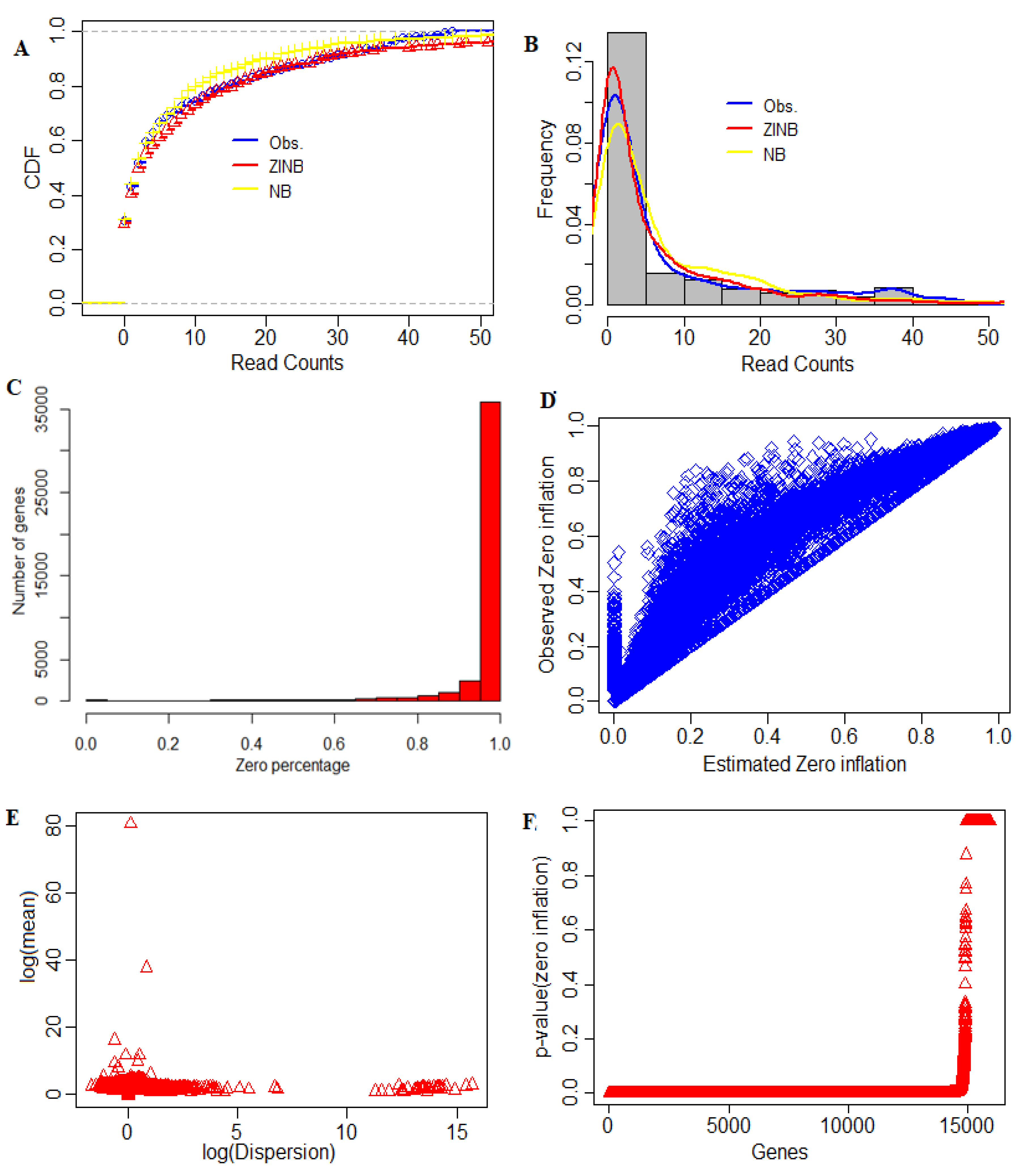
After the count data matrix was generated, we determined the percentage of zeroes in the dataset, since we were aware that there was a higher proportion of zeros present in the scRNA-seq datasets, i.e., most of the reads marked as zeros. In other words, counting the zeroes gives an idea of the presence of dropout events present in scRNA-seq data. The percentages of zeros present in each of 42,406 transcripts, as well as the fitting of the models to the data, are shown in Figure 2. Out of 42,406 transcripts, almost 35,000 had zeros over all the cells (Figure 2C). There were only fewer genes with fewer zeros across some cells (Figure 2C). Figure 2D shows the relation between observed zero proportions and estimated zero-inflation from the ZINB model. It was found that the observed zero proportions were more significant than the estimated zero-inflation parameter for each transcript. This is due to the fact that the observed zero proportions in scRNA-seq data were a mixture of the dropout zeros (i.e., zero-inflation parameter) estimated through the Dirac’s delta function and true zeros from the estimated NB model. Further, results from the statistical test of zero-inflation are shown in Figure 2F. It was found that the zero-inflation p-values for most of the genes were statistically significant (Figure 2F). This observation validated that scRNA-seq data was indeed zero-inflated due to the presence of dropout events or other experimental artifacts.
4.6. Distribution of Cell Sequencing Depths
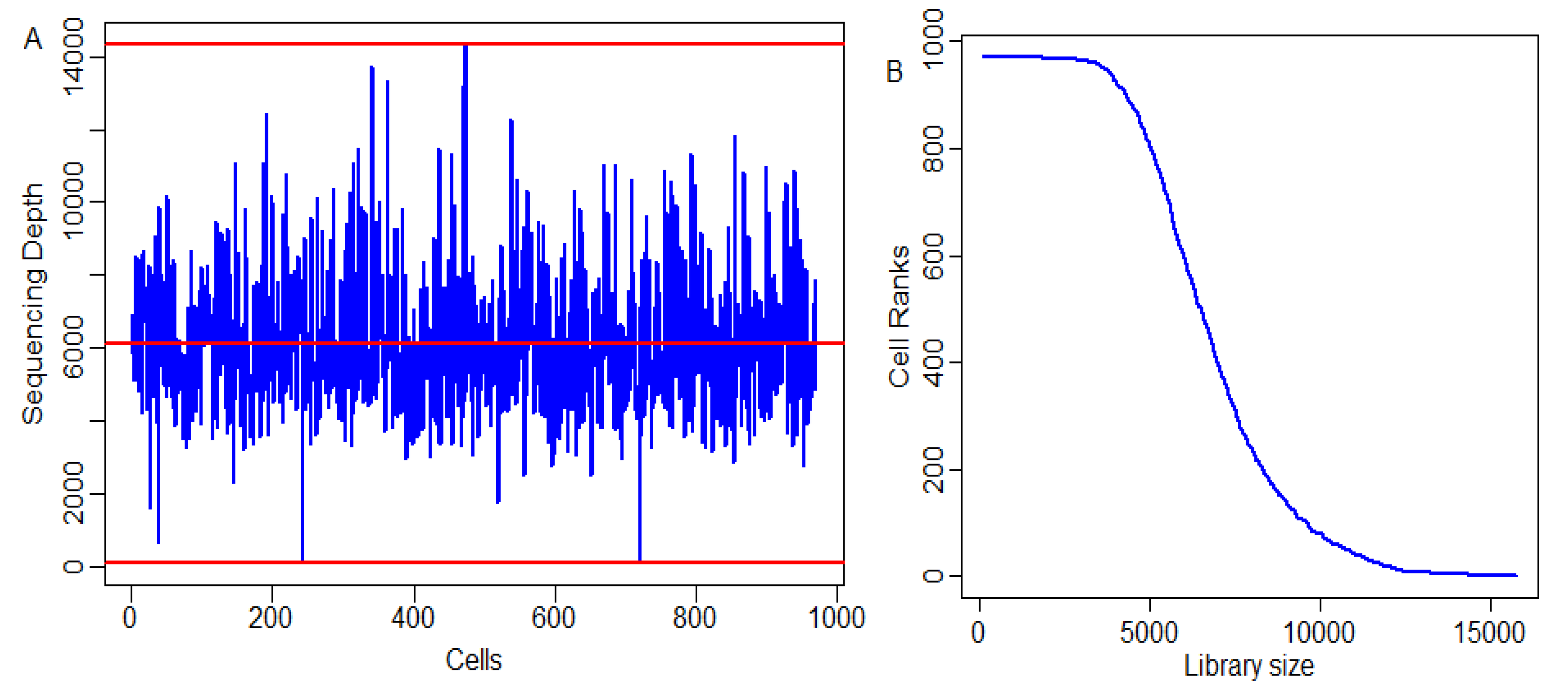
With an increase in the heterogeneity of a biological sample, a larger sample size is needed to identify and define the cell population. Determining the sequencing depth at which the majority of human transcripts are expressed in a cell and which has sufficient coverage. This has always been a debatable topic. One study showed that estimated expression levels from one million reads per cell might be adequate [49], while another study stated that a shallow sequencing depth of only 20,000 reads per cell was also sufficient [50]. Therefore, it is pertinent to study the distribution library sizes of cells in scRNA-seq data. The distribution of cell library sizes over the cells and their ranks are shown in Figure 3. The graph indicates that, out of the 972 cells, about 60% of them had a library size greater than the mean library size of 6000 (Figure 3A). Further, there existed a sigmoid-type relation among the library sizes and ranks of the cells, as depicted by the s-shaped curve (Figure 3B).
4.7. Clustering Analysis
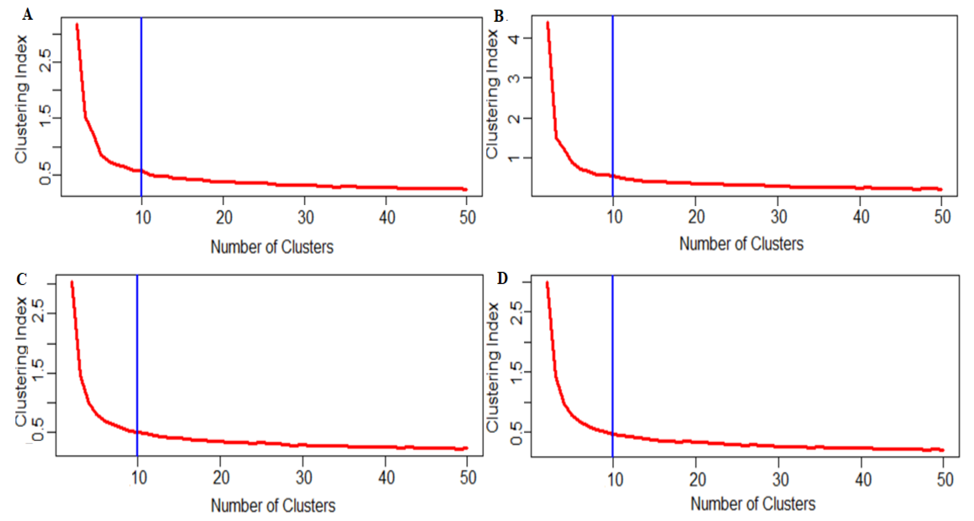
The most popular downstream analysis for scRNA-seq data is clustering, which is usually practiced to identify the cell types that exist among the cell population. However, this study remains subjective in deciding the optimum number of cell clusters that the cells present in scRNA-seq data can be divided. Here, we discussed an algorithm to determine the optimum number of cell clusters. We set the values of k as 2, 3, 4,… 50 and computed the clustering index for each k. The distribution of clustering indices over different cell cluster numbers is shown in Figure 4. Here, for lower k, we observed a higher clustering index value and this value gradually decreased with the increase in cell cluster numbers. We observed the point of inflection for this plot at k = 10 (Figure 4A). The inflection point is the point where the curve changes its direction and becomes parallel to the x-axis. In other words, the 972 cells present in the Adenocarcinoma scRNA-seq data were optimally clustered into 10 cell clusters (Figure 4A). Further, the optimal number of clusters depends on the total number of cells and the clustering index value.
4.8. Study the Effect of Zero’s Reduction on the Determination of Optimum Cell Clusters
Single-cell experiments are often performed on mixtures of multiple cell types with increased heterogeneity [53]. All genes can be analyzed, but we may add noise by including all genes that are not expressed at an adequate level to provide a meaningful result [54]. This may hinder the analysis. We can filter genes based on the average gene expression level and select genes that are unusually variable across cells.
4.9. Case 1: No Reduction
We sought to test the effect of the missing values or the zeroes on the optimal number of cell clusters. For this analysis, the dataset was reduced at various levels depending on the percentage of zeroes in the dataset. We used the complete dataset with all genes included and no reduction of any sort for this case, to determine the optimum cell clusters. The results for this entire data case are shown in Figure 4A. Here, the different number of cell clusters was plotted against their corresponding computed cluster indices. It was observed that the curve flattened at the point x = 10, which means the point of inflection for this curve was 10. So, we can say that, for the no-reduction case, the cells present in the data were optimally divided into 10 cell clusters. These observed cell clusters could be mapped to different cell types. In other words, with all 42,406 genes included in the scRNA-seq data, the 972 cells were clustered into 10 cell clusters.
4.10. Case 2: Reduction in the Number of Genes when many Cells have Zero Counts
In the second case, we reduced the number of genes based on the number of zeroes present, to find an optimal number of cell clusters. It was achieved by data reduction, whereby a certain percentage of genes whose expressions were ‘0’ in a specific percentage of cells were deleted. To be more precise, in this setting, we deleted the genes which had zero expressions in 80% cells and tried to determine the optimum number of cell clusters. This reduction process retained count expression data for 2415 genes over 972 cells. These data were used to determine the optimum number of cell clusters. The results are shown in Figure 4B. For this case, we found that the curve flattened at point 10 (i.e., point of inflection), which means the 972 cells were clustered into 10 cell clusters. In other words, the optimum number of cell clusters was 10 for 80% gene reduction. Here, we can say that gene reduction had no effect on the optimum number of cell clusters determination. This claim was further validated with other reduction scenarios and the results are shown in Table 2. Similarly, we reduced the number of genes based on 60%, 50% and 30% reduction to study the effect of gene reduction on clustering and optimal cell clusters. For a 60% reduction (i.e., number of genes reduced to 1201), the optimum cell cluster number was 10 (Table 2, Figure 4B). Similarly, for the 60% reduction case (number of genes = 1201), 50% reduction case (number of genes = 879) and 30% reduction (number of genes reduced to 454), the number of optimum cell clusters number was observed to be 10 (Table 2, Figure 4C,D, Supplementary Figure S14). From the above observations, it can be inferred that gene reduction did not affect the clustering of genes and the optimal number of clusters remained the same for all reductions. This implies that the zero counts in the data did not affect the optimal number of cell cluster determination.
4.11. Differential Expression Analysis
At the preliminary stage, we removed the cells whose library size was less than 1800 and further removed the genes which had non-zero expressions in ≤5 cells. Through this process, we selected the complete dataset having expression counts of 42,406 genes over 972 cells for further analyses. Prior to DE testing, we used the NB and ZINB models to study their suitability for fitting scRNA-seq data. The results are shown in Figure 2. The results indicate that, for fitting over-dispersed and zero-inflated datasets such as scRNA-seq, the ZINB model provided better results than the NB model (Figure 2A,B). This implies better suitability of the ZINB model for modeling the scRNA-seq count data, as well as better estimates of the parameters than the NB model. The reason may be attributed to the fact that the NB model accommodates excess zeros by underestimating the mean and overestimating the dispersion parameters [16, 51]. This phenomenon jeopardizes the statistical power of NB-based RNA-seq DE tools on discovering DE genes in the presence of zero-inflation when applied to scRNA-seq data [16].
DE testing is a well-documented problem that originates from bulk gene expression analysis [55]. Here, we compared the two methods, i.e., DESeq2 and DEsingle, which are based on two different models to identify the DE genes. At a 1% level of significance, DEsingle identified 634 genes and DESeq2 detected 79 genes with only 25 genes common between them. At a 0.1% level of significance, 401 genes were detected by DEsingle, while 75 were detected by DESeq2, with only 22 common genes detected by both methods. The results of this analysis are summarized in Table 3. Further, the list of the top 500 DE genes for the Adenocarcinoma cell lines is given in Supplementary Table S1.
From the above table, it can be concluded that NB model-based tools are not efficient in handling zero-inflated datasets such as the scRNA-seq. So, methods specific to the scRNA-seq need to be used. To substantiate our findings, we conducted a sensitivity analysis through ROC curves.
4.12. Evaluating Performance
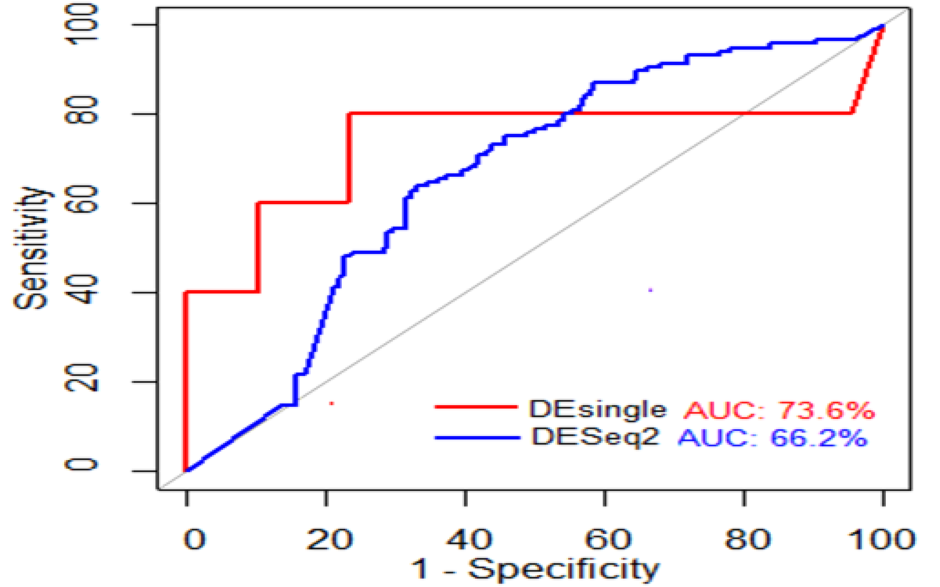
We evaluated the performances of the two DE analysis methods on these Adenocarcinoma scRNA-seq data and the results are shown in Figure 5. In other words, the ROC and AUROC of the two methods, i.e., DESeq2 and DEsingle, are shown in Figure 5.
The AUROCs for DEsingle and DESeq2 were found to be 76.2% and 66.6%, respectively (Figure 5). It is observed that DEsingle has a higher AUROC value than DESeq2 (Figure 5). This indicates that DEsingle performed better than DESeq2 on these Adenocarcinoma scRNA-seq data. This is because the ZINB model implemented in DEsingle provides better estimates of mean and dispersion than the NB model [16]. Thus, it offers better suitability of the ZINB for modeling the zero-inflated and over-dispersed scRNA-seq count data (Figure 2A,B). Further, the poor performance of DESeq2 can be attributed to the fact that the NB model accommodated excess zeros in scRNA-seq data by underestimating the mean and overestimating the dispersion, which further jeopardizes the statistical power to detect DE genes [51].
5. Conclusions
Here, we provide a comprehensive step-by-step guide for the analysis of raw scRNA-seq data. Since the noise of scRNA-seq data is high, it is crucial to use appropriate methods to overcome noises in scRNA-seq data. Quality control helps in excluding low-quality cells to avoid involving artifacts in data interpretation. The count data generated after pre-processing was zero-inflated. We observed that the number of zeroes in a dataset did not affect our clustering or cell type detection. In other words, our statistical results indicate that the zero-inflation had no or minimal role in clustering. We also provide an insight into the comparative analysis for two DE analysis tools based on the ZINB and NB models. The results indicate that the existing DE tools designed for the RNA-seq data are not capable of distinguishing the two types of zeros. Further, the sensitivity analysis-based findings suggest that bulk RNA-seq DE methods did not provide an accurate and efficient way to analyze zero-inflated scRNA-seq data.
Although many methods have been specially designed to analyze the scRNA-seq data, new techniques that can effectively handle the technical noise and expression variability of cells are still required. The new bioinformatics approaches would significantly enhance biological and clinical research and provide deep insights into the gene expression heterogeneity and cell dynamics. The approach of determining the optimum number of cell clusters is graphical, which is qualitative. Hence, a statistically sound approach needs to be developed, where the number of cell clusters is determined based on statistical significance values. To study the effect of zero-inflation on the performance on DE analysis approaches, more comprehensive computational studies need to be designed. Since there are no pre-existing clusters (such as cases and controls), selecting the optimal number of clusters may have an effect on significant gene signatures that we plan to study somewhere else.
Supplementary Materials
The following supporting information can be downloaded at: https://0-www-mdpi-com.brum.beds.ac.uk/article/10.3390/biomedinformatics2010003/s1, Figure S1: Glimpse of the Fastq file. Figure S2: Basic summary statistics of raw sequence data (fastq file). Figure S3: Per base sequence quality plot (depicting the quality of the reads in the fastq file). Figure S4: Distribution of per sequence quality scores. Figure S5: Distribution of per base sequence content. Figure S6: Distribution of per sequence GC content. Figure S7: Distribution of per base N content. Figure S8: Sequence length distribution plot. Figure S9: Sequence duplication levels plot. Figure S10: Chart of the overrepresented sequences. Figure S11: Distribution of percentage of Adapter content. Figure S12: Part of the whitelist file. Figure S13: Glimpse of resulting count matrix. Figure S14: Number of optimal clusters 60% for reduction in genes. Document S1: Linux commands for various analyses. Document S2: Data normalization. Table S1: List of top 500 differentially expressed genes.
Author Contributions
S.D. conceived and designed the study; S.D. and A.M. developed the methodologies; S.D. and A.M. contributed the R-codes and Linux codes; S.D. and A.M. contributed materials; A.M. and S.D. drafted the manuscript; S.D. and S.N.R. corrected the manuscript; S.N.R. acquired the funding. All authors have read and agreed to the published version of the manuscript.
Funding
This study was supported by Netaji Subhas-ICAR International Fellowship, OM No. 18(02)/2016-EQR/Edn. (S.D.) of Indian Council of Agricultural Research (ICAR), New Delhi, India. It was also partly supported by Wendell Cherry Chair (S.N.R.) in Clinical Trial Research, University of Louisville, USA., and multiple National Institutes of Health (NIH) grants (5P20GM113226, PI: McClain; 1P42ES023716, PI: Srivastava; 5P30GM127607-02, PI: Jones; 1P20GM125504-01, PI: Lamont; 2U54HL120163, PI: Bhatnagar/Robertson; 1P20GM135004, PI: Yan; 1R35ES0238373-01, PI: Cave; 1R01ES029846, PI: Bhatnagar; 1R01ES027778-01A1, PI: States) and Kentucky Council on Postsecondary Education grant (PON2 415 1900002934, PI: Chesney). The content is solely the responsibility of the authors and does not necessarily represent the views of NIH or ICAR.
Institutional Review Board Statement
Not applicable.
Informed Consent Statement
Not applicable.
Data Availability Statement
All the datasets used in this study are publicly available at the NCBI GEO database.
Acknowledgments
Authors duly acknowledge the help and support obtained from Education Division, ICAR, New Delhi, India and ICAR-Indian Agricultural Statistics Research Institute, New Delhi, India. Authors are extremely thankful to anonymous reviewers for their thorough suggestions and critical comments for improving the manuscript.
Conflicts of Interest
The authors declare no conflict of interest.
References
- Vallejos, C.A.; Richardson, S.; Marioni, J.C. Beyond comparisons of means: Understanding changes in gene expression at the single-cell level. Genome Biol. 2016, 17, 1. [Google Scholar] [CrossRef] [Green Version]
- Hwang, B.; Lee, J.H.; Bang, D. Single-cell RNA sequencing technologies and bioinformatics pipelines. Exp. Mol. Med. 2018, 50, 96. [Google Scholar] [CrossRef] [PubMed] [Green Version]
- Lavin, Y.; Kobayashi, S.; Leader, A.; Amir, E.-A.D.; Elefant, N.; Bigenwald, C.; Remark, R.; Sweeney, R.; Becker, C.D.; Levine, J.H.; et al. Innate Immune Landscape in Early Lung Adenocarcinoma by Paired Single-Cell Analyses. Cell 2017, 169, 750–765.e17. [Google Scholar] [CrossRef] [PubMed] [Green Version]
- Tang, F.; Barbacioru, C.; Wang, Y.; Nordman, E.; Lee, C.; Xu, N.; Wang, X.; Bodeau, J.; Tuch, B.B.; Siddiqui, A.; et al. mRNA-Seq whole-transcriptome analysis of a single cell. Nat. Methods 2009, 6, 377–382. [Google Scholar] [CrossRef]
- Scialdone, A.; Natarajan, K.N.; Saraiva, L.; Proserpio, V.; Teichmann, S.; Stegle, O.; Marioni, J.C.; Buettner, F. Computational assignment of cell-cycle stage from single-cell transcriptome data. Methods 2015, 85, 54–61. [Google Scholar] [CrossRef] [PubMed]
- Picelli, S.; Bjorklund, Å.K.; Faridani, O.; Sagasser, S.; Winberg, G.; Sandberg, R. Smart-seq2 for sensitive full-length transcriptome profiling in single cells. Nat. Methods 2013, 10, 1096–1098. [Google Scholar] [CrossRef] [PubMed]
- Brink, S.C.V.D.; Sage, F.; Vértesy, Á.; Spanjaard, B.; Peterson-Maduro, J.; Baron, C.; Robin, C.; Van Oudenaarden, A. Single-cell sequencing reveals dissociation-induced gene expression in tissue subpopulations. Nat. Methods 2017, 14, 935–936. [Google Scholar] [CrossRef] [PubMed]
- Hashimshony, T.; Senderovich, N.; Avital, G.; Klochendler, A.; de Leeuw, Y.; Anavy, L.; Gennert, D.; Li, S.; Livak, K.J.; Rozenblatt-Rosen, O.; et al. CEL-Seq2: Sensitive highly-multiplexed single-cell RNA-Seq. Genome Biol. 2016, 17, 1–7. [Google Scholar] [CrossRef] [Green Version]
- Macosko, E.Z.; Basu, A.; Satija, R.; Nemesh, J.; Shekhar, K.; Goldman, M.; Tirosh, I.; Bialas, A.R.; Kamitaki, N.; Martersteck, E.M.; et al. Highly Parallel Genome-wide Expression Profiling of Individual Cells Using Nanoliter Droplets. Cell 2015, 161, 1202–1214. [Google Scholar] [CrossRef] [PubMed] [Green Version]
- Zemmour, D.; Zilionis, R.; Kiner, E.; Klein, A.M.; Mathis, D.; Benoist, C. Single-cell gene expression reveals a landscape of regulatory T cell phenotypes shaped by the TCR. Nat. Immunol. 2018, 19, 291–301. [Google Scholar] [CrossRef] [PubMed]
- Jaitin, D.A.; Kenigsberg, E.; Keren-Shaul, H.; Elefant, N.; Paul, F.; Zaretsky, I.; Mildner, A.; Cohen, N.; Jung, S.; Tanay, A.; et al. Massively parallel single-cell RNA-seq for marker-free decomposition of tissues into cell types. Science 2014, 343, 776–779. [Google Scholar] [CrossRef] [PubMed]
- Ramsköld, D.; Luo, S.; Wang, Y.-C.; Li, R.; Deng, Q.; Faridani, O.; Daniels, G.A.; Khrebtukova, I.; Loring, J.F.; Laurent, L.; et al. Full-length mRNA-Seq from single-cell levels of RNA and individual circulating tumor cells. Nat. Biotechnol. 2012, 30, 777–782. [Google Scholar] [CrossRef] [Green Version]
- Ziegenhain, C.; Vieth, B.; Parekh, S.; Reinius, B.; Guillaumet-Adkins, A.; Smets, M.; Leonhardt, H.; Enard, W. Comparative Analysis of Single-Cell RNA Sequencing Methods. Mol. Cell 2017, 65, 631–643.e4. [Google Scholar] [CrossRef] [Green Version]
- Wang, Z.; Gerstein, M.; Snyder, M. RNA-seq: A revolutionary tool for transcriptomics. Nat. Rev. Genet. 2009, 10, 57–63. [Google Scholar] [CrossRef] [PubMed]
- Kolodziejczyk, A.; Kim, J.K.; Svensson, V.; Marioni, J.; Teichmann, S.A. The technology and biology of single-cell RNA sequencing. Mol. Cell 2015, 58, 610–620. [Google Scholar] [CrossRef] [PubMed] [Green Version]
- Das, S.; Rai, A.; Merchant, M.L.; Cave, M.C.; Rai, S.N. A Comprehensive Survey of Statistical Approaches for Differential Expression Analysis in Single-cell RNA Sequencing Studies. Genes 2021, 12, 1947. [Google Scholar] [CrossRef]
- Bacher, R.; Kendziorski, C. Design and computational analysis of single-cell RNA-sequencing experiments. Genome Biol. 2016, 17, 63. [Google Scholar] [CrossRef] [PubMed] [Green Version]
- Brennecke, P.; Anders, S.; Kim, J.K.; Kolodziejczyk, A.; Zhang, X.; Proserpio, V.; Baying, B.; Benes, V.; Teichmann, S.; Marioni, J.; et al. Accounting for technical noise in single-cell RNA-seq experiments. Nat. Methods 2013, 10, 1093–1095. [Google Scholar] [CrossRef] [PubMed]
- Blower, M.D.; Jambhekar, A.; Schwarz, D.S.; Toombs, J. Combining Different mRNA Capture Methods to Analyze the Transcriptome: Analysis of the Xenopus laevis Transcriptome. PLoS ONE 2013, 8, e77700. [Google Scholar] [CrossRef]
- Hicks, S.C.; Townes, F.W.; Teng, M.; Irizarry, R. Missing data and technical variability in single-cell RNA-sequencing experiments. Biostatistics 2018, 19, 562–578. [Google Scholar] [CrossRef]
- Haque, A.; Engel, J.; Teichmann, S.A.; Lönnberg, T. A practical guide to single-cell RNA-sequencing for biomedical research and clinical applications. Genome Med. 2017, 9, 75. [Google Scholar] [CrossRef] [PubMed]
- Qiu, P. Embracing the dropouts in single-cell RNA-seq analysis. Nat. Comm. 2020, 11, 1169. [Google Scholar] [CrossRef] [Green Version]
- Lafzi, A.; Moutinho, C.; Picelli, S.; Heyn, H. Tutorial: Guidelines for the experimental design of single-cell RNA sequencing studies. Nat. Protoc. 2018, 13, 2742–2757. [Google Scholar] [CrossRef] [PubMed] [Green Version]
- Luecken, M.D.; Theis, F.J. Current best practices in single-cell RNA-seq analysis: A tutorial. Mol. Syst. Biol. 2019, 15, e8746. [Google Scholar] [CrossRef]
- Andrews, T.S.; Kiselev, V.Y.; McCarthy, D.; Hemberg, M. Tutorial: Guidelines for the computational analysis of single-cell RNA sequencing data. Nat. Protoc. 2021, 16, 1–9. [Google Scholar] [CrossRef]
- Love, M.I.; Huber, W.; Anders, S. Moderated estimation of fold change and dispersion for RNA-seq data with DESeq2. Genome Biol. 2014, 15, 550. [Google Scholar] [CrossRef] [PubMed] [Green Version]
- Miao, Z.; Deng, K.; Wang, X.; Zhang, X. DEsingle for detecting three types of differential expression in single-cell RNA-seq data. Bioinformatics 2018, 34, 3223–3224. [Google Scholar] [CrossRef] [Green Version]
- Tian, L.; Su, S.; Dong, X.; Amann-Zalcenstein, D.; Biben, C.; Seidi, A.; Hilton, D.J.; Naik, S.H.; Ritchie, M.E. scPipe: A flexible R/Bioconductor preprocessing pipeline for single-cell RNA-sequencing data. PLoS Comput. Biol. 2018, 14, e1006361. [Google Scholar] [CrossRef]
- Tian, L.; Dong, X.; Freytag, S.; Cao, K.-A.L.; Su, S.; JalalAbadi, A.; Amann-Zalcenstein, D.; Weber, T.S.; Seidi, A.; Jabbari, J.S.; et al. Benchmarking single cell RNA-sequencing analysis pipelines using mixture control experiments. Nat. Methods 2019, 16, 479–487. [Google Scholar] [CrossRef] [PubMed]
- Cock, P.J.; Fields, C.J.; Goto, N.; Heuer, M.L.; Rice, P.M. The Sanger FASTQ file format for sequences with quality scores, and the Solexa/Illumina FASTQ variants. Nucleic Acids Res. 2010, 38, 1767–1771. [Google Scholar] [CrossRef] [PubMed] [Green Version]
- Sequence Read Archives. Available online: https://trace.ncbi.nlm.nih.gov/Traces/sra/sra.cgi?view=software (accessed on 10 November 2020).
- Leinonen, R.; Sugawara, H.; Shumway, M.; on behalf of the International Nucleotide Sequence Database Collaboration. The Sequence Read Archive. Nucleic Acids Res. 2010, 39, D19–D21. [Google Scholar] [CrossRef] [Green Version]
- Andrews, S. FastQC-A Quality Control Tool for High throughput Sequence Data. 2014. Available online: http://www.bioinformatics.babraham.ac.uk/projects/fastqc/ (accessed on 10 November 2020).
- Smith, T.; Heger, A.; Sudbery, I. UMI-tools: Modeling sequencing errors in Unique Molecular Identifiers to improve quantification accuracy. Genome Res. 2017, 27, 491–499. [Google Scholar] [CrossRef] [Green Version]
- “GRC and Collaborators”. Genome Reference Consortium. Available online: https://0-www-ncbi-nlm-nih-gov.brum.beds.ac.uk/grc/credits/ (accessed on 19 October 2020).
- Harrow, J.; Frankish, A.; Gonzalez, J.M.; Tapanari, E.; Diekhans, M.; Kokocinski, F.; Aken, B.L.; Barrell, D.; Zadissa, A.; Searle, S.; et al. GENCODE: The reference human genome annotation for The ENCODE Project. Genome Res. 2012, 22, 1760–1774. [Google Scholar] [CrossRef] [PubMed] [Green Version]
- Dobin, A.; Davis, C.A.; Schlesinger, F.; Drenkow, J.; Zaleski, C.; Jha, S.; Batut, P.; Chaisson, M.; Gingeras, T.R. Gingeras, STAR: Ultrafast universal RNA-seq aligner. Bioinformatics 2013, 29, 15–21. [Google Scholar] [CrossRef]
- Li, H.; Handsaker, B.; Wysoker, A.; Fennell, T.; Ruan, J.; Homer, N.; Marth, G.; Abecasis, G.; Durbin, R.; 1000 Genome Project Data Processing Subgroup. The Sequence Alignment/Map format and SAMtools. Bioinformatics 2009, 25, 2078–2079. [Google Scholar] [CrossRef] [Green Version]
- Liao, Y.; Smyth, G.K.; Shi, W. featureCounts: An efficient general-purpose program for assigning sequence reads to genomic features. Bioinformatics 2014, 30, 923–930. [Google Scholar] [CrossRef] [PubMed] [Green Version]
- R Core Team. R: A Language and Environment for Statistical Computing; R Foundation for Statistical Computing: Vienna, Austria, 2019. [Google Scholar]
- Hartigan, J.A.; Wong, M.A. Algorithm AS 136: A K-Means Clustering Algorithm. J. R. Stat. Soc. Ser. C (Appl. Stat.) 1979, 28, 100–108. [Google Scholar] [CrossRef]
- Ewing, B.; Hillier, L.; Wendl, M.C.; Green, P. Base-calling of automated sequencer traces using Phred. I. Accuracy assessment. Genome Res. 1998, 8, 175–185. [Google Scholar] [CrossRef] [PubMed] [Green Version]
- Batut, B.; Hiltemann, S.; Bagnacani, A.; Baker, D.; Bhardwaj, V.; Blank, C.; Bretaudeau, A.; Brillet-Guéguen, L.; Čech, M.; Chilton, J.; et al. 2018 Community-Driven Data Analysis Training for Biology. Cell Syst. 2018, 6, 752–758.e1. [Google Scholar] [CrossRef] [PubMed] [Green Version]
- Dobin, A.; Gingeras, T.R. Mapping RNA-seq Reads with STAR. Curr. Protoc. Bioinform. 2015, 51, 1–19. [Google Scholar] [CrossRef] [PubMed] [Green Version]
- GENOCODE. Available online: https://www.gencodegenes.org/human/stats.html (accessed on 15 November 2020).
- Robinson, M.D.; McCarthy, D.J.; Smyth, G.K. EdgeR: A Bioconductor package for differential expression analysis of digital gene expression data. Bioinformatics 2010, 26, 139–140. [Google Scholar] [CrossRef] [PubMed] [Green Version]
- Hardcastle, T.; Kelly, K. BaySeq: Empirical Bayesian Methods for Identifying Differential Expression in Sequence Count Data. BMC Bioinform. 2010, 11, 422. [Google Scholar] [CrossRef] [PubMed] [Green Version]
- Li, W.V.; Li, J.J. An accurate and robust imputation method scImpute for single-cell RNA-seq data. Nat Commun. 2018, 9, 997. [Google Scholar] [CrossRef] [PubMed] [Green Version]
- Lun, A.T.L.; Bach, K.; Marioni, J.C. Pooling Across Cells to Normalize Single-Cell Rna Sequencing Data with Many Zero Counts. Genome Biol. 2016, 17, 75. [Google Scholar] [CrossRef] [PubMed]
- Žurauskienė, J.; Yau, C. PcaReduce: Hierarchical clustering of single-cell transcriptional profiles. BMC Bioinform. 2016, 17, 140. [Google Scholar] [CrossRef] [PubMed] [Green Version]
- Das, S.; Rai, S.N. SwarnSeq: An improved statistical approach for differential expression analysis of single-cell RNA-seq data. Genomics 2021, 113, 1308–1324. [Google Scholar] [CrossRef]
- Das, S.; Rai, S.N. Statistical methods for analysis of single-cell RNA-sequencing data. MethodsX 2021, 8, 101580. [Google Scholar] [CrossRef]
- Shalek, A.K.; Satija, R.; Shuga, J.; Trombetta, J.J.; Gennert, D.; Lu, D.; Chen, P.; Gertner, R.S.; Gaublomme, J.T.; Yosef, N.; et al. Single-cell RNA-seq reveals dynamic paracrine control of cellular variation. Nature 2014, 510, 363–369. [Google Scholar] [CrossRef] [Green Version]
- Pierson, E.; Yau, C. Zifa: Dimensionality reduction for zero-inflated single-cell gene expression analysis. Genome Biol. 2015, 16, 241. [Google Scholar] [CrossRef] [Green Version]
- Scholtens, D.; von Heydebreck, A. Analysis of Differential Gene Expression Studies. In Bioinformatics and Computational Biology Solutions Using R and Bioconductor; Gentleman, R., Carey, V.J., Huber, W., Irizarry, R.A., Dudoit, S., Eds.; Statistics for Biology and Health; Springer: New York, NY, USA, 2005. [Google Scholar] [CrossRef]
Figure 1.
Outlines of the workflow for various steps in scRNA-seq data analysis. (A) Key steps involved in a typical single-cell RNA-seq experiment starting from the sample preparation by the isolation and lysis of single cells up to the data analysis. (B) Data preprocessing steps beginning from the .fastq files up to the generation of count matrix and the tools required at each stage. (C) Significant data analysis steps with the input count data matrix undertaken in the scRNA-seq study.

Figure 2.
Data structure model, distributions and estimated parameters. (A) Different cumulative distribution function (CDF) fitted to the single adenocarcinoma cells RNA-seq data. The x-axis corresponds to the cumulative densities and the y-axis represents the read counts. The red color corresponds to the observed CDF, the pink color to NB and the blue color to ZINB. (B) Fitting of count data models to the given adenocarcinoma single cells RNA-seq data. In this plot, the x-axis represents the scRNA-seq read counts and the y-axis represents the densities. The red color corresponds to the observed density, the pink color to NB density and the blue color to ZINB density. (C) Distribution of zeroes. The x-axis is the number of genes and the y-axis shows the percentage of zeroes. (D) Plotting of observed zero proportions vs. estimated zero-inflation. The x-axis represents the estimated zero-inflation and the y-axis represents the observed zero proportion. Here, the plot shows that the observed zero proportions are greater than the estimated zero-inflation. (E) Relation between mean and dispersion. The log(mean) is shown on the y-axis vs. log(dispersion) on the x-axis. (F) The plot shows zero-inflation in data. The y-axis corresponds to the p-value and the x-axis represents the genes.

Figure 3.
Distribution of cell sizes for Adenocarcinoma scRNA-seq data. (A) Distribution of library sizes across the total number of cells. (B) Plot for cell ranks vs. cell sizes—distribution of cell library sizes over the cell ranks. Here, the y-axis represents the cells’ rank and the x-axis represents the sequencing depth.

Figure 4.
Effects of zero reductions on the determination of an optimum number of cell clusters. The figures are shown for (A) no reduction, (B) 80% reduction, (C) 50% reduction and (D) 30% reduction. The y-axis represents the values of clustering indices and the x-axis represents the values of optimum cell clusters. The blue line indicates the value of the optimum number of cell clusters in which the cells in the data can be clustered. For (A), we observe the optimal number of clusters is approximately 10 for the 972 cells with all genes included. (B) 80% reduction (80% reduction of zeros with 2415 reduced genes): the number of cell clusters was found to be 10.. (C) 50% reduction (50% reduction of zeros with 879 reduced genes): the number of cell clusters was found to be 10. (D) 30% reduction (30% reduction of zeros and with 454 genes): the number of cell clusters was found to be 10.

Figure 5.
Comparative analysis of DEsingle and DESeq2 in terms of AUROC. The figure shows the ROC curves of the two DE analysis methods, DESeq2 and DEsingle. The red color indicates the DEsingle and the blue color represents DESeq2. DEsingle has better performance in terms of AUC value as compared to DESeq2.


Table 1.
List of the tools used in this study.
| Name | Version | Description | Reference |
|---|---|---|---|
| FastQC | v0.11.9 | FastQ Quality Check | [33] |
| UMI-tools | 1.0.0 | Tools for handling Unique Molecular Identifiers | [34] |
| Human genome | Grch38/hg 38 | Human genome reference file | [35] |
| GTF | Release 35 | Gene Transfer Format | [36] |
| STAR | 2.7 | Spliced Transcripts Alignment to a Reference | [37] |
| SAM tools | 1.4 | SAMtools software package | [38] |
| Subread package | 2.0.1 | The package used by SAMtools | [39] |
| Stats R package | 3.6.1 | Package for k-means clustering | [40,41] |
| DESeq2 | 1.28.1 | DE analysis tool for RNA-seq | [26] |
| DEsingle | 1.8.2 | DE analysis tool for scRNA-seq | [27] |
Table 2.
Lists the optimal number of clusters and the number of genes in each reduction.
| Case Type | Percentage Reduction | No. of Optimal Clusters | No. of Genes |
|---|---|---|---|
| Case 1 | No reduction | 10 | 42,406 |
| Case 2 | 80% | 10 | 2415 |
| Case 2 | 60% | 10 | 1201 |
| Case 2 | 50% | 10 | 879 |
| Case 2 | 30% | 10 | 454 |
Table 3.
Summary of results from a comparative analysis of DEsingle and DESeq2 using case I clustering method.
Table 3.
Summary of results from a comparative analysis of DEsingle and DESeq2 using case I clustering method.
| Level of Significance | DEsingle Genes | DESeq2 Genes | Common Genes |
|---|---|---|---|
| 1% | 634 | 79 | 25 |
| 0.1% | 401 | 75 | 22 |
Publisher’s Note: MDPI stays neutral with regard to jurisdictional claims in published maps and institutional affiliations. |
© 2021 by the authors. Licensee MDPI, Basel, Switzerland. This article is an open access article distributed under the terms and conditions of the Creative Commons Attribution (CC BY) license (https://creativecommons.org/licenses/by/4.0/).
Share and Cite
MDPI and ACS Style
Malhotra, A.; Das, S.; Rai, S.N. Analysis of Single-Cell RNA-Sequencing Data: A Step-by-Step Guide. BioMedInformatics 2022, 2, 43-61. https://0-doi-org.brum.beds.ac.uk/10.3390/biomedinformatics2010003
AMA Style
Malhotra A, Das S, Rai SN. Analysis of Single-Cell RNA-Sequencing Data: A Step-by-Step Guide. BioMedInformatics. 2022; 2(1):43-61. https://0-doi-org.brum.beds.ac.uk/10.3390/biomedinformatics2010003
Chicago/Turabian StyleMalhotra, Aanchal, Samarendra Das, and Shesh N. Rai. 2022. "Analysis of Single-Cell RNA-Sequencing Data: A Step-by-Step Guide" BioMedInformatics 2, no. 1: 43-61. https://0-doi-org.brum.beds.ac.uk/10.3390/biomedinformatics2010003