Article

Projection of High-Dimensional Genome-Wide Expression on SOM Transcriptome Landscapes

by
Maria Nikoghosyan
1,2,†,
Henry Loeffler-Wirth
3,†,
Suren Davidavyan
1,2,
Hans Binder
2,4 and
Arsen Arakelyan
1,2,*
1
Bioinformatics Group, Institute of Molecular Biology, National Academy of Science of the Republic of Armenia, Yerevan 0014, Armenia
2
Department of Bioengineering, Bioinformatics and Molecular Biology, Russian-Armenian University, Yerevan 0051, Armenia
3
Interdisciplinary Centre for Bioinformatics, Leipzig University, 04107 Leipzig, Germany
4
Armenian Bioinformatics Institute, Yerevan 0051, Armenia
*
Author to whom correspondence should be addressed.
These authors contributed equally to this work.
Submission received: 2 December 2021 / Revised: 17 December 2021 / Accepted: 22 December 2021 / Published: 27 December 2021

Abstract

:
The self-organizing maps portraying has been proven to be a powerful approach for analysis of transcriptomic, genomic, epigenetic, single-cell, and pathway-level data as well as for “multi-omic” integrative analyses. However, the SOM method has a major disadvantage: it requires the retraining of the entire dataset once a new sample is added, which can be resource- and time-demanding. It also shifts the gene landscape, thus complicating the interpretation and comparison of results. To overcome this issue, we have developed two approaches of transfer learning that allow for extending SOM space with new samples, meanwhile preserving its intrinsic structure. The extension SOM (exSOM) approach is based on adding secondary data to the existing SOM space by “meta-gene adaptation”, while supervised SOM portrayal (supSOM) adds support vector machine regression model on top of the original SOM algorithm to “predict” the portrait of a new sample. Both methods have been shown to accurately combine existing and new data. With simulated data, exSOM outperforms supSOM for accuracy, while supSOM significantly reduces the computing time and outperforms exSOM for this parameter. Analysis of real datasets demonstrated the validity of the projection methods with independent datasets mapped on existing SOM space. Moreover, both methods well handle the projection of samples with new characteristics that were not present in training datasets.

1. Introduction

The high-dimensional low sample size nature of modern -omics datasets necessitates application of dimensionality reduction and clustering approaches for their efficient analysis. The self-organizing maps (SOM) portrayal method implemented in the oposSOM package [1] has been proven to be a powerful approach for analysis of differential expression [2], molecular subtyping [3], and sample stratification [4]. SOM clusters gene expression profiles (vectors of gene expression values across samples) into miniclusters called meta-genes and projects high-dimensional data into two-dimensional maps. SOM clustering coupled with extensive downstream functional analyses allows for comprehensive annotation of transcriptome landscape, identification of co-expressed gene clusters, and linking them to biological processes using curated sets of genes with known functional background [5]. In contrast to other clustering and dimension reduction approaches, the SOM method allows for feature extraction and offers a mechanistic interpretation of underlying biological mechanisms in terms of molecular “portraits”, and spot modules of co-overexpressed genes [6]. Moreover, the SOM method was extended to the analysis of genomic [7], epigenetic [8], single-cell [9], and pathway-level [10] data as well as for “multi-omic” integrative analyses [11].
However, the SOM method has a major disadvantage: it requires the retraining of the entire dataset once a new sample is added. In the case of few samples in the new dataset, this is a valid approach [12,13], but once the number of samples is large, or individual samples are being added consecutively, it could be time- and computing resource-consuming. Moreover, retraining causes the change of gene arrangements, thus making the results hard to compare.
To address this issue, we have developed two new approaches that allow for extending SOM space with new samples, meanwhile preserving its intrinsic structure. The extension SOM (exSOM) approach is based on adding secondary data to the existing SOM space, while supervised SOM portrayal (supSOM) adds support vector machine regression model on top of the original SOM algorithm and allows “predicting” the portrait of a new sample. Both methods reuse information of the primary SOM for improved sampling efficiency of the secondary data and as such refers to transfer learning in SOM space. They have been shown to accurately combine existing and new data. exSOM is characterized by higher accuracy compared to supSOM, while the latter is useful when the sample size to secondary data is large, or samples are obtained sequentially.

2. Materials and Methods

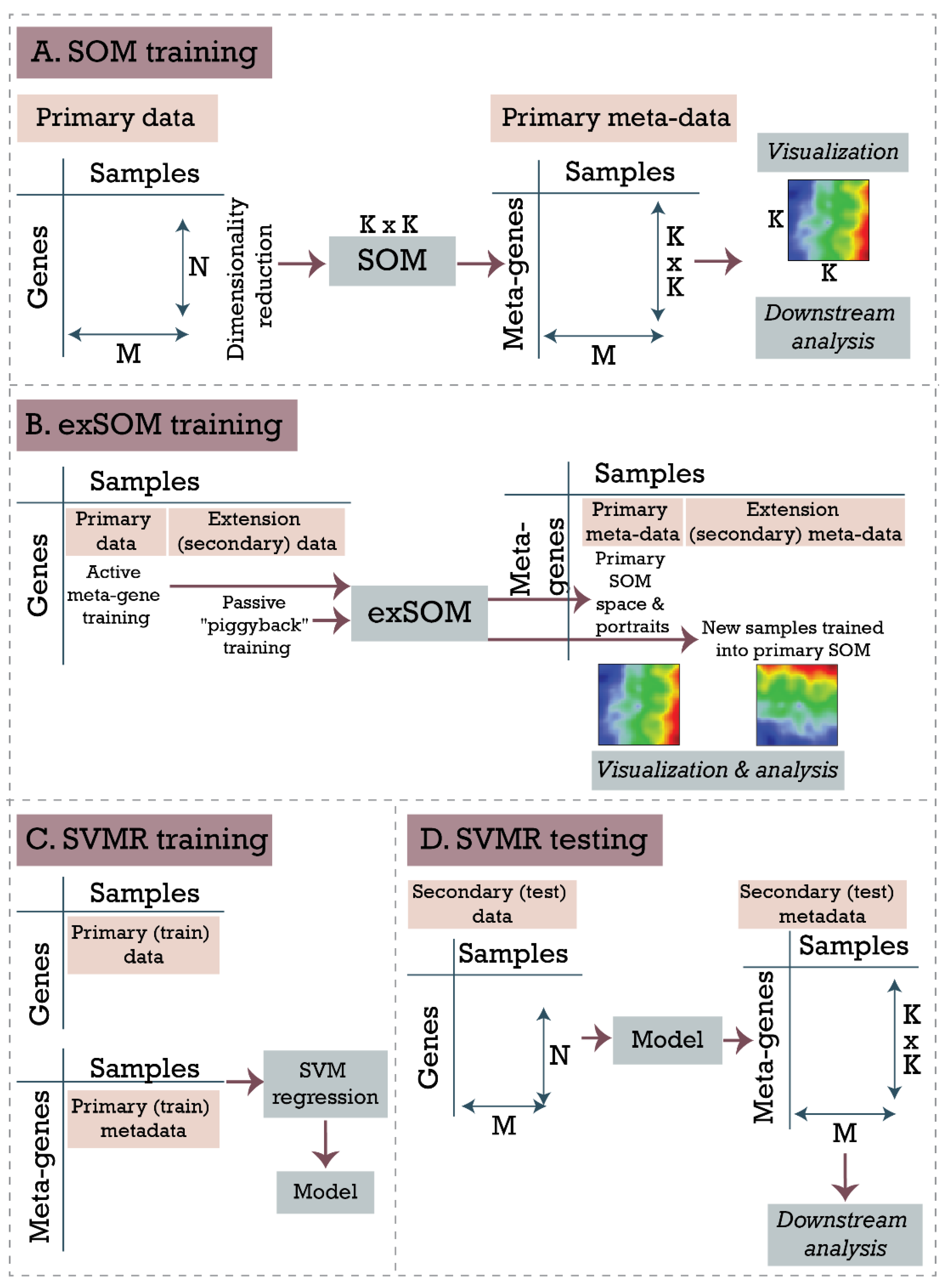
2.1. General Workflow

The general workflow of the algorithms is presented in Figure 1. In both cases, the “primary” dataset is trained with self-organizing maps (SOM), followed by clustering and downstream analysis [1] (Figure 1A). In exSOM, “secondary” data is added to the existing SOM space by passive training (Figure 1B). For supSOM, the support vector machine regression model (SVMR) is trained that maps input expression dataset to SOM “portraits” generated from “primary” data. Finally, a “secondary” dataset is supplied to the model for projection into the SOM space (Figure 1C). Below, the details of each algorithm are addressed in detail.

2.2. Self-Organizing Map (SOM) Training and Downstream Functional Analysis

The SOM algorithm realizes three main analysis tasks (Figure 1A): (1) dimension reduction of the single gene expression profiles into a reduced set of meta-gene profiles, (2) thereby clustering of similar gene profiles, and (3) multidimensional scaling represented by the mapping of each gene into the two-dimensional SOM grid. We used the parallelized SOM training algorithm implemented in Bioconductor R-package “oposSOM” [1]. The method projects high-dimensional gene expression data into a two-dimensional space: N (genes) × M (samples) gene expression matrix is translated into K (meta-genes) × M (samples) matrix of reduced dimensionality [14,15]. Genes are assigned to meta-genes based on the similarity of expression profiles across the samples. Each meta-gene profile can be interpreted as the mean profile averaged over all gene profiles of the respective meta-gene cluster. During the SOM training phase, the algorithm distributes the genes over the meta-genes using the Euclidean distance between the gene and meta-gene profiles as a similarity measure. Meta-genes are arranged in a k × k = K two-dimensional grid coordinate system and colored according to their expression level for each sample, providing the so-called “expression portraits” [1]. Group-specific mean portraits are generated by averaging the portraits of all cases belonging to a given group or subtype.
In the SOM space, genes with similar profiles are located in adjacent meta-genes, which form “spot-like” areas of up- and downregulated expression meta-gene clusters on the map due to the self-organizing properties of the SOM. These spots represent clusters of co-regulated genes, termed expression modules, and their patterns are a characteristic fingerprint of each particular sample/group of samples. Lists of genes included in each of the spot modules provide a functional context of the spot and were evaluated with gene-set enrichment analysis approaches [14].

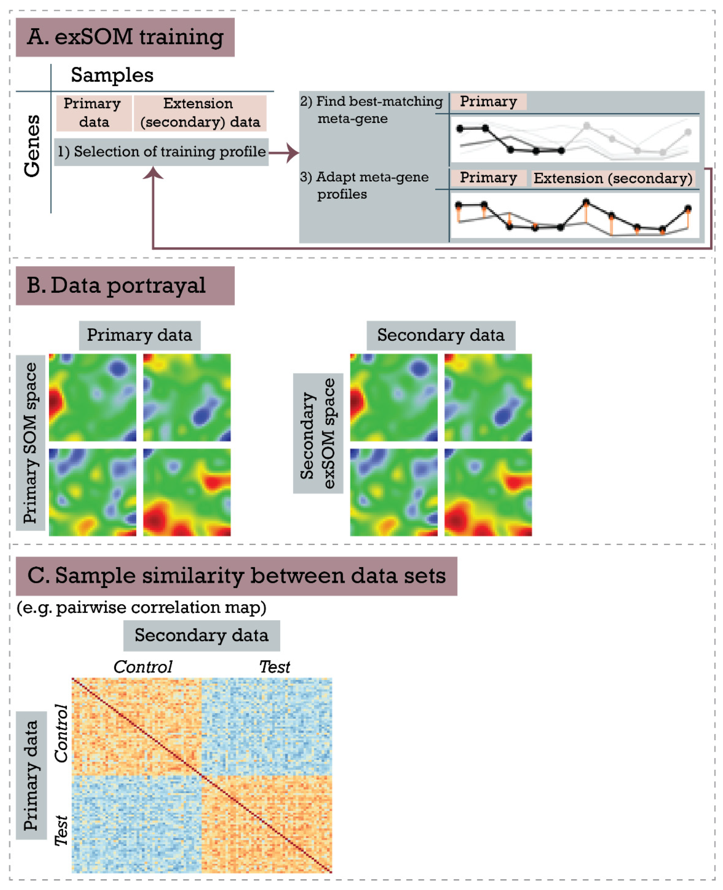
2.3. Extension SOM Training (exSOM)

The SOM extension method (exSOM) aims at adding new, secondary data (e.g., independent data on the same system obtained from follow-up studies or web repositories) to an already existing SOM space (e.g., that of the primary data portraying analysis). For this, the original SOM algorithm was adapted to realize standard meta-gene training for the samples already contained in the primary SOM training, and a passive, “piggyback” training of the meta-genes for the extension data (Figure 1B). In brief, the exSOM training algorithms comprise three steps analogous to the SOM training, which are iteratively repeated until a convergence criterion (e.g., predefined absolute number of iterations) is achieved:
  • Training profile selection: A gene profile (i.e., a vector of expression values for all samples) is selected, usually by sequential order.
  • Determination of best-matching meta-gene: The meta-gene profile, which is the most similar to the training profile, is determined using the Euclidean distance metric. Importantly, only data points corresponding to the original samples contribute to the similarity metric; data points of the extension samples are not considered in this step. This ensures that gene to meta-gene assignment is not altered by adding the extension samples when compared to the primary SOM training.
  • Meta-gene adaptation: The expression values of the meta-genes are adapted according to the Hebbian learning rule according to the original SOM training algorithm [16]. It combines the difference between the training and the meta-gene profiles with a learning rate and a neighborhood factor, both incrementally decreasing as the training proceeds. In this step, samples from the original and the extension set are considered, resulting in iteratively optimized meta-gene expression values for all samples.
This training algorithm eventually provides unchanged meta-gene values for the primary data and new, adapted meta-gene data for the secondary data, allowing for direct comparison and integrated downstream analyses.

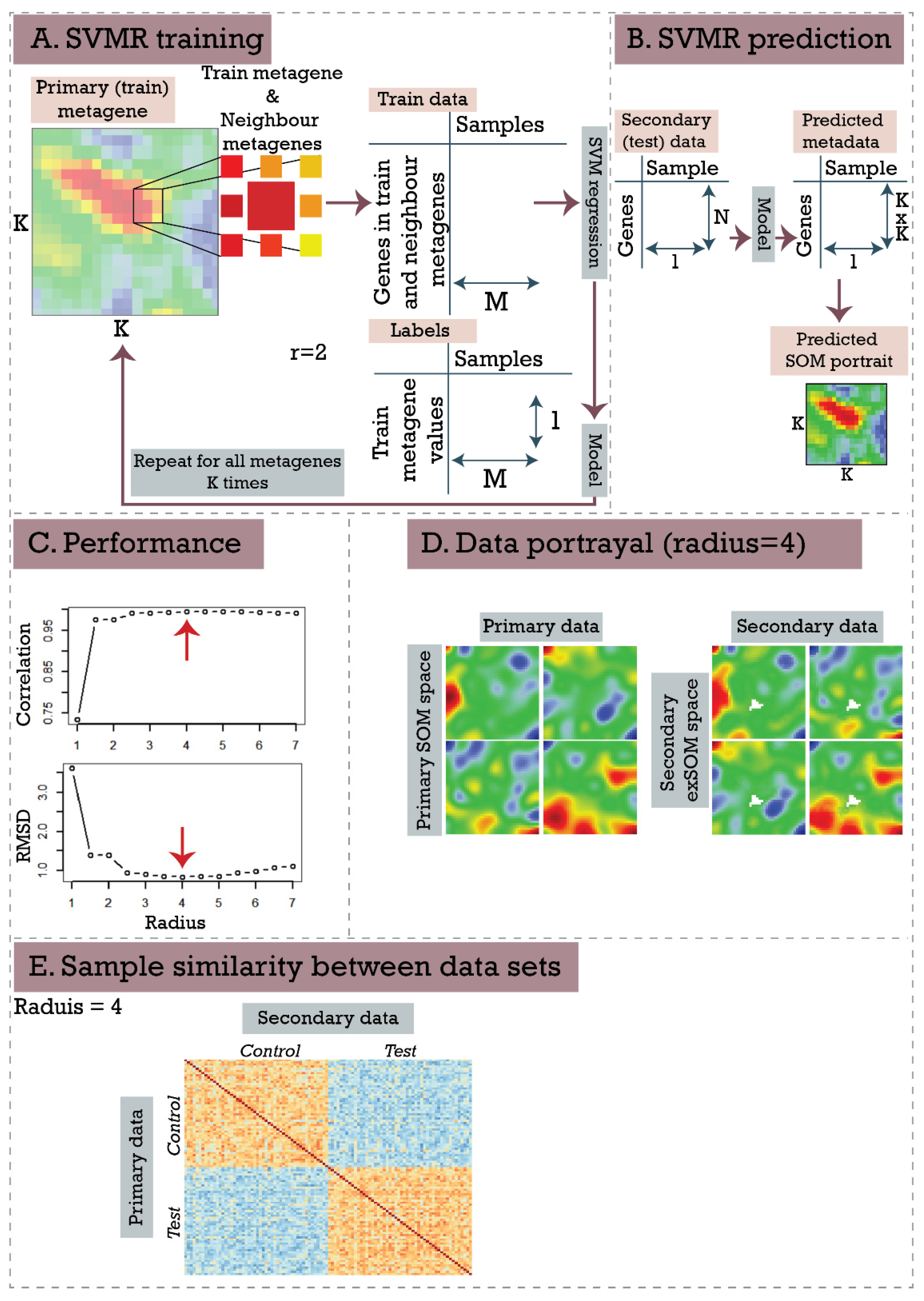
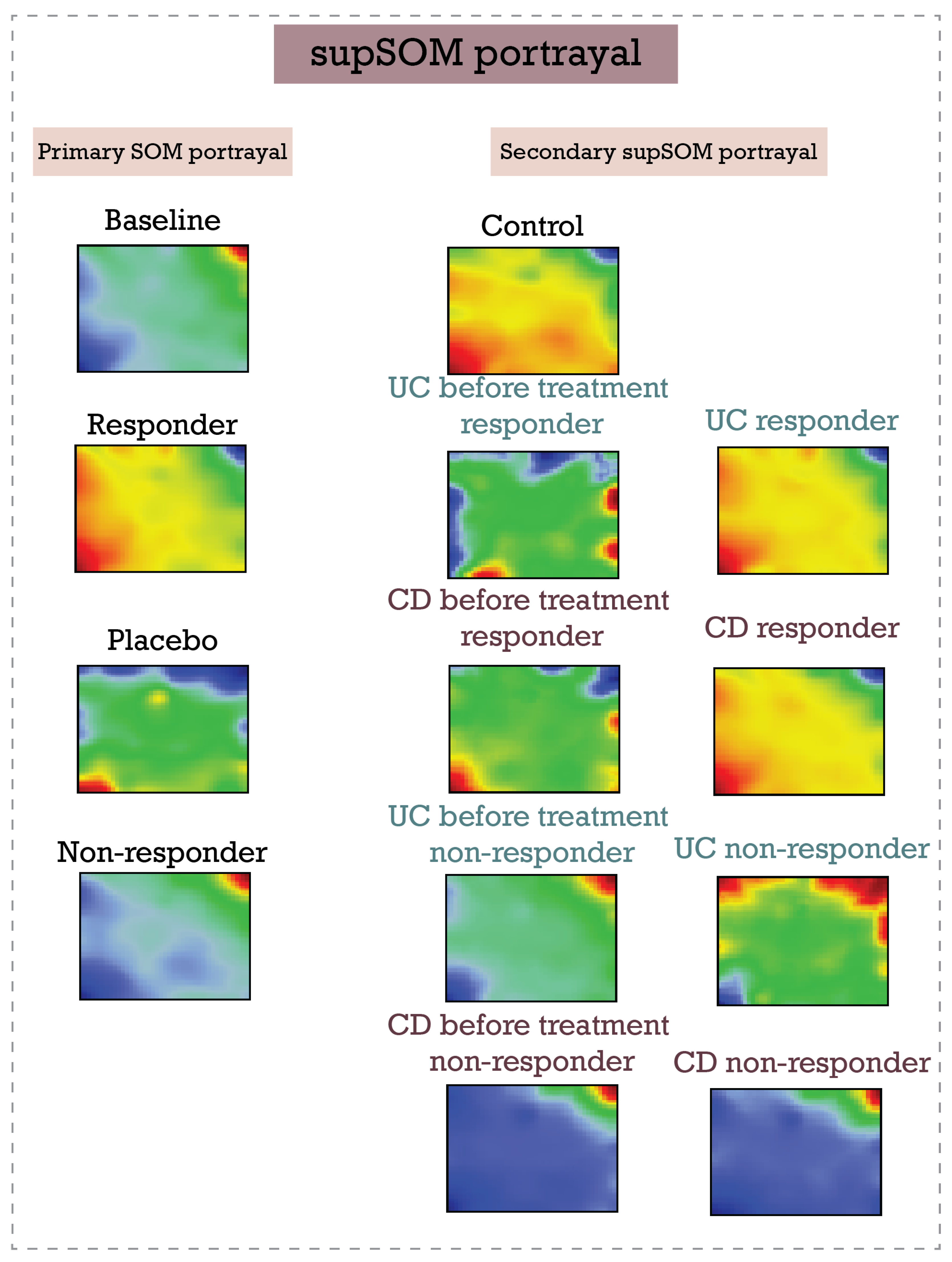
2.4. Supervised SOM Portrayal (supSOM)

Supervised SOM (supSOM) portrayal is based on support vector machine regression (SVMR) and provides an alternative approach for extending an existing SOM space. In supSOM, one SVMR model is trained for each meta-gene individually, using the genes’ expression profiles of the primary data as independent variable, and the corresponding meta-gene profile obtained from the initial SOM training as dependent variable. Thereby, only genes associated with the particular meta-gene or one of the adjacent meta-genes are considered as predictors. Once a model is trained, gene profiles in new samples can be used to predict the corresponding meta-genes (Figure 1C). We applied SVM regression model with Gaussian kernel and evaluated supSOM performance for varying neighborhood radii.

2.5. Performance Assessment with Simulated Datasets

Performance and accuracy for exSOM and supSOM were assessed based on evaluation of correlation and root-mean-square deviation (RMSD) between metadata of the extension samples (i.e., the portraits) generated by SOM as reference vs. exSOM or vs. supSOM.
For benchmarking runtime of the SOM initialization and training phases, we generated artificial expression matrices for the primary and secondary (extension) data (m1 = m2 = 50, 100, 200, 500, and 1000 arrays per class) using the “madsim” R package [17] (for parameters, see Text S1).

2.6. Use-Case Datasets

We used the supSOM and exSOM approaches to evaluate the effect of infliximab treatment on transcriptome landscapes in ulcerative colitis and Crohn’s disease (GSE23597 and GSE16879) and to study disease grade-associated transcriptome changes in breast cancer (GSE42568, GSE10810, and GSE29431), respectively.
Microarray raw intensity data were downloaded from the Gene Expression Omnibus repository [18]. Before proceeding with analyses, the data were converted to log2 expression, quantile normalized, and annotated using the “affy” package for R.

2.7. Data Availability

The complete analysis results were deposited as supplementary data in the open-access repository Zenodo [19].

3. Results and Discussion

3.1. Simulated Data

We generated simulated microarray data for two classes with 10,000 or 30,000 genes and 50, 100, 200, and 500 samples per class, respectively, and used this data in the original SOM algorithm [14,15]. As was expected, the increase of the sample size, as well as the number of genes, caused a considerable extension of SOM initialization and training times (Table 1). In particular, time for training increases linearly with both the number of genes and the number of samples in the input data, as well as with total number of meta-genes in the map which was kept constant in this benchmark (K = 1600).
We compared the accuracy of exSOM and supSOM using the “self-portraying” approach, which is equivalent to “resubstitution” error estimation in SVM classifiers [20]. For this, we generated another dataset consisting of 50 cases and 50 controls and 10,000 genes, trained the SOM, and then used exSOM and supSOM with the same dataset to evaluate the accuracy of the “portraying” of secondary data. The accuracy was calculated based on correlation and RMSD between meta-genes in primary and secondary data (exSOM) or SOM trained and SVMR predicted meta-genes (supSOM). The results showed that exSOM generates secondary “portraits” exactly identical to primary “portraits” with correlation equal to 1 and RMSD equal to 0 (Figure 2; for full portraits, see Figure S1).
The supSOM performed slightly poorer compared to exSOM. The accuracy of supSOM portrayal depended on the neighborhood radius. The correlation values varied between 0.90 and 0.99, depending on the neighborhood parameter. A steep decrease of RMSD values was observed when increasing neighborhood radius from 1 to 4, while the selection of larger radii caused an increase in RMSD, presumably because of the inclusion of gene profiles from distant meta-genes (Figure 3). Based on the RMSD curve, we chose a radius value equal to 4 on 40 × 40 SOM grid for further analyses.
Finally, we evaluated whether supSOM portrayal has an advantage over exSOM in terms of computing time. For this purpose, we generated simulated two-class microarray datasets (200 samples in each class with 30,000 genes). We used 50 random samples per class for SOM training and performed extSOM or SVMR portrayal on the rest of the samples and compared the times spent in each case (Table 2).
The results obtained with simulated data indicate that both methods can be used for accurate “projection” of new datasets to the existing SOM space without perturbing the intrinsic structure of the latter. exSOM outperforms supSOM for accuracy, while supSOM significantly reduces the computing time and outperforms exSOM for this parameter. exSOM might be the method of choice when accuracy is important; however, one has to consider that self-portrayal used as a simulation model is based on SOM-training and is, thus, method-consistent for trained and verified extension data, while supSOM is not. Advantages of supSOM of faster computation may become more pronounced if the size of new samples is large or they become available not at once, but sequentially.

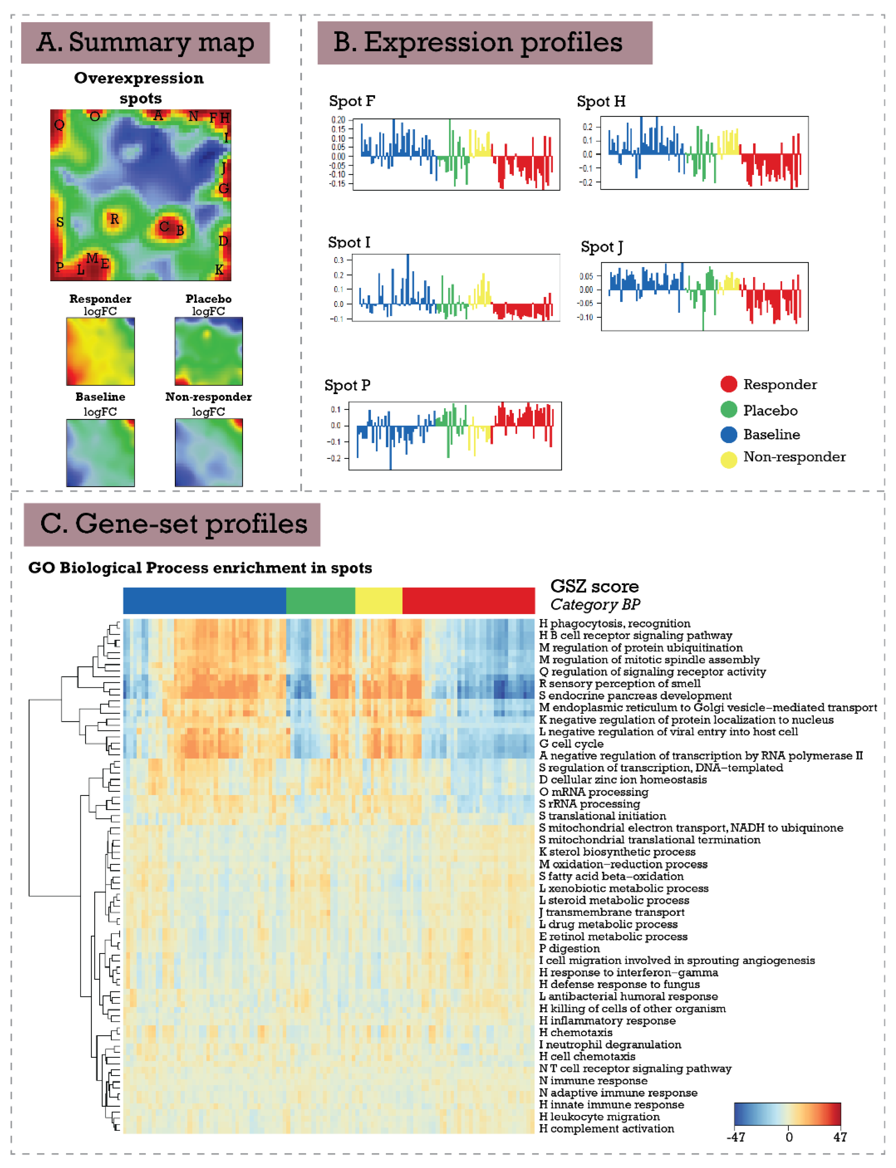
3.2. Inflammatory Bowel Disease (Ulcerative Colitis and Crohn’s Disease) Response to Infliximab—supSOM (Transferring Treatment Data to Disease Landscapes)

In this section, we used two publicly available datasets from the context of inflammatory colon diseases as an exemplary use case: GSE23597 (title: “Expression data from colonic biopsy samples of infliximab treated UC patients”) and GSE16879 (title: “Mucosal expression profiling in patients with inflammatory bowel disease before and after first infliximab treatment”). The GSE23597 dataset contains samples from patients with baseline ulcerative colitis (UC) disease, as well as patients treated with infliximab or placebo (54,613 genes × 113 samples). This dataset was used as a reference (primary data) for SOM training. The GSE16879 dataset contains samples from patients with UC and Crohn’s disease (CD) before and after treatment with infliximab (54,613 genes × 90 samples). This dataset was used as secondary data for the extension approaches in a second step. The samples in both datasets were additionally stratified to responders and nonresponders. SOM portrayal of the primary dataset demonstrated that infliximab responders and nonresponders showed distinct patterns of deregulation of functional spots on the SOM transcriptome landscapes (Figure 4). The SOM portraits of disease baseline (untreated), as well as nonresponder patients, were characterized by upregulated spots on the upper right corner of SOM maps (spot H and F), while responder patients were characterized by an overexpressed spot in the left bottom corner of the map (spot P). The functional analysis of deregulated modules suggests the upregulation of inflammatory response, particularly tumor necrosis factor (TNF) signaling pathway in baseline nontreated patients and nonresponders, in agreement with previous studies [21,22]. In contrast, patients who responded to infliximab showed marked downregulation of inflammation and upregulation of functional gene sets associated with tissue restoration and cell metabolism. Interestingly, the gene expression landscape in the placebo group was similar to that of patients receiving infliximab; however, the magnitude of spot expression was considerably lower. However, compared to the drug, the placebo group was still characterized by upregulation of immune/inflammatory gene signatures (Figure 4 and Figure S2), suggesting that infliximab possesses strong anti-inflammatory effects in responders, and, in parallel, induces injured tissue restoration by activating growth factor signaling and metabolic pathways.
Based on the SOM landscape obtained, we performed a supSOM and exSOM portrayal of gene expression in an independent dataset (GSE16879), which contained biopsy samples from patients with ulcerative colitis (UC) and Crohn’s disease (CD) before and after treatment with infliximab as well as normal colonic mucosa samples. In addition, patients were retrospectively stratified into infliximab responder and nonresponder groups [23]. supSOM (Figure 5) as well as exSOM (see Figure S3) portraits of UC patients after treatment showed perfect matching to the corresponding SOM portraits. Additionally, obtained results allowed for gaining additional insights into mechanisms of inflammatory bowel diseases and infliximab treatment efficacy. First, we observed considerable differences in the spot patterns observed in responder vs. nonresponder IBD patients before treatment (Figure 5). Both UC and CD nonresponder patients showed marked upregulation of immunity and inflammation-related signatures localized on the top right corner of the SOM portraits (corresponds to spots F, H, and I in primary SOM landscape, see Figure 4), particularly TNF signaling via TNFR2, pattern-recognition receptor signaling, nitric oxide synthesis, neutrophil activation, etc. (Supplementary Figure S4). Interestingly, baseline (before treatment) molecular portraits of UC and CD responder groups showed distinct patterns of up- and downregulated functional modules. The molecular portraits of CD responders were more similar to the healthy subjects (Pearson’s r = 0.74), compared to the UC responders (Pearson’s r = 0.09). Further analysis indicated that the UC and CD nonresponders were characterized by the increased baseline levels of TNF-a compared to the responders, however, with a similar tendency of expression decrease after treatment (Figure S5). This can indicate that not responding to the drug can be at least partially attributed to inadequate dosing of infliximab [24].

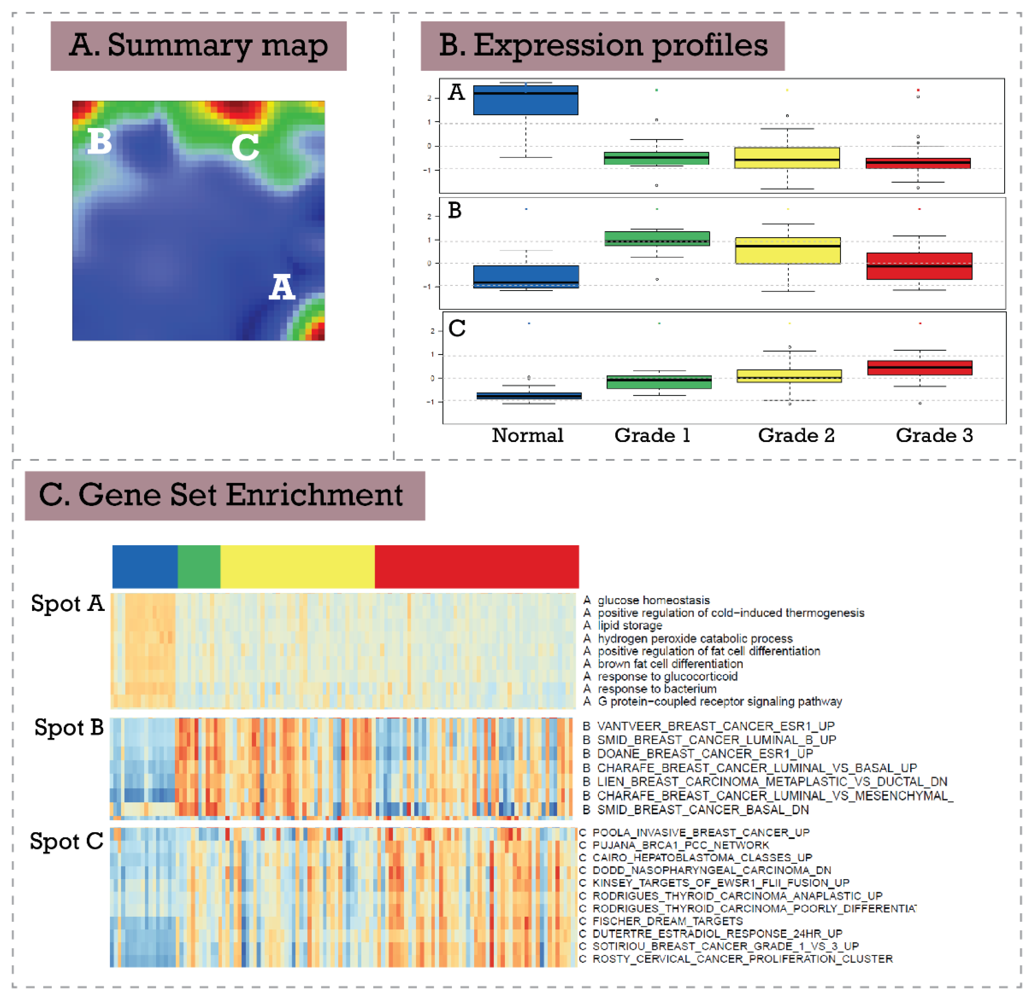
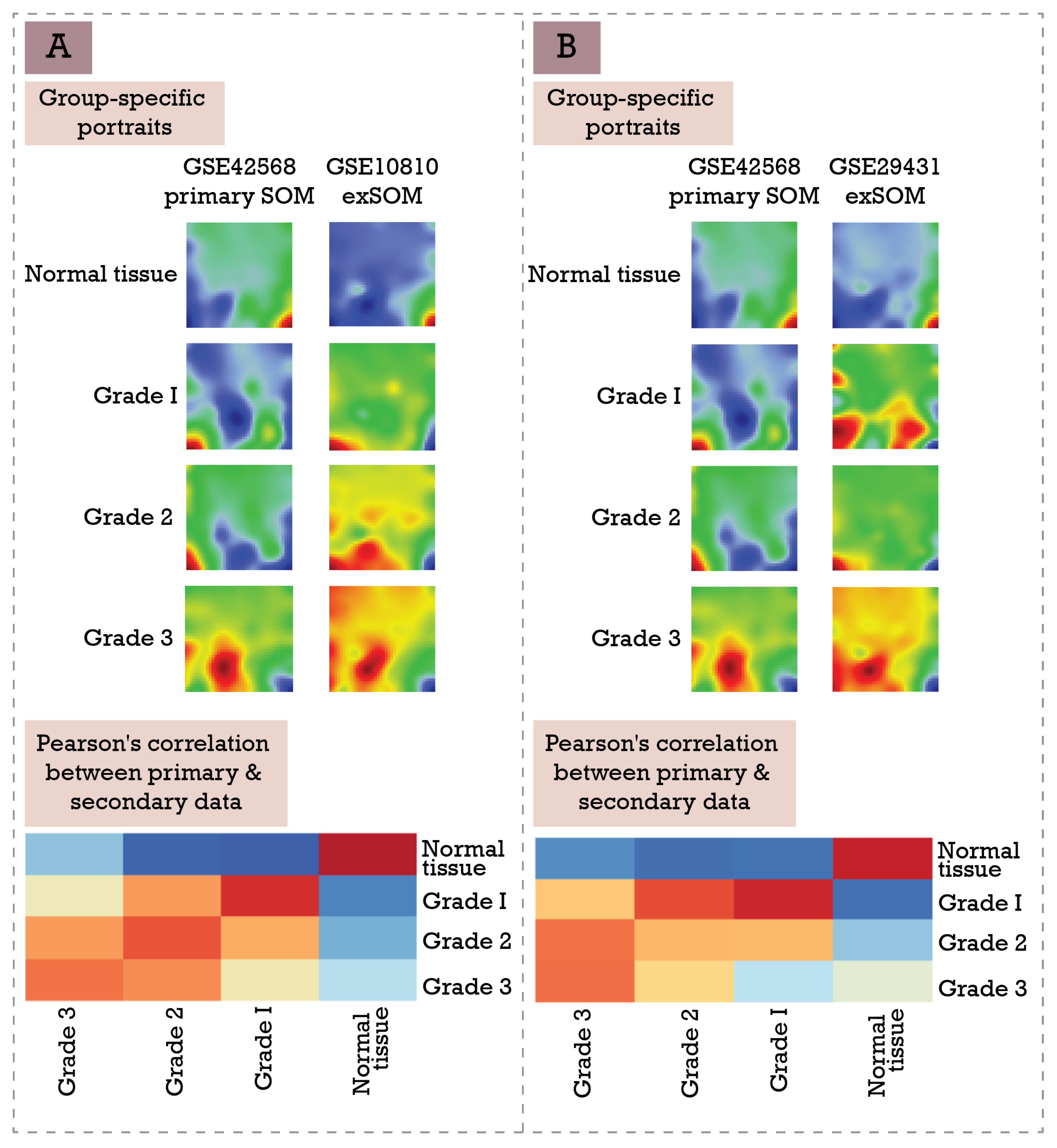
3.3. Extending Breast Cancer Transcriptome Landscapes—exSOM

As a second use case, we used the exSOM approach to perform disease grade-associated molecular portrayal of breast cancers. The GSE42568 dataset contains gene expression profiles measured in 121 healthy and breast cancer tissue samples. Samples were stratified by breast cancer histologic grading (17 normal, 11 Grade I, 40 Grade II, 53 Grade III) [25]. Using this dataset as primary, we performed 40 × 40 SOM training to cluster co-expressed genes and characterize transcriptome portraits of cancer grades. The results indicate that normal breast tissue expression signatures substantially differ from diseased ones (Figure 6A,B). Breast cancers were generally characterized by the loss of normal tissue gene expression (spot A), including response to hypoxia, lipid metabolism process, cell adhesion, and extracellular matrix organization. Moreover, we observed a grade-dependent increase in the number of differentially expressed genes (Figure S6). Furthermore, we also noticed switching cancer gene expression signatures from luminal to basal type (Figure 6C). Grade I cancers were characterized by upregulation of spot B associated with luminal type, response to estrogen, and immune response. Grade II cancers largely share gene expression signatures with Grade I and Grade III, representing a transition type without having a characteristic spot. The Grade III cancers were additionally characterized by upregulation of functional modules involved in cell proliferation, cell–cell adhesion, cell migration, and epithelial–mesenchymal transition (spots C) (Figure 6C).
Next, we used exSOM portrayal to map samples from two different secondary datasets (GSE29431 and GSE10810) to the primary SOM landscape. The GSE29431 dataset contained 51 samples (12 normal, 3 Grade I, 11 Grade II, and 25 Grade III); the GSE10810 dataset contained 47 samples (27 normal, 2 Grade I, 10 Grade II, and 10 Grade III). The exSOM, as well as supSOM portraits for both secondary datasets, showed a good correlation with primary SOM counterparts (Figure 7 and Figure S7). Moreover, exSOM portraits further emphasized the “indiscrete” pattern of Grade II breast cancers. In line with previous data, our results suggest that grades are not discrete but rather form a continuum with uncertain boundaries, which complicate classification and assignment [26,27,28] of this important prognostic marker.

4. Conclusions

In this paper, we described options for extending SOM-based high-dimensional transcriptomic data portraying with additional, independent samples. The two extension approaches presented enable overcoming the main limitation of SOM machine learning, namely, that adding samples or complete datasets changes the intrinsic primary structure of primary SOM. Both exSOM and supSOM demonstrated their utility in overcoming this drawback. Both methods have their advantages and disadvantages: while exSOM seems more accurate, supSOM is time-efficient.
From the methodical side, the novelty of the study is provided by the combination of previous SOM portrayal neural network machine learning with extrapolation of metagene values for novel samples using additive transfer learning approaches which transfer novel data into a multidimensional space obtained from previously collected data. The novel methods considerably widen the application range of SOM portrayal because they not only make computations more effective but, especially, because they enable usage of always analyzed data space for novel samples.
Analysis of inflammatory disease and cancer datasets demonstrated the validity of the projection methods with independent datasets mapped on existing SOM space. Moreover, we showed that the methods well handle the projection of samples with new characteristics that were not present in training datasets (see the “inflammatory bowel disease response to infliximab” section of the Results).
Thus, we demonstrated that SOM extension methods (exSOM and supSOM) can remarkably extend the usage scenarios of SOM “molecular data portrayal” approaches.

Supplementary Materials

The following are available online at https://0-www-mdpi-com.brum.beds.ac.uk/article/10.3390/biomedinformatics2010004/s1 Text S1: gives the codes for the generation of a simulated data set. Figure S1: Complete portrayal of simulated dataset with SOM, exSOM, and supSOM, Figure S2: Pairwise differential gene expression in primary SOM IBD dataset (GSE23597), Figure S3: Comparison of supSOM and exSOM portraits in secondary IBD dataset (GSE16879), Figure S4: Biological processes associated with upregulated spots F, H, and I on the primary SOM IBD dataset. Baseline disease and nonresponders were characterized with upregulated stops F, H, and I (see Figure 4) related to inflammatory response, cytokine-mediated signaling, neutrophil activation, reorganization, etc., Figure S5: Differential expression landscape in IDB responders vs. nonresponders in the secondary dataset (GSE16879). Orange color indicates upregulation, blue color indicates downregulation, white indicates the region of invariant gene expression, Figure S6: Grade-dependent change of differential expression genes in breast cancer, Figure S7: Comparison of exSOM and supSOM portraits in secondary breast cancer datasets. (A) GSE10810, (B) GSE29431.

Author Contributions

Conceptualization, A.A., H.L.-W., M.N., and H.B.; methodology, A.A. and H.L.-W.; formal analysis, S.D. and M.N.; data curation, A.A.; writing—original draft preparation, A.A., H.B., H.L.-W., M.N., and S.D.; visualization, M.N.; supervision, A.A.; funding acquisition, A.A. and M.N. All authors have read and agreed to the published version of the manuscript.

Funding

The work was supported by the Science Committee of RA in the frames of the projects 21AG-1F021 and 21SC-BRFFR-1F020 (to A.A.), and Armenian National Science and Education Fund in the frames of the project ANSEF compsci-2324 (to M.N.). The paper is supported by the State Target Program of the Government of the Republic of Armenia under grant agreement № 1-8/20TB project “Creating a Cloud Computing Environment for Solving Scientific and Applied Problems”.

Institutional Review Board Statement

Not applicable.

Informed Consent Statement

Not applicable.

Data Availability Statement

Raw data and scripts are available as supplementary datasets in the open-access repository Zenodo (https://zenodo.org/record/5736510, accessed on 1 December 2021) as well as supplementary materials of this article.

Conflicts of Interest

The authors declare no conflict of interest. The funders had no role in the design of the study; in the collection, analyses, or interpretation of data; in the writing of the manuscript, or in the decision to publish the results.

References

  1. Löffler-Wirth, H.; Kalcher, M.; Binder, H. oposSOM: R-package for high-dimensional portraying of genome-wide expression landscapes on bioconductor. Bioinformatics 2015, 31, 3225–3227. [Google Scholar] [CrossRef]
  2. Gomes, L.L.; Moreira, F.C.; Hamoy, I.G.; Santos, S.; Assumpção, P.; Santana, Á.L.; Santos, Â. Identification of miRNAs Expression Profile in Gastric Cancer Using Self-Organizing Maps (SOM). Bioinformation 2014, 10, 246–250. [Google Scholar] [CrossRef] [PubMed] [Green Version]
  3. Borkowska, E.M.; Kruk, A.; Jedrzejczyk, A.; Rozniecki, M.; Jablonowski, Z.; Traczyk, M.; Constantinou, M.; Banaszkiewicz, M.; Pietrusinski, M.; Sosnowski, M.; et al. Molecular subtyping of bladder cancer using Kohonen self-organizing maps. Cancer Med. 2014, 3, 1225–1234. [Google Scholar] [CrossRef] [PubMed]
  4. Schmidt, M.; Hopp, L.; Arakelyan, A.; Kirsten, H.; Engel, C.; Wirkner, K.; Krohn, K.; Burkhardt, R.; Thiery, J.; Loeffler, M.; et al. The Human Blood Transcriptome in a Large Population Cohort and Its Relation to Aging and Health. Front. Big Data 2020, 3, 36. [Google Scholar] [CrossRef] [PubMed]
  5. Jansen, C.; Ramirez, R.N.; El-Ali, N.C.; Gomez-Cabrero, D.; Tegner, J.; Merkenschlager, M.; Conesa, A.; Mortazavi, A. Building gene regulatory networks from scATAC-seq and scRNA-seq using Linked Self Organizing Maps. PLoS Comput. Biol. 2019, 15, e1006555. [Google Scholar] [CrossRef] [PubMed] [Green Version]
  6. Binder, H.; Wirth, H. Analysis of large-scale omic data using self organizing maps. In Encyclopedia of Information Science and Technology, 3rd ed.; IGI Global: Pennsylvania, PA, USA, 2014; pp. 1642–1653. [Google Scholar]
  7. Delgado, S.; Morán, F.; Mora, A.; Merelo, J.J.; Briones, C. A novel representation of genomic sequences for taxonomic clustering and visualization by means of self-organizing maps. Bioinformatics 2014, 31, 736–744. [Google Scholar] [CrossRef] [Green Version]
  8. Steiner, L.; Hopp, L.; Wirth, H.; Galle, J.; Binder, H.; Prohaska, S.J.; Rohlf, T. A Global Genome Segmentation Method for Exploration of Epigenetic Patterns. PLoS ONE 2012, 7, e46811. [Google Scholar] [CrossRef] [Green Version]
  9. Peng, T.; Nie, Q. SOMSC: Self-Organization-Map for High-Dimensional Single-Cell Data of Cellular States and Their Transitions. bioRxiv 2017, 124693. [Google Scholar] [CrossRef] [Green Version]
  10. Rallo, R.; France, B.; Liu, R.; Nair, S.; George, S.; Damoiseaux, R.; Giralt, F.; Nel, A.; Bradley, K.; Cohen, Y. Self-organizing map analysis of toxicity-related cell signaling pathways for metal and metal oxide nanoparticles. Environ. Sci. Technol. 2011, 45, 1695–1702. [Google Scholar] [CrossRef] [Green Version]
  11. Zhang, J.; Fang, H. Using Self-Organizing Maps to Visualize, Filter and Cluster Multidimensional Bio-Omics Data. In Applications of Self-Organizing Maps; IntechOpen Limited: London, UK, 2012; pp. 181–204. [Google Scholar]
  12. Kunz, M.; Löffler-Wirth, H.; Dannemann, M.; Willscher, E.; Doose, G.; Kelso, J.; Kottek, T.; Nickel, B.; Hopp, L.; Landsberg, J.; et al. RNA-seq analysis identifies different transcriptomic types and developmental trajectories of primary melanomas. Oncogene 2018, 37, 6136–6151. [Google Scholar] [CrossRef]
  13. Binder, H.; Willscher, E.; Loeffler-Wirth, H.; Hopp, L.; Jones, D.T.W.; Pfister, S.M.; Kreuz, M.; Gramatzki, D.; Fortenbacher, E.; Hentschel, B.; et al. DNA methylation, transcriptome and genetic copy number signatures of diffuse cerebral WHO grade II/III gliomas resolve cancer heterogeneity and development. Acta Neuropathol. Commun. 2019, 7, 59. [Google Scholar] [CrossRef] [Green Version]
  14. Wirth, H.; Von Bergen, M.; Binder, H. Mining SOM expression portraits: Feature selection and integrating concepts of molecular function. BioData Min. 2012, 5, 18. [Google Scholar] [CrossRef] [PubMed] [Green Version]
  15. Wirth, H.; Löffler, M.; von Bergen, M.; Binder, H. Expression cartography of human tissues using self organizing maps. BMC Bioinformatics 2011, 12, 306. [Google Scholar] [CrossRef] [Green Version]
  16. Koutník, J.; Šnorek, M. Temporal Hebbian self-organizing map for sequences. In Proceedings of the Lecture Notes in Computer Science (Including Subseries Lecture Notes in Artificial Intelligence and Lecture Notes in Bioinformatics), Torun, Poland, 25–29 August 2008. [Google Scholar]
  17. Dembélé, D. A Flexible Microarray Data Simulation Model. Microarrays 2013, 2, 115–130. [Google Scholar] [CrossRef] [PubMed] [Green Version]
  18. Edgar, R.; Lash, A. The Gene Expression Omnibus (GEO): A Gene Expression and Hybridization Repository. Nucleic Acids Res. 2002, 6, 1–17. [Google Scholar] [CrossRef] [Green Version]
  19. Nikoghosyan, M.; Loeffler-Wirth, H.; Davitavyan, S.; Binder, H.; Arakelyan, A. Projection of High-Dimensional Genome-Wide Expression on SOM Transcriptome Landscapes: Supplementary Datasets. Zenodo 2021. [Google Scholar] [CrossRef]
  20. Braga-Neto, U.; Dougherty, E. Bolstered error estimation. Pattern Recognit. 2004, 37, 1267–1281. [Google Scholar] [CrossRef]
  21. Christophi, G.P.; Rong, R.; Holtzapple, P.G.; Massa, P.T.; Landas, S.K. Immune Markers and Differential Signaling Networks in Ulcerative Colitis and Crohn’s Disease. Inflamm. Bowel Dis. 2012, 18, 2342–2356. [Google Scholar] [CrossRef] [PubMed] [Green Version]
  22. Wilhelm, S.M.; McKenney, K.A.; Rivait, K.N.; Kale-Pradhan, P.B. A review of infliximab use in ulcerative colitis. Clin. Ther. 2008, 30, 223–230. [Google Scholar] [CrossRef]
  23. Arijs, I.; De Hertogh, G.; Lemaire, K.; Quintens, R.; Van Lommel, L.; Van Steen, K.; Leemans, P.; Cleynen, I.; Van Assche, G.; Vermeire, S.; et al. Mucosal gene expression of antimicrobial peptides in inflammatory bowel disease before and after first infliximab treatment. PLoS ONE 2009, 4, e7984. [Google Scholar] [CrossRef]
  24. Wong, U.; Cross, R.K. Primary and secondary nonresponse to infliximab: Mechanisms and countermeasures. Expert Opin. Drug Metab. Toxicol. 2017, 13, 1039–1046. [Google Scholar] [CrossRef] [PubMed]
  25. Clarke, C.; Madden, S.F.; Doolan, P.; Aherne, S.T.; Joyce, H.; O’Driscoll, L.; Gallagher, W.M.; Hennessy, B.T.; Moriarty, M.; Crown, J.; et al. Correlating transcriptional networks to breast cancer survival: A large-scale coexpression analysis. Carcinogenesis 2013, 34, 2300–2308. [Google Scholar] [CrossRef] [PubMed]
  26. Sotiriou, C.; Wirapati, P.; Loi, S.; Harris, A.; Fox, S.; Smeds, J.; Nordgren, H.; Farmer, P.; Praz, V.; Haibe-Kains, B.; et al. Gene expression profiling in breast cancer: Understanding the molecular basis of histologic grade to improve prognosis. J. Natl. Cancer Inst. 2006, 98, 262–272. [Google Scholar] [CrossRef] [PubMed]
  27. Ignatiadis, M.; Sotiriou, C. Understanding the molecular basis of histologic grade. Pathobiology 2008, 75, 104–111. [Google Scholar] [CrossRef]
  28. Lu, X.; Lu, X.; Wang, Z.C.; Iglehart, J.D.; Zhang, X.; Richardson, A.L. Predicting features of breast cancer with gene expression patterns. Breast Cancer Res. Treat. 2008, 108, 191–201. [Google Scholar] [CrossRef] [PubMed]
Figure 1. General workflow of exSOM and supSOM algorithms. (A) For both algorithms, the first step is SOM training with the primary dataset. (B) In exSOM, “secondary” data is added to the existing SOM space by passive training. (C) In supSOM, the SVMR model is trained to map the primary dataset to its SOM “portraits”. (D) During supSOM testing, the “secondary” dataset is supplied to the model for projection into the SOM space. Single arrows indicate the order in the pipeline, while double arrows the dimensions of samples/features in the matrix.
Biomedinformatics 02 00004 g001
Figure 2. Performance of exSOM transfer learning using “self-portraying”. (A) exSOM adapts secondary data to an existing SOM via passive training of the meta-genes. First, SOM arranges primary data (black lines in the top-right pane) on the grid, while secondary data (grey line in the top-right pane) do not contribute to gene clustering. During the extension phase, the secondary data is mapped to the existing SOM grid (black line on the bottom right pane). (B) The meta-gene adaptation of secondary data results in identical images compared to the corresponding sample in the primary data. (C) The correlation between paired samples from primary and secondary datasets showed perfect matching (Pearson’s correlation coefficients equal 1 (red diagonal in the heatmap) and RMSD equal to 0, not shown).
Biomedinformatics 02 00004 g002
Figure 3. Performance of supSOM transfer learning using “self-portraying”. (A) supSOM utilizes support vector machine regression to train the primary dataset with the corresponding meta-genes. Single arrows indicate the order in the pipeline, while double arrows the dimensions of sam-ples/features in the matrix. (B) The trained models are then used for the prediction of meta-gene values of the secondary data. (C) The performance of supSOM portrayal depends on the neighborhood radius. The optimal radius value was selected equal to 4 (red arrow) based on RMSD and Pearson’s correlation. (D) supSOM portrayal shows slight differences compared to original SOM. The white areas on the maps represent meta-genes where the prediction failed. (E) The correlation heatmap between paired samples from primary and secondary datasets showed good matching (Pearson’s correlation coefficients close to 1 (red diagonal in the heatmap).
Biomedinformatics 02 00004 g003
Figure 4. Transcriptome landscape (primary SOM space) of response to infliximab in ulcerative colitis. (A) The overview map is segmented into 19 modules, from which 5 modules (F, H, I, J, and P) were deregulated in a group-specific manner. Group-specific mean transcriptome portraits of studied groups (see [15]). (B) Module (spot)-specific expression profiles in groups. The results show that modules F, H, and I were upregulated in the baseline disease and nonresponder group, while the expression of modules P and J were upregulated in responders. (C) The heatmap of module-specific gene-set enrichment scores. The results indicate that drug responders and nonresponders show differential deregulation of gene modules that are associated with inflammation, TNF-alpha signaling (spots F, H, and I), tissue restoration, and cell metabolism (spot P).
Biomedinformatics 02 00004 g004
Figure 5. Projection of GSE16879 (mucosal expression profiling in patients with inflammatory bowel disease before and after first infliximab treatment) dataset onto primary SOM space. supSOM portraits of UC patients after treatment showed perfect matching to the corresponding portraits of the original SOM. supSOM portraits highlight the differences in deregulated spots between responder and nonresponder IBD patients before treatment. Both UC and CD nonresponders are characterized by an overexpressed spot on the top-right corner of their corresponding group portraits, which remains unchanged after treatment. In contrast, US and CD responders showed a different distribution of upregulated spots before treatment, while their corresponding portraits after treatment resemble transcriptome portraits of healthy mucosa.
Biomedinformatics 02 00004 g005
Figure 6. Primary SOM transcriptome landscape of disease grade-stratified breast cancers. (A) Overview map of deregulated functional gene modules in primary SOM. (B) Group-specific module expression. (C) Heatmap of enrichment analysis scores of functional modules.
Biomedinformatics 02 00004 g006
Figure 7. Comparison of exSOM portrayal of breast cancer transcriptome landscapes. (A) Portrayal of GSE42568 (primary) and GSE10810 (secondary/extension). (B) Portrayal of GSE42568 (primary) and GSE29431 (extension).
Biomedinformatics 02 00004 g007
Table 1. SOM training times for gene expression matrices of different sizes.
n = 10,000 Genes n = 30,000 Genes
Sample Size
(Control/Case)
Training TimeSample Size
(Control/Case)
Training Time
50/503 min50/508 min
100/1008 min100/10016 min
200/20014 min200/20037 min
500/50043 min500/500116 min
1000/100085 min1000/1000228 min
Table 2. Comparison of computational time of exSOM and supSOM.
Data—200 Samples in Each Class with 30,000 GenesTime
exSOM23 min
SOM training (50/50 samples)8 min
extSOM (150/150 samples)15 min
supSOM14 min
SOM training 50/50 samples8 min
SVMR model training (50/50 samples)4 min
SVMR portrait prediction (150/150 samples)2 min
Publisher’s Note: MDPI stays neutral with regard to jurisdictional claims in published maps and institutional affiliations.

