
Short-Term Traffic Forecasting: An LSTM Network for Spatial-Temporal Speed Prediction


1
Department of Civil and Construction Engineering, Swinburne University of Technology, Hawthorn, VIC 3122, Australia
2
Department of Computer Science and Software Engineering, Swinburne University of Technology, Hawthorn, VIC 3122, Australia
*
Author to whom correspondence should be addressed.
Future Transp. 2021, 1(1), 21-37; https://0-doi-org.brum.beds.ac.uk/10.3390/futuretransp1010003
Submission received: 5 January 2021
/
Revised: 19 February 2021
/
Accepted: 5 March 2021
/
Published: 30 March 2021
Abstract
:Traffic forecasting remains an active area of research in the transport and data science fields. Decision-makers rely on traffic forecasting models for both policy-making and operational management of transport facilities. The wealth of spatial and temporal real-time data increasingly available from traffic sensors on roads provides a valuable source of information for policymakers. This paper adopts the Long Short-Term Memory (LSTM) recurrent neural network to predict speed by considering both the spatial and temporal characteristics of real-time sensor data. A total of 288,653 real-life traffic measurements were collected from detector stations on the Eastern Freeway in Melbourne/Australia. A comparative performance analysis among different models such as the Recurrent Neural Network (RNN) that has an internal memory that is able to remember its inputs and Deep Learning Backpropagation (DLBP) neural network approaches are also reported. The LSTM results showed average accuracies in the outbound direction ranging between 88 and 99 percent over prediction horizons between 5 and 60 min, and average accuracies between 96 and 98 percent in the inbound direction. The models also showed resilience in accuracies as the prediction horizons increased spatially for distances up to 15 km, providing a remarkable performance compared to other models tested. These results demonstrate the superior performance of LSTM models in capturing the spatial and temporal traffic dynamics, providing decision-makers with robust models to plan and manage transport facilities more effectively.
1. Introduction
The new technologies and advances in data analytics are providing innovative ways to sense and manage transport networks. The fast pace of breakthroughs in these technologies, including artificial intelligence and machine learning, is relentless and continues to unfold on many fronts. By determining when and how to take advantage of these technologies, policymakers and decision-makers have unique opportunities to enhance people’s access to services and facilities, improve travel time reliability for road users, and enhance the economic and infrastructure productivity of vital infrastructure assets [1]. Short-term traffic forecasting has been an active area of research for more than three decades and has been discussed widely in the literature using a variety of theoretical models based on either simulated or field data [2]. Field data can be most useful for model development [1,3] but can be difficult to collect such that the spatial and temporal characteristics are captured. In the absence of reliable field data, many studies reported in the literature have instead used simulated data generated from well-calibrated and validated traffic simulation models [4]. Although a large number of studies have used advanced computational models to develop accurate forecasting methods that deal with the complexity of massive amounts of data, the literature on comparative evaluations of different models based on the same set of data is scarce. The ability to undertake such comparative evaluations based on the same set of field data to be used for short-term traffic forecasting will help identify models, which in turn can improve road user experience and enhance operational capabilities.
This paper demonstrates the feasibility of using advanced AI techniques for short-term traffic forecasting, taking into consideration the spatial and temporal characteristic of the data using the Long Short-Term Memory (LSTM) prediction network. This model is developed using historical data extracted from 8 upstream and downstream detector stations in Eastern Freeway, Melbourne, Australia.
Contribution
The objective of this paper is to develop and evaluate robust models that can be used by policy and decision-makers to plan and manage transport facilities in an effective manner. While the topic of traffic forecasting has received considerable attention in the past, the literature that examines the spatial and temporal interactions of traffic phenomena remains scarce. Hence, this paper considers the locations between each detector station and evaluates the effectiveness of the proposed model considering the influence of locations as well as the temporal evolution of traffic. Another key contribution, which has not been investigated before, is the feasibility of replicating models that have been developed for a particular location to other locations. This type of analysis is important when the input data of one location is missing. From a practical perspective, the ability to forecast and predict traffic conditions helps decision-makers plan ahead rather than rely on existing reactive systems that do not have any predictive capability. Another contribution of this paper is the development and evaluation of spatial-temporal traffic forecasting models using large field data sets (288,653 observations) that have been validated from multiple locations on the road network in Melbourne.
This paper is organised as follows: Section 2 provides a scan of the literature on the topic. Section 3 discusses the model formulation and modelling architectures used in the study. Section 4 describes a case study that includes data collection and pre-processing, and model evaluation, including results and findings. Finally, Section 5 presents conclusions and future research directions.
2. Literature Review
The reform of urban mobility still presents major challenges to policymakers around the world. Despite years of investment in road infrastructure, the traditional approach of focusing on building out of congestion through additional road capacity did not meet with much success. In recent times, more focus has been given to managing the demand for travel. Among the many demand management solutions, pro-active or predictive traffic forecasting has been identified as an essential component of improving traffic conditions [5]. In short-term traffic forecasting, estimating traffic conditions usually focuses on speed and flow predictions. Speed prediction, in particular, is directly related to proactive traffic control system development [6,7]. However, estimating vehicle speed is problematic because it is affected by driver behaviour, road environment and the spatial and temporal complexities of traffic conditions. Solving this complex and uncertain speed prediction problem has been the focus of many studies in the literature [8,9]. Methodologies used for speed prediction can be classified into two categories or approaches: parametric and non-parametric [10]. These are discussed next.
2.1. Parametric Approaches
The parametric approaches, also known as model-based methods, are based on certain theoretical assumptions of the predetermined model structure. The model parameters can be computed using empirical data [11,12]. Most commonly used parametric time-series analysis approaches include linear models such as the Autoregressive Integrated Moving Average model (ARIMA) [13], seasonal ARIMA, that is, the SARIMA model [14], the exponential smoothing model [15,16] and ARIMA with a Kalman filter (KF) [17,18]. In an early reference [19], the authors found the ARIMA model was capable of representing freeway time-series data accurately. Numerous extended models of ARIMA have emerged due to its superiority in forecasting traffic dynamics [20,21]. These parametric approaches require high-quality data where the sequence needed to be stable and accurate. As most real-life traffic data are unstable and stochastic, this has limited their use and applicability in complex traffic prediction applications [22].
2.2. Non-Parametric Approaches
Non-parametric approaches distinctly predict traffic conditions as these models do not consist of fixed model structures and parameters [23]. Specifically, non-parametric methods contain relaxed assumptions for inputs and are hence are more capable of processing missing data, noisy data and outliers [24]. With the recent advancements in machine learning, many models have shown great potential in solving non-linear problems even when using complex and multi-source field data. Such models include Support Vector Regression (SVR) [25,26,27] and Artificial Neural Networks (ANNs) [28,29].
For example, Ref. [30] compared four parametric approaches (Constant Speed (CS), Constant Acceleration (CA), SUMO simulator model SUMO, and Intelligent Driver Model (IDM)) and two non-parametric approaches (Gaussian Mixture Regression (GMR) and the Artificial Neural Network (ANN) technique) to forecast speeds on highways. The results showed non-parametric models consistently outperformed other models for both short and long term predictions. Compared to parametric approaches, non-parametric approaches can result in higher accuracies [31], particularly, neural networks that showed the best prediction results [32]. In another comparative study [33], Back-Propagation Neural Networks (BPNNs) and traditional approaches were compared, and the results showed the BPNN to be superior and more responsive to dynamic conditions. Therefore, for complex, non-linear problems like traffic prediction, ANN models are more accurate with stronger capabilities for learning the association of multi-variant inputs and output patterns [34]. In another study [30] that compared different neural network architectures, the authors’ General Regression Neural Network (GRNN) was shown to be simple, stable, and descriptive of dynamic system characteristics [35].
Recently, novel architectures of neural networks such as the Long Short-Term Memory (LSTM) and Recurrent Neural Networks (RNNs) have attracted research interest as effective tools for traffic prediction [11,36,37]. For example, an RNN combined with LSTM traffic prediction [11] was found to provide higher performance compared to classical methods. Focusing on speed of individual vehicles, Ref. [36] used an RNN with LSTM and developed a car-following model to predict acceleration on roads. Other researchers have also developed LSTM-based RNN approaches for speed prediction models under various urban driving conditions with credible and accurate results [38].
Unlike previously mentioned studies which lacked the spatial consideration of the traffic state correlations, and with the availability of enriched traffic data, this paper extends more recent work that exploits the spatial and temporal traffic state features to develop robust traffic forecasting models. Some of the previous notable research where spatial-temporal characteristics were explored includes different approaches. For example, Ref. [39] developed a model based on the LSTM-NN, using graph convolution to mine spatial-temporal features. Also, Ref. [40] converted network traffic to images, where they also used predictive models to estimate future scenarios. Furthermore, Ref. [41] incorporated spatial and temporal patterns in short-term forecasting in traffic volume based on Modular Neural Networks (MNNs). However, it is difficult to establish from these studies, which were developed using different data sets, which models perform better and under which set of conditions. This limitation is addressed in this paper by considering six NN models that were trained, tested and validated based on a unique set of field observations with varying spatial and temporal state features by considering the locations between sensor stations and evaluating the effectiveness of the proposed models for both time and space analysis.
3. Model Development
The road facility is divided spatially into sections bounded by detector stations. The data for each detector location is then categorized into different time horizons {5, 10, 15, 30, 45 and 60} minutes. The goal is to predict the spatial and temporal information of the next time stamp (t + n) where n ranges from 5 to 60 min into the future with consideration to the spatial location for each detector, as shown in Figure 1.
Long Short-Term Memory (LSTM)
The RNN architecture described before provides good accuracy but does not perform well for long-term memory, as the RNNs are unable to use information from a distant past. To address this problem, Long Short-Term Memory (LSTM) models are considered extensions of the RNN to overcome these issues. Also, LSTM models can learn patterns with long dependencies when compared with traditional RNNs, that are not able to function for long term patterns. Therefore, the LSTM has generally been found to outperform RNNs in time series data forecasting [38].
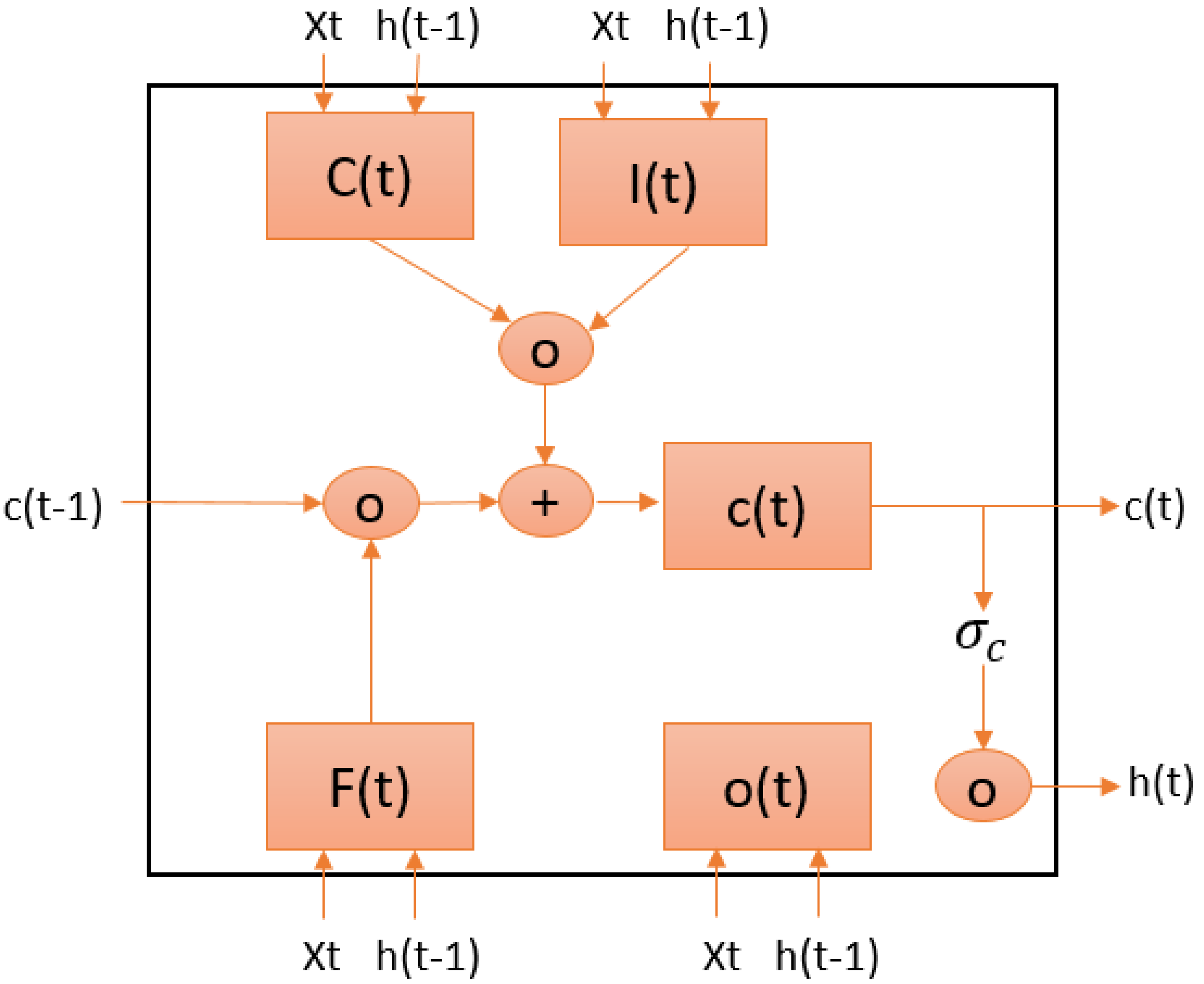
LSTM models have a different structure from RNNs, as shown in the architecture presented in Figure 2. The following formulae are used to calculate the predicted values:
where σg is the gate activation function, are input weight matrices, are recurrent weight matrices, is the input, is the output at the previous time (t − 1), and are bias vectors. The forget gate determines how much of the prior memory values should be removed from the cell state. Similarly, the input gate specifies new input to the cell state. Then, the cell state ct and the output ht of the LSTM at time t is calculated as follows:
where ⊙ denotes the Hadamard product (element-wise multiplication of vectors).
ct = ft⊙ct − 1 + it⊙gt
ht = ot⊙σc(ct)
For this work, the LSTM was implemented in Matlab [43]. First, the data for temporal prediction were arranged for each detector as two-column values; the first column corresponded to speed at time (t), and the second column corresponded to the expected output (t + n) where n ranges from 5 to 60 min into the future. For spatial prediction, the data were also arranged as two-column values. However, the first column represented the speed at time (t) for the detector (r) and the second column represented the expected output of the speed at the time (t) for the following detector (r + 1).
Then, the data were partitioned into the training and test data. The model was trained on the first 60% of the sequence and tested on the last 40%. To prevent the model from overfitting, the training/testing data were standardised to have zero mean and unit variance. After that, the LSTM network is created using four layers: Sequence Input Layer (number of features = 1), LSTM Layer (number of hidden units = 300), Fully Connected Layer (number of responses = 1) and a Regression Layer. The model parameter settings, as reported in Table 1. The tanh and sigmoid functions are used for state and gate activation functions, respectively. The LSTM experiments are implemented with Matlab R2019b with the Deep Learning Toolbox functions of trainNetwork, training options, and predictAndUpdateState.
4. Case Study Using Field Data from the Eastern Freeway (Melbourne/Australia)
This section presents a case study that demonstrates the proposed model’s applicability and its robustness and effectiveness using field data collected from the Eastern Freeway in Melbourne/Australia. This section first describes the data collection and characteristics of the field data and then presents a comparative evaluation of the model’s performance, including a detailed analysis of prediction results.
4.1. Data Collection
The real-life data used for the model development was collected from inductive loops embedded along the Eastern Freeway in Melbourne/Australia (Figure 3). This road facility is an 18-km freeway which is bounded by East Link at Nunawading (eastbound) and Alexandra Parade (westbound). The data used in this study included speed observations collected for 31 days from 1 July 2016 to 31 July 2016 for both eastbound (EB) and westbound (WB) directions. The data was aggregated every 1-min interval across all lanes at each site for each 24-h duration. Four different locations of detectors were chosen for each direction (8 locations in total), distributed across the mainline carriageway covering the entire freeway. It should be noted here that this is the most recent data available to the research team. This is not because of a lack of field data but because of the time and effort it takes to clean new field data and label it for such AI applications. The data described in this paper has been extensively cleaned with considerable time spent on ensuring that only quality data for the incident and non-incident conditions are used in model development and evaluation. Locations of detectors are shown in Figure 3 and Table 2.
Data for Model Development
The speed data used in the model development was gathered from four detection stations (14010 EB, 14028 EB, 14045 EB and 14061 EB). These locations were separated by distances of 5.0, 5.4 and 4.0 km intervals consecutively as shown in Figure 4. Also, four detection stations in the westbound direction (14061 WB, 14051 WB, 14031 WB and 14003 WB) were also approximately 5.4, 6.1 and 7.1 km apart as shown in Figure 4.
The data was aggregated at 1-min intervals across all lanes at each site. Considerable effort was given to pre-processing the data, including the removal of missing or corrupted data. For example, if the data was continuously missing for more than 10 min, the traffic values were removed. However, if the missing data was only for a short duration, for example, between (12 July 2016 17:48 and 12 July 2016 17:50), then the value at 12 July 2016 17:49 was estimated as:
Speed (t) = (Speed (t − 1) + Speed (t + 1))/2
The reason for choosing these four detectors for each direction is that they had the most reliable data with few missing observations for the 31-day duration. They were also chosen to capture variable spatial locations and traffic characteristics along the freeway for this research; the total number of valid observation for the eight detectors was 288,653 observations. For each detector, the data was divided into three data sets: Training (60%) and testing and validation (40%). The number of speed data tested for each detector (after pre-processing) is presented in Table 3. The training set was used to “calibrate” the neural network model in order to learn the traffic patterns. Using this data, the model learned from the relationships between the different variables in the input values. The testing data (which was not used for model training and calibration) was used to validate the results and ensure that the neural network was not memorising the patterns and the outputs from the training data set.
4.2. Model Evaluation
To evaluate Long Short-Term Memory (LSTM) prediction robustness, five machine learning systems were evaluated using the same data set. These included: Recurrent Neural Networks (RNNs), General Regression Neural Networks (GRNNs), Modular Neural Networks (MNNs), Deep Learning Backpropagation (DLBP) neural networks and Radial Basis Function Networks (RBFNs). These models have been widely used for future traffic forecasts, as shown in the example papers provided in the literature review section above. The models reported in this paper were developed using NeuralWorks Professional, which is an Artificial Neural Network commercial package and development system [45].
The Backpropagation Neural Network is the most popular learning algorithm used to capture non-linear relationships and self-learning. The typical back-propagation network always has an input layer, an output layer and more than one hidden layer, which is referred to as “Deep Learning”. Each layer is fully connected to the succeeding layer. The implementation of the algorithm simply includes an input training pattern (feedforward), backpropagated error and weight adjustment. The parameters used for this experiment included 3 hidden layers with 4, 6, and 2 neurons. The transfer function is Tanh with a learning coefficient output (α = 0.15). The learning rule is Ext DBD with 100,000 iterations and a momentum of 0.4.
The training for the Radial Basis Function Network (RBFN) network uses a radial basis function instead of a linear function with more neurons needed in the hidden layer compared to the multi-layer BP neural network. In general, an RBFN is any network which has an internal representation of hidden neurons (pattern units) which are radially symmetric. In order for a pattern unit to be radially symmetric, it should include the following criteria: a center, a distance measure and a transfer function. A center is vector in the input space and which is typically stored in the weight vector from the input layer to the pattern unit. The distance measure determines how far an input vector is from the center, such as the Euclidean distance measure. In terms of the transfer function, it determines the output by mapping the output of the distance function, such as the Gaussian function. The following parameters are used in this experiment: proto (50), summation function (Euclidean), momentum (0.4), learn rule (Ext DBD) and transfer (Tanh).
Modular Neural Network (MNN) models include modules and a gating network. The modules are referred to as “local experts” which approach the problem from various angles. The gating network is an integrated unit that allocates different features of the input space to the different local expert networks. The parameters chosen in this experiment were: hidden layers (1) with (14) neurons, and the activation function (tanh). Momentum (0.4), learn rule (ext DBD), learning rate hidden layer (0.3) and output layer (0.15), epoch (16), input vector [−1, +1] and output vector [−0.8, +0.8].
The General Regression Neural Network (GRNN) is a general purpose network paradigm based on linear regression theories but extends the regression to avoid assuming a specific functional form (such as linear) for the relationship between the inputs and outputs. The following parameters were used in this experiment: pattern neurons (50), summation function (Euclidean), radius of influence (R 0.250), σ scale (1), σ exponent (0.5) and Tau time constant (1000).
RNNs are feedforward neural networks that perform well with time series forecasting data. The type of RNN used is a Werbos RNN, in which the weights are updated by using the standard back-propagation algorithm. The parameters used for this experiment were: hidden layers (1) with (5) neurons, activation function (tanh), learn rule (ext DBD) and epoch (770). Finally, the reader is referred to a number of other references [46,47] that provide further details about the use of the Neuralware platform for automated incident detection and to a number of other studies that are relevant to the use of simulation tools [48,49,50,51,52,53,54] and how they can be used for evaluation of different transport management strategies to enhance efficiency and reduce emissions.
Also, it is essential to establish metrics that allow the comparison of the different methods. In this paper, the Mean Absolute Percentage Error (MAPE) is used to calculate the accuracy of the model prediction for different time horizons in the future. MAPE calculates the average absolute difference between the predicted output from the model (Y1) and the expected true output (Y) [55].
Accuracy (%) = (1 − MAPE) × 100
4.2.1. Westbound Direction—Temporal Prediction Accuracies
The experimental results for temporal variations in the westbound direction are provided in Table 4 and Figure 7. The cells in the table that are highlighted in green show the highest accuracies obtained, while the cells highlighted in orange show the lowest. The results show that the LSTM generally has superior performance when compared to the RNN, GRNN, MNN, RBF and the DLBP neural network.
For detector 14003, the results show that LSTM provides a forecasting accuracy of 94.24% for a 5-min prediction horizon and 94.97% for a 60-min prediction horizon. For the LSTM, the accuracy does not deteriorate substantially as the prediction horizon increases, with the accuracy remaining high at 94.97% for the 60-min horizon. This shows the ability of the system to capture the complexity of longer speed prediction horizons. On the other hand, the MNN provided the least accurate predictions out of the six models tested. For detector 14031, the same trend can be noticed with accuracies not deteriorating substantially for the LSTM with longer prediction horizons. For the 10-min horizon, the accuracy is 97.55%, while it remained steady at 98.96% for the 60-min horizon. Also, it can be noted that the LSTM provides better accuracy for 10 min and 60 min prediction horizons while the GRNN, MNN and RBF outperformed the LSTM for the other prediction horizons. This may be attributed to the data patterns for detector 14031, which showed more congestion at certain times during the months of July compared with other detectors. For longer prediction horizons (45 and 60 min), the DLBP neural network had the lowest performance of 95.22% and 94.14%, respectively.
For detector 14051, the LSTM outperforms all other 6 models with an accuracy ranging from 95.61% to 99.94%. The DLBP neural network and the MNN provided the least accuracies for shorter prediction horizons up to 30 min, while the RBF had the lowest accuracy of 89.72% compared to 99.94% of the LSTM for 45 min into the future. The RNN provided the least accurate predictions for 60-min horizons with 83.16% accuracy compared to 99.43% for the LSTM.
For detector 14063, the LSTM provided a good level of accuracy for all time horizons ranging from 97.68% to 98.77%. The DLBP neural network achieved the lowest accuracy for 15, 30 and 45 min predictions compared to the six models, whereas the RBF had the lowest accuracy for 60-min horizons (91.77%) compared with the LSTM with the highest accuracy of 98.77%.
4.2.2. Westbound Direction—Spatial Prediction Accuracies
For the spatial analysis, the main observation is that the accuracy of prediction is not affected as the distance between detector locations increases (Table 5 and Figure 8). The LSTM provides the highest accuracy for all spatial ranges, with the accuracy ranging from 96.03% for a 5.4 km separation to 98.24% accuracy for an 18.6 km separation of detector locations. The DLBP neural network provided the lowest accuracies for short distances, while the MNN and RBF performed worse when the spatial separation increased between any two detector locations.
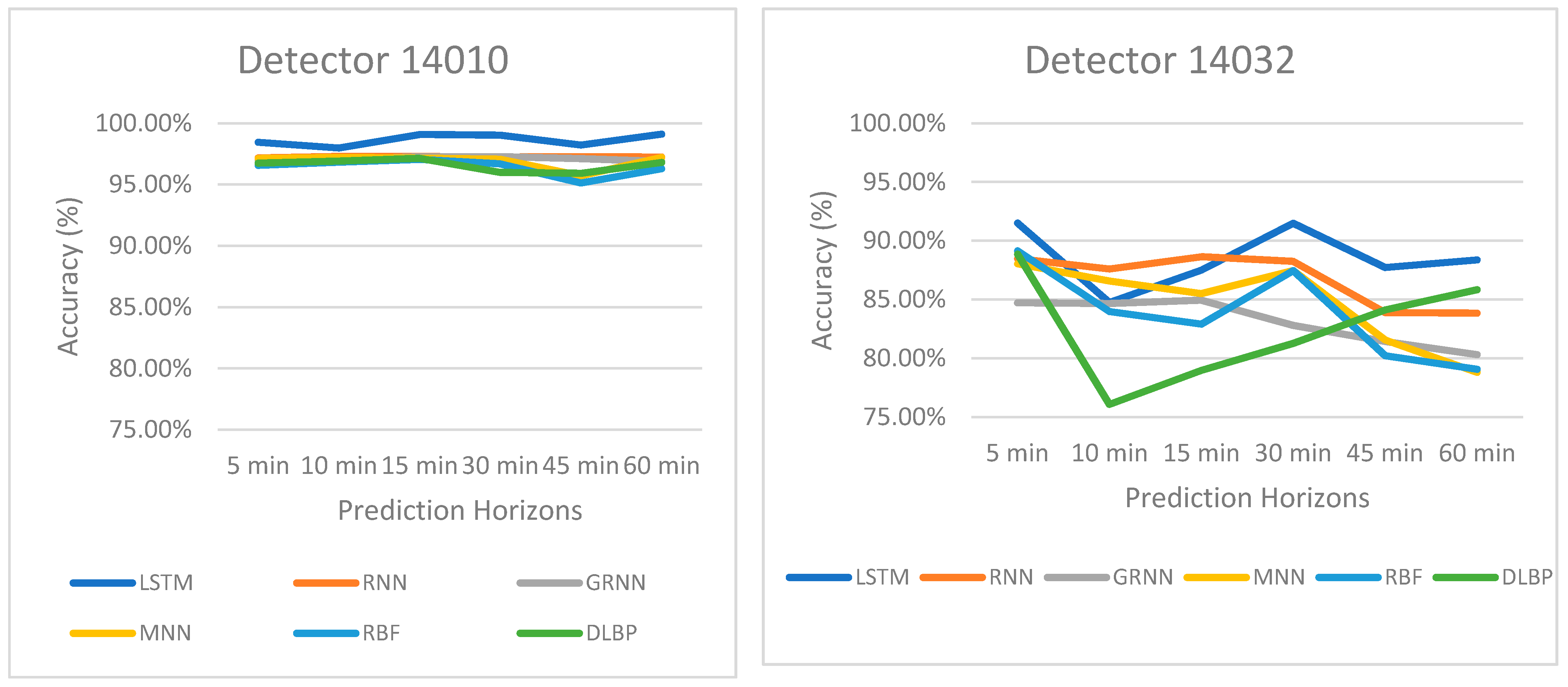
4.2.3. Eastbound Direction—Temporal Prediction Accuracies
The experimental results for the temporal variations in the eastbound direction are provided in Table 6 and Figure 9. The cells in the table that are highlighted in orange show the highest accuracies obtained, while the cells highlighted in green show the lowest. The results show that the LSTM generally has superior performance when compared to the RNN, GRNN, MNN, RBF and DLBP neural network.
Detector 14010 shows that the LSTM provides higher prediction accuracies of 98.44% for 5-min prediction horizons and 99.10% for 60-min horizons. For the LSTM, the accuracies do not deteriorate as the prediction horizon increases. For example, the accuracy is 97.97% for the 10-min horizon and remains steady at 99.10% for 60-min prediction horizons. This shows the ability of the system to capture the complexity of a longer speed prediction horizon. For the eastbound direction, the RBF had the least accurate predictions out of the six models.
For detector 14032, the results for the LSTM were the lowest compared to all detectors from WB and EB. This is maybe due to the data patterns for this detector which experienced heavy congestion at certain times during the months of July compared to other detectors. For 10-min horizons, the accuracy is 84.74% compared to 88.37% for the 60-min horizon. Also, it can be noted that the RNN provides better accuracy for 10-min and 15-min prediction horizons. However, the LSTM provides better accuracy overall for detector 14032. For short prediction, the GRNN and the DLBP neural network provided the least accurate predictions, while for longer prediction horizons (45 and 60 min), the RBF and MNN had the lowest performance of 80.21% and 78.80%, respectively.
For detector 14045, the LSTM outperforms all other 6 models with an accuracy ranging from 96.42% to 99.01%. The DLBP neural network, MNN and RBF provided the least accuracies for shorter prediction horizons up to 30 min, while the RBF had the lowest accuracy of 93.02% compared to 96.42% for the LSTM for 45-min horizons. The GRNN provided the least accurate predictions for 60-min horizons with 91.93% accuracy compared to 98.77% and 96.05 for the LSTM and RNN, respectively.
For detector 14061, the LSTM provided good accuracy for all time horizons ranging from 96.9% to 99.95%, except for the 60-min horizon where the RBF provided the highest accuracy of 96% compared to 93% for the LSTM. For 15-min horizons, the RBF achieved the lowest accuracy of 95.93% compared to the highest accuracy of 99.80% for the LSTM.
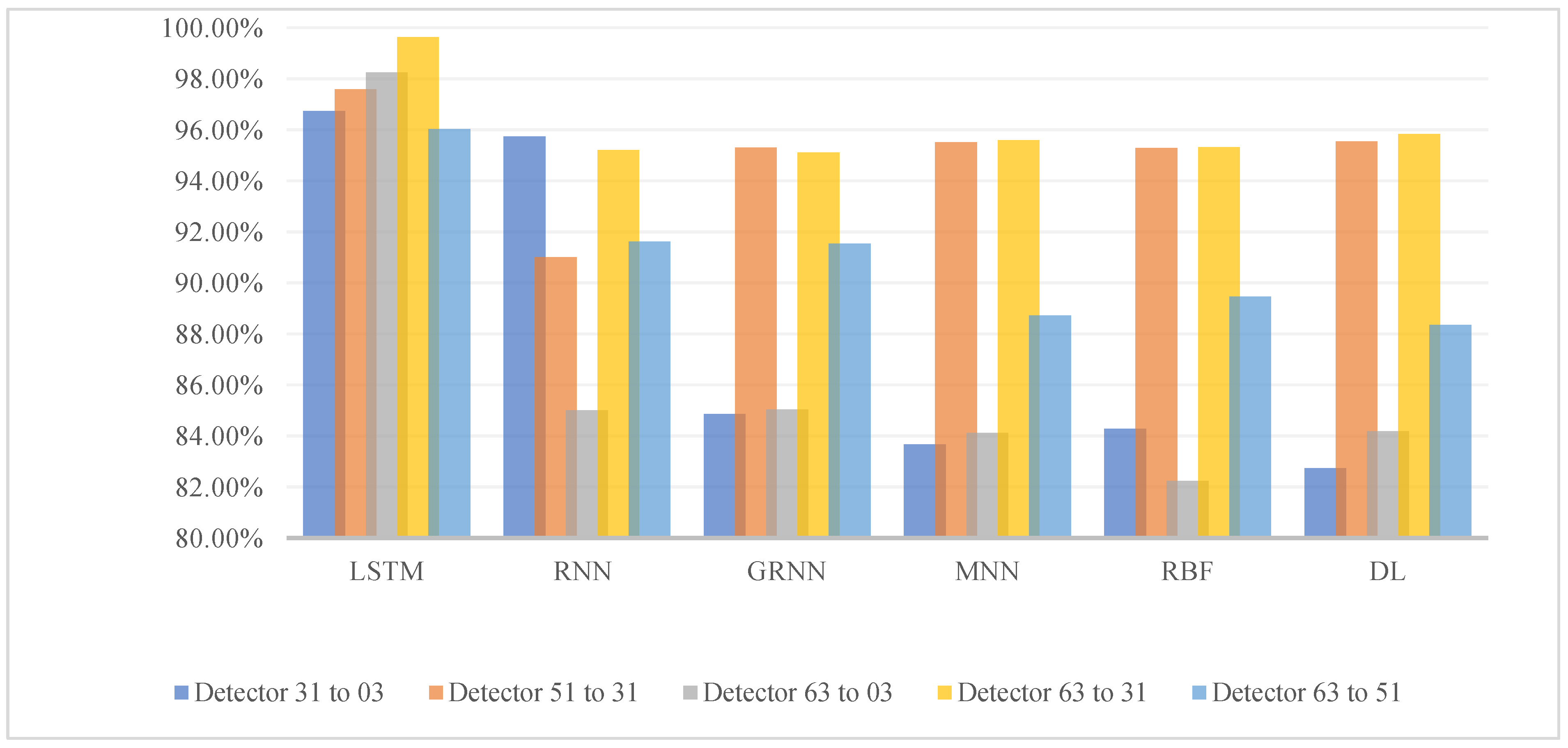
4.2.4. Eastbound Direction—Spatial Prediction Accuracies
For the eastbound direction, the results are similar for westbound reported before, where the accuracy of prediction is not affected as the distance changes. As can be seen in Table 7 and Figure 10, the LSTM provides the highest accuracy for most distance ranges, whereas the RNN provides the least accuracy. Overall, the LSTM provides the highest accuracy ranges for detectors that are furthest apart (15.45 km) with an accuracy result of 99.95%.
5. Conclusions and Future Directions
This paper developed and evaluated robust models for spatial and temporal predictions of traffic conditions at different locations on a real-world road facility in Melbourne, Australia. These models were developed using the Long Short-Term Memory (LSTM) network using a large data set of traffic observations, comprising 288,653 data points. The findings showed that the LSTM architecture provided the highest predictive intelligence accuracy for both temporal and spatial predictions. In particular, the models showed resilience as the prediction horizons increased spatially for distances up to 15 km and temporally up to 60 min providing a remarkable performance compared to the other architectures tested. Another important contribution of this work is demonstrating the feasibility of transferring a model which has been developed for one location for use at other multiple locations across the same facility, which is important for decision making when the input data of one location is missing or not available.
Future work will explore incorporating more inputs such as flow, occupancy as well as other important external factors such as weather to further refine the prediction models. In addition, more detector locations and spatial distributions along the entire road network will be utilised for future prediction analysis, including generation of new data sets for edge cases based on calibrated traffic simulation models and digital twins of the road facilities under consideration. Finally, future studies should also include additional advanced architectures and explore the influence of network parameters and sensitivity analyses of results.
Author Contributions
H.D., R.L.A.: planning, conceptualisation, and data collation. R.L.A., P.-W.T.: methodology, algorithm development and generation of results. H.D., R.L.A.: data analysis, pre-processing and curation. R.L.A., S.L.: drafting of paper content. R.L.A., S.L., and H.D.: writing, reviewing and editing. H.D.: supervision and mentoring of research students. All authors have read and agreed to the published version of the manuscript.
Funding
This research received no external funding.
Acknowledgments
This work was performed on the OzSTAR supercomputer national facility at the Swinburne University of Technology. The OzSTAR program receives funding in part from the Astronomy National Collaborative Research Infrastructure Strategy (NCRIS) allocation provided by the Australian Government. Also, the first author would like to acknowledge her PhD scholarship provided by the Iraqi Government and Swinburne University of Technology in Melbourne, Australia.
Conflicts of Interest
The authors declare no conflict of interest.
References
- Abduljabbar, R.; Dia, H.; Liyanage, S.; Bagloee, S.A. Applications of artificial intelligence in transport: An overview. Sustainability 2019, 11, 189. [Google Scholar] [CrossRef] [Green Version]
- Abduljabbar, R.; Dia, H. Predictive Intelligence: A Neural Network Learning System for Traffic Condition Prediction and Monitoring on Freeways. J. East. Asia Soc. Transp. Stud. 2019, 13, 1785–1800. [Google Scholar]
- Mahamuni, A. Internet of Things, machine learning, and artificial intelligence in the modern supply chain and transportation. Def. Transp. J. 2018, 74, 14–17. [Google Scholar]
- Barceló, J. Fundamentals of Traffic Simulation; Springer: Berlin/Heidelberg, Germany, 2010. [Google Scholar]
- Papageorgiou, M.; Kiakaki, C.; Dinopoulou, V.; Kotsialos, A.; Wang, Y. Review of road traffic control strategies. Proc. IEEE 2003, 91, 2043–2067. [Google Scholar] [CrossRef] [Green Version]
- Abduljabbar, R.; Dia, H. A Deep Learning Approach for Freeway Vehicle Speed and Flow Prediction; Australasian Transport Research Forum: Canberra, Australia, 2019. [Google Scholar]
- Song, Z.; Guo, Y.; Wu, Y.; Ma, J. Short-term traffic speed prediction under different data collection time intervals using a SARIMA-SDGM hybrid prediction model. PLoS ONE 2019, 14, e0218626. [Google Scholar] [CrossRef]
- Jiang, B.; Fei, Y. Vehicle Speed Prediction by Two-Level Data Driven Models in Vehicular Networks. IEEE Trans. Intell. Transp. Syst. 2016, 18, 1793–1801. [Google Scholar] [CrossRef]
- Vlahogianni, E.I.; Karlaftis, M.G.; Golias, J.C. Short-term traffic forecasting: Where we are and where we’re going. Transp. Res. Part C Emerg. Technol. 2014, 43, 3–19. [Google Scholar] [CrossRef]
- Lund, R. Time Series Analysis and Its Applications: With R Examples Robert H. Shumway and David S. Stoffer. J. Am. Stat. Assoc. 2007, 102, 1079. [Google Scholar] [CrossRef]
- Ma, X.; Tao, Z.; Wang, Y.; Yu, H.; Wang, Y. Long short-term memory neural network for traffic speed prediction using remote microwave sensor data. Transp. Res. Part. C Emerg. Technol. 2015, 54, 187–197. [Google Scholar] [CrossRef]
- van Hinsbergen, C.; van Lint, J.; van Zuylen, H. Bayesian committee of neural networks to predict travel times with confidence intervals. Transp. Res. Part. C Emerg. Technol. 2009, 17, 498–509. [Google Scholar] [CrossRef]
- Karlaftis, M.G.; Vlahogianni, E.I. Memory properties and fractional integration in transportation time-series. Transp. Res. Part C Emerg. Technol. 2009, 17, 444–453. [Google Scholar] [CrossRef]
- Fusco, G.; Colombaroni, C.; Isaenko, N. Short-term speed predictions exploiting big data on large urban road networks. Transp. Res. Part C Emerg. Technol. 2016, 73, 183–201. [Google Scholar] [CrossRef]
- Ross, P. Exponential Filtering of Traffic Data; Transportation Research Board: Washington, DC, USA, 1982. [Google Scholar]
- Chan, K.Y.; Dillon, T.S.; Singh, J.; Chang, E. Neural-Network-Based Models for Short-Term Traffic Flow Forecasting Using a Hybrid Exponential Smoothing and Levenberg–Marquardt Algorithm. IEEE Trans. Intell. Transp. Syst. 2012, 13, 644–654. [Google Scholar] [CrossRef]
- Guo, J.; Huang, W.; Williams, B.M. Adaptive Kalman filter approach for stochastic short-term traffic flow rate prediction and uncertainty quantification. Transp. Res. Part C Emerg. Technol. 2014, 43, 50–64. [Google Scholar] [CrossRef]
- Lippi, M.; Bertini, M.; Frasconi, P. Short-Term Traffic Flow Forecasting: An Experimental Comparison of Time-Series Analysis and Supervised Learning. IEEE Trans. Intell. Transp. Syst. 2013, 14, 871–882. [Google Scholar] [CrossRef]
- Ahmed, M.S.; Cook, A.R. Analysis of Freeway Traffic Time-Series Data by Using Box-Jenkins Techniques; Transportation Research Board: Washington, DC, USA, 1979. [Google Scholar]
- Chen, C.; Hu, J.; Meng, Q.; Zhang, Y. Short-time traffic flow prediction with ARIMA-GARCH model. In 2011 IEEE Intelligent Vehicles Symposium (IV); IEEE: New York, NY, USA, 2011; pp. 607–612. [Google Scholar]
- Ding, Q.Y.; Wang, X.F.; Zhang, X.Y.; Sun, Z.Q. Forecasting Traffic Volume with Space-Time ARIMA Model. Adv. Mater. Res. 2010, 156–157, 979–983. [Google Scholar] [CrossRef]
- Zahid, M.; Chen, Y.; Jamal, A.; Mamadou, C.Z. Freeway Short-Term Travel Speed Prediction Based on Data Collection Time-Horizons: A Fast Forest Quantile Regression Approach. Sustainability 2020, 12, 646. [Google Scholar] [CrossRef] [Green Version]
- Gu, Y.; Lu, W.; Qin, L.; Li, M.; Shao, Z. Short-term prediction of lane-level traffic speeds: A fusion deep learning model. Transp. Res. Part C Emerg. Technol. 2019, 106, 1–16. [Google Scholar] [CrossRef]
- Karlaftis, M.; Vlahogianni, E. Statistical methods versus neural networks in transportation research: Differences, similarities and some insights. Transp. Res. Part C Emerg. Technol. 2011, 19, 387–399. [Google Scholar] [CrossRef]
- Castro-Neto, M.; Jeong, Y.-S.; Jeong, M.-K.; Han, L.D. Online-SVR for short-term traffic flow prediction under typical and atypical traffic conditions. Expert Syst. Appl. 2009, 36, 6164–6173. [Google Scholar] [CrossRef]
- Vanajakshi, L.; Rilett, L.R. Support Vector Machine Technique for the Short Term Prediction of Travel Time. In Proceedings of the 2007 IEEE Intelligent Vehicles Symposium, Istanbul, Turkey, 13–15 June 2007; pp. 600–605. [Google Scholar]
- Wang, J.; Shi, Q. Short-term traffic speed forecasting hybrid model based on Chaos–Wavelet Analysis-Support Vector Machine theory. Transp. Res. Part C Emerg. Technol. 2013, 27, 219–232. [Google Scholar] [CrossRef]
- Laña, I.; Lobo, J.L.; Capecci, E.; Del Ser, J.; Kasabov, N. Adaptive long-term traffic state estimation with evolving spiking neural networks. Transp. Res. Par. C Emerg. Technol. 2019, 101, 126–144. [Google Scholar] [CrossRef]
- Li, L.; Qin, L.; Qu, X.; Zhang, J.; Wang, Y.; Ran, B. Day-ahead traffic flow forecasting based on a deep belief network optimised by the multi-objective particle swarm algorithm. Knowl. Based Syst. 2019, 172, 1–14. [Google Scholar] [CrossRef]
- Lefevre, S.; Sun, C.; Bajcsy, R.; Laugier, C. Comparison of parametric and non-parametric approaches for vehicle speed prediction. In Proceedings of the 2014 American Control Conference, Portland, OR, USA, 4–6 June 2014; pp. 3494–3499. [Google Scholar]
- Sun, C.; Hu, X.; Moura, S.J.; Sun, F. Velocity Predictors for Predictive Energy Management in Hybrid Electric Vehicles. IEEE Trans. Control. Syst. Technol. 2014, 23, 1197–1204. [Google Scholar] [CrossRef]
- Vlahogianni, E.I.; Golias, J.C.; Karlaftis, M.G. Short-term traffic forecasting: Overview of objectives and methods. Transp. Rev. 2004, 24, 533–557. [Google Scholar] [CrossRef]
- Smith, B.L.; Demetsky, M.J. Short-term traffic flow prediction models-a comparison of neural network and non-parametric regression approaches. In Proceedings of the IEEE International Conference on Systems, Man and Cybernetics, San Antonio, TX, USA, 2–5 October 1994; Volume 2, pp. 1706–1709. [Google Scholar]
- Guo, J.; Luo, Y.; Li, K. Adaptive neural-network sliding mode cascade architecture of longitudinal tracking control for unmanned vehicles. Nonlinear Dyn. 2016, 87, 2497–2510. [Google Scholar] [CrossRef]
- Kuang, X.; Xu, L.; Huang, Y.; Liu, F. Real-time forecasting for short-term traffic flow based on General Regression Neural Network. In Proceedings of the 2010 8th World Congress on Intelligent Control and Automation, Jinan, China, 7–9 July 2010; pp. 2776–2780. [Google Scholar] [CrossRef]
- Morton, J.; Wheeler, T.A.; Kochenderfer, M.J. Analysis of Recurrent Neural Networks for Probabilistic Modeling of Driver Behavior. IEEE Trans. Intell. Transp. Syst. 2017, 18, 1289–1298. [Google Scholar] [CrossRef]
- Gers, F.A.; Schmidhuber, J.; Cummins, F. Learning to Forget: Continual Prediction with LSTM. Neural Comput. 2000, 12, 2451–2471. [Google Scholar] [CrossRef]
- Yeon, K.; Min, K.; Shin, J.; Sunwoo, M.; Han, M. Ego-Vehicle Speed Prediction Using a Long Short-Term Memory Based Recurrent Neural Network. Int. J. Automot. Technol. 2019, 20, 713–722. [Google Scholar] [CrossRef]
- Yu, H.; Wu, Z.; Wang, S.; Wang, Y.; Ma, X. Spatiotemporal Recurrent Convolutional Networks for Traffic Prediction in Transportation Networks. Sensors 2017, 17, 1501. [Google Scholar] [CrossRef] [Green Version]
- Ma, X.; Dai, Z.; He, Z.; Ma, J.; Wang, Y.; Wang, Y. Learning Traffic as Images: A Deep Convolutional Neural Network for Large-Scale Transportation Network Speed Prediction. Sensors 2017, 17, 818. [Google Scholar] [CrossRef] [PubMed] [Green Version]
- Vlahogianni, E.I.; Karlaftis, M.G.; Golias, J.C. Spatio-temporal short-term urban traffic volume forecasting using genetically optimised modular networks. Comput. Aided Civ. Infrastruct. Eng. 2007, 22, 317–325. [Google Scholar] [CrossRef]
- Cigizoglu, H.K. Generalised regression neural network in monthly flow forecasting. Civ. Eng. Environ. Syst. 2005, 22, 71–81. [Google Scholar] [CrossRef]
- Matlab. Long Short-Term Memory Networks. Available online: https://au.mathworks.com/help/deeplearning/ug/long-short-term-memory-networks.html (accessed on 9 February 2020).
- Google Maps. 2020. Eastern Freeway, Google Maps, Accessed 31 August 2019. Available online: https://www.google.com/maps/place/Eastern+Fwy,+Melbourne+VIC/@-37.7894853,145.0653246,8233m/data=!3m1!1e3!4m5!3m4!1s0x6ad646cddfc42b73:0x1d8fc4fc43bf7971!8m2!3d-37.7820449!4d145.0746107 (accessed on 9 February 2020).
- NeuralWare. NeuralWare Neural Computing, Using NeuralWorks, and Reference GuideNeuralWare, Pittsburgh, PA. Available online: www.neuralware.com (accessed on 9 February 2020).
- Dia, H.; Rose, G.; Snell, A. Comparative Performance of Freeway Automated Incident Detection Algorithms; Institute of Transport Studies: Monash, Australia, 1996. [Google Scholar]
- Dia, H.; Rose, G. Development of artificial neural network models for automated detection of freeway incidents. In Proceedings of the 7th World Conference on Transport Research, Sydney, Australia, 16–22 July 1995; Volume 2. [Google Scholar]
- Thomas, K.; Dia, H.; Cottman, N. Simulation of arterial incident detection using neural networks. In Proceedings of the 8th World Congress on Intelligent Transport Systems, Sydney, Australia, 30 September–4 October 2001. [Google Scholar]
- Sutandi, C.; Dia, H. Performance Evaluation of an Advanced Traffic Control System in a Developing Country. In Proceedings of the 6th EASTS Conference, Bangkok, Thailand, 21–24 September 2005. [Google Scholar]
- Nigarnjanagoo, S.; Dia, H. Evaluation of a Dynamic Signal Optimisation Control Model using Traffic Simulation. Special Issue on the Computerisation of Transportation: Sophisticated Systems Incorporating IT in the Mobility of People and Goods. J. Int. Assoc. Traffic Saf. Sci. 2005, 29, 22–30. [Google Scholar]
- Dia, H.; Harney, D.; Boyle, A. Dynamics of drivers’ route choice decisions under advanced traveller information systems. In Roads and Transport Research; ARRB Transport Research Ltd: Vermont South, Victoria, Australia, 2001; Volume 10, pp. 2–12. [Google Scholar]
- Thomas, K.; Dia, H. Comparative evaluation of freeway incident detection models using field data. IEE Proc. Intell. Transp. Syst. 2006, 153, 230. [Google Scholar] [CrossRef]
- Panwai, S.; Dia, H. Development and Evaluation of a Reactive Agent-Based Car Following Model. In Proceedings of the Intelligent Vehicles and Road Infrastructure Conference (IVRI ’05), Melbourne, Australia, 16–17 February 2005. [Google Scholar]
- Smit, R.; Dia, H.; Morawska, L. Road Traffic Emission and Fuel Consumption Modelling: Trends, New Developments and Future Challenges. In Traffic Related Air Pollution; Demidov, S., Bonnet, J., Eds.; Nova Science Publishers: Hauppauge, NY, USA, 2005; pp. 29–68. [Google Scholar]
- Hochreiter, S.; Schmidhuber, J. Long Short-Term Memory. Neural Comput. 1997, 9, 1735–1780. [Google Scholar] [CrossRef] [PubMed]
Figure 1.
Spatio-temporal modelling process for eastbound (EB) and westbound (WB) detectors.

Figure 2.
Long Short-Term Memory (LSTM) architecture [42].
Figure 2.
Long Short-Term Memory (LSTM) architecture [42].

Figure 3.
Detector locations on the mainstream of Eastern Freeway eastbound (EB) and westbound (WB) [44].
Figure 3.
Detector locations on the mainstream of Eastern Freeway eastbound (EB) and westbound (WB) [44].

Figure 4.
Eastern Freeway section and location of detectors.

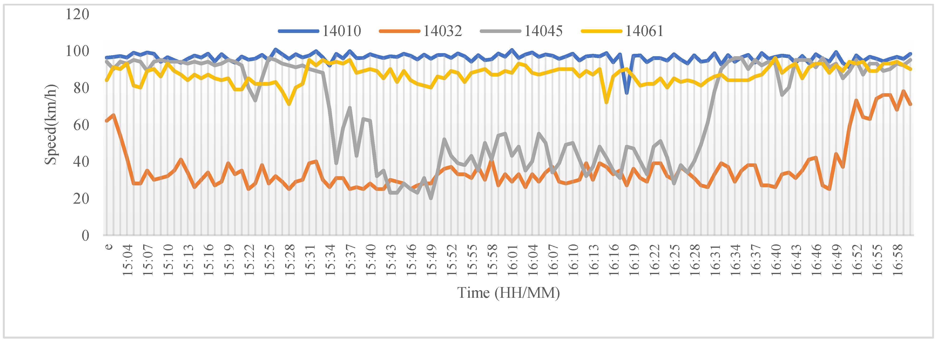
Figure 5.
Sample speed data pattern for eastbound detectors.

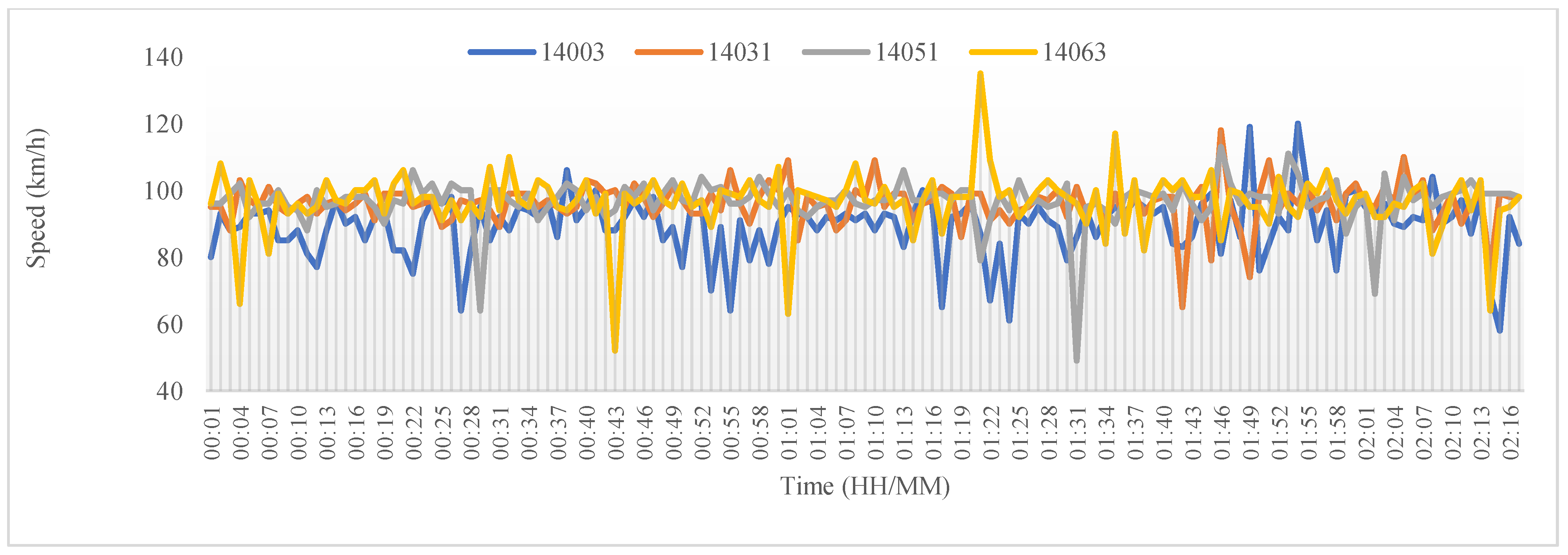
Figure 6.
Sample speed data pattern for westbound detectors.

Figure 7.
Comparison of temporal results for westbound.

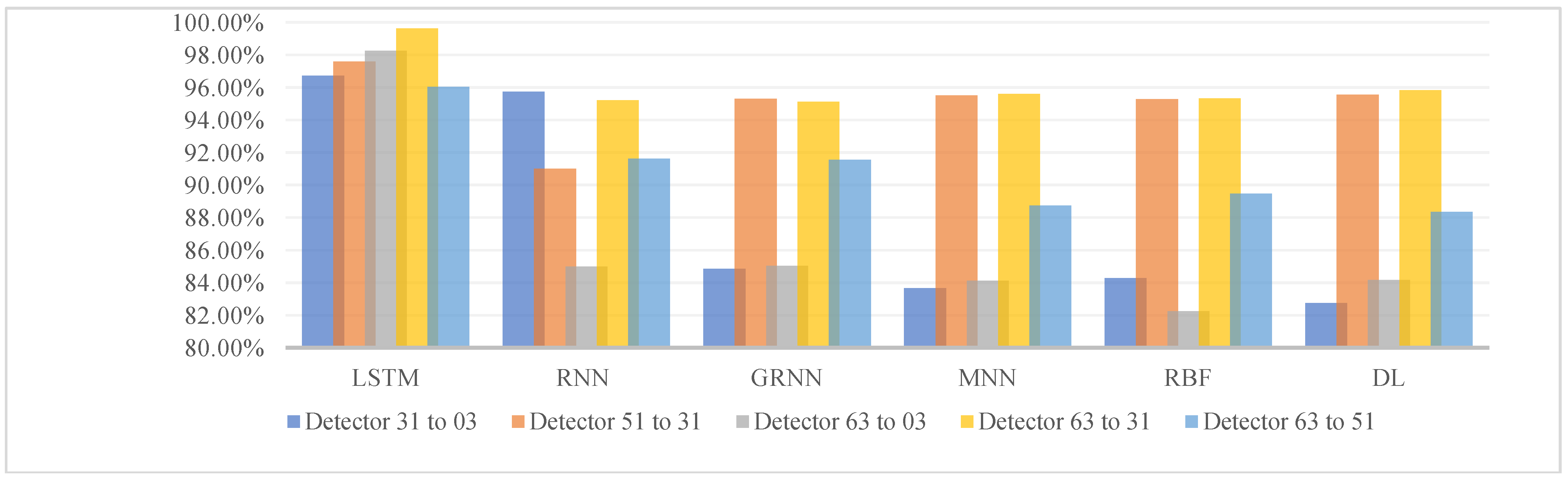
Figure 8.
Graphical representation of spatial prediction results for the westbound direction.

Figure 9.
Comparison of temporal results for the eastbound direction.


Figure 10.
Graphical representation of spatial prediction results for the eastbound direction.


Table 1.
Model Parameters.
| Parameters | Settings |
|---|---|
| Gradient Decay Factor | 0.9 |
| Initial Learning Rate | 0.005 |
| Minimum Batch Size | 128 |
| Maximum Epochs | 300 |
| Training Optimizer | adaptive moment estimation optimiser |
| Dropping Learning Rate During Training | piecewise |
| Learning Rate Drop Period | 125 |
| Factor for Learning Rate Dropping | 0.2 |
Table 2.
Description of detector locations on the Eastern Freeway.
| No | Detection Name | X | Y | No. of Lanes | Location |
|---|---|---|---|---|---|
| 1 | 14010 EB | 145.017 | −37.791 | 5 | Eastern Freeway West of Yarra River OB |
| 2 | 14032 EB | 145.083 | −37.783 | 3 | Eastern Freeway Thompsons Road East Outbound |
| 3 | 14045 EB | 145.122 | −37.78 | 3 | Eastern Freeway between Elgar and Tram Road |
| 4 | 14061 EB | 145.168 | −37.803 | 3 | Eastern Freeway OB between Springvale and Blackburn Roads |
| 5 | 14003 WB | 145.002 | −37.795 | 5 | Eastern Freeway Merri Creek East Inbound |
| 6 | 14031 WB | 145.08 | −37.78 | 3 | Eastern Freeway Bulleen Road East Inbound |
| 7 | 14051 WB | 145.139 | −37.798 | 4 | Eastern Freeway west of Middleborough Road IB |
| 8 | 14063 WB | 145.174 | −37.804 | 3 | Eastern Freeway west of Springvale Road |
Table 3.
Speed datasets used for each detector in two travel directions.
| Travel Direction | Detector | Total Speed Data Set | Training Data Set | Test and Validation Set |
|---|---|---|---|---|
| Eastbound | 14010 EB | 22,781 | 13,669 | 9112 |
| 14032 EB | 38,808 | 23,285 | 15,523 | |
| 14045 EB | 40,403 | 24,242 | 16,161 | |
| 14061 EB | 41,135 | 24,681 | 16,454 | |
| Westbound | 14063 WB | 39,914 | 23,948 | 15,966 |
| 14051 WB | 39,410 | 23,646 | 15,764 | |
| 14031 WB | 38,246 | 22,948 | 15,298 | |
| 14003 WB | 27,956 | 16,774 | 11,182 | |
| Total | - | 288,653 | 173,193 | 115,460 |
Table 4.
Temporal prediction accuracies for westbound detectors.
| Detector | Prediction Horizon | LSTM | RNN | GRNN | MNN | RBF | DLBP |
|---|---|---|---|---|---|---|---|
| Detector 14003 | 5 min | 94.24% | 92.91% | 93.01% | 93.58% | 93.85% | 93.72% |
| 10 min | 94.04% | 92.23% | 92.23% | 93.19% | 93.04% | 90.31% | |
| 15 min | 99.02% | 91.51% | 91.03% | 93.24% | 91.97% | 89.68% | |
| 30 min | 96.86% | 88.93% | 87.80% | 86.67% | 89.53% | 89.44% | |
| 45 min | 95.05% | 86.76% | 87.88% | 86.10% | 86.57% | 88.00% | |
| 60 min | 94.97% | 86.76% | 86.25% | 84.12% | 85.39% | 85.88% | |
| Detector 14031 | 5 min | 95.23% | 96.54% | 96.05% | 96.78% | 96.54% | 96.41% |
| 10 min | 97.55% | 96.50% | 96.06% | 96.14% | 96.20% | 96.62% | |
| 15 min | 96.65% | 96.28% | 96.05% | 96.58% | 96.67% | 96.36% | |
| 30 min | 95.65% | 96.17% | 96.06% | 96.51% | 96.27% | 93.89% | |
| 45 min | 95.54% | 95.60% | 96.05% | 95.65% | 96.09% | 96.32% | |
| 60 min | 98.96% | 95.51% | 96.01% | 96.26% | 95.93% | 95.22% | |
| Detector 14051 | 5 min | 98.47% | 95.01% | 95.51% | 95.17% | 94.71% | 94.14% |
| 10 min | 95.61% | 94.55% | 95.03% | 94.89% | 94.83% | 95.05% | |
| 15 min | 96.31% | 93.51% | 94.31% | 94.22% | 93.99% | 94.65% | |
| 30 min | 97.41% | 91.92% | 92.68% | 93.77% | 92.75% | 92.42% | |
| 45 min | 99.94% | 89.86% | 92.38% | 89.72% | 91.50% | 91.65% | |
| 60 min | 99.43% | 83.16% | 92.37% | 92.01% | 91.57% | 88.34% | |
| Detector 14063 | 5 min | 98.66% | 94.10% | 94.71% | 92.89% | 94.33% | 90.23% |
| 10 min | 98.76% | 94.06% | 94.43% | 94.12% | 93.39% | 93.62% | |
| 15 min | 97.68% | 93.81% | 93.91% | 93.81% | 92.33% | 92.00% | |
| 30 min | 98.75% | 93.52% | 93.46% | 93.65% | 92.86% | 82.29% | |
| 45 min | 98.22% | 93.39% | 93.35% | 93.00% | 92.45% | 92.24% | |
| 60 min | 98.77% | 93.38% | 93.32% | 92.71% | 91.77% | 91.83% |
Table 5.
Spatial prediction accuracies for westbound detectors.
| Detectors | Detector 63 to 51 | Detector 51 to 31 | Detector 31 to 03 | Detector 63 to 31 | Detector 63 to 03 |
|---|---|---|---|---|---|
| Spatial Distance | 5.4 km | 6.1 km | 7.1 km | 11.5 km | 18.6 km |
| LSTM | 96.03% | 97.59% | 96.73% | 99.63% | 98.24% |
| RNN | 91.61% | 91.00% | 95.74% | 95.21% | 85.00% |
| GRNN | 91.54% | 95.31% | 84.85% | 95.11% | 85.04% |
| MNN | 88.72% | 95.52% | 83.67% | 95.60% | 84.11% |
| RBF | 89.46% | 84.28% | 95.28% | 82.24% | 89.46% |
| DLBP | 88.34% | 82.74% | 95.55% | 84.18% | 88.34% |
Table 6.
Temporal prediction accuracies for eastbound detectors.
| Detector | Prediction Horizon | LSTM | RNN | GRNN | MNN | RBF | DLBP |
|---|---|---|---|---|---|---|---|
| Detector 14010 | 5 min | 98.44% | 97.16% | 97.01% | 97.11% | 96.56% | 96.74% |
| 10 min | 97.97% | 97.28% | 97.00% | 97.21% | 96.81% | 96.90% | |
| 15 min | 99.07% | 97.28% | 97.27% | 97.14% | 97.04% | 97.13% | |
| 30 min | 99.01% | 97.24% | 97.27% | 97.06% | 96.68% | 95.99% | |
| 45 min | 98.22% | 97.25% | 97.10% | 95.71% | 95.12% | 95.90% | |
| 60 min | 99.10% | 97.24% | 96.87% | 97.20% | 96.29% | 96.80% | |
| Detector 14032 | 5 min | 91.50% | 88.48% | 84.72% | 88.03% | 89.14% | 88.86% |
| 10 min | 84.74% | 87.59% | 84.66% | 86.57% | 83.97% | 76.08% | |
| 15 min | 87.50% | 88.63% | 84.94% | 85.50% | 82.91% | 78.98% | |
| 30 min | 91.48% | 88.24% | 82.80% | 87.46% | 87.46% | 81.27% | |
| 45 min | 87.72% | 83.88% | 81.42% | 81.55% | 80.21% | 84.12% | |
| 60 min | 88.37% | 83.84% | 80.31% | 78.80% | 79.07% | 85.84% | |
| Detector 14045 | 5 min | 99.01% | 96.69% | 95.99% | 95.18% | 95.80% | 92.79% |
| 10 min | 97.31% | 96.44% | 95.95% | 96.18% | 95.10% | 92.56% | |
| 15 min | 98.76% | 96.30% | 95.94% | 96.37% | 93.70% | 92.52% | |
| 30 min | 98.81% | 96.26% | 95.81% | 94.19% | 95.59% | 96.32% | |
| 45 min | 96.42% | 96.15% | 95.70% | 94.29% | 93.02% | 95.98% | |
| 60 min | 98.77% | 96.05% | 91.39% | 93.64% | 95.10% | 95.60% | |
| Detector 14061 | 5 min | 99.95% | 96.44% | 96.02% | 96.39% | 96.17% | 96.31% |
| 10 min | 99.96% | 96.44% | 96.02% | 96.23% | 96.34% | 95.64% | |
| 15 min | 99.80% | 96.40% | 96.01% | 96.34% | 95.93% | 96.26% | |
| 30 min | 96.90% | 96.35% | 95.99% | 96.05% | 95.81% | 95.27% | |
| 45 min | 97.04% | 96.13% | 95.99% | 95.91% | 96.25% | 94.46% | |
| 60 min | 93.00% | 95.80% | 95.97% | 95.78% | 96.14% | 95.90% |
Table 7.
Spatial prediction accuracies for eastbound detectors.
| Detectors | Detector 45 to 61 | Detector 32 to 45 | Detector 10 to 32 | Detector 10 to 45 | Detector 10 to 61 |
|---|---|---|---|---|---|
| Location between Detectors | 4.1 km | 5.4 km | 5.95 km | 11.35 km | 15.45 km |
| LSTM | 98.49% | 99.15% | 81.00% | 96.95% | 99.95% |
| RNN | 96% | 94.97% | 81.00% | 95.64% | 94.04% |
| GRNN | 95.83% | 92.61% | 83.04% | 88.85% | 95.63% |
| MNN | 95.61% | 93.68% | 82.40% | 92.64% | 95.89% |
| RBF | 95.66% | 94.26% | 81.64% | 93.02% | 94.33% |
| DL | 95.48% | 95.29% | 82.73% | 91.97% | 95.47% |
Publisher’s Note: MDPI stays neutral with regard to jurisdictional claims in published maps and institutional affiliations. |
© 2021 by the authors. Licensee MDPI, Basel, Switzerland. This article is an open access article distributed under the terms and conditions of the Creative Commons Attribution (CC BY) license (http://creativecommons.org/licenses/by/4.0/).
Share and Cite
MDPI and ACS Style
Abduljabbar, R.L.; Dia, H.; Tsai, P.-W.; Liyanage, S. Short-Term Traffic Forecasting: An LSTM Network for Spatial-Temporal Speed Prediction. Future Transp. 2021, 1, 21-37. https://0-doi-org.brum.beds.ac.uk/10.3390/futuretransp1010003
AMA Style
Abduljabbar RL, Dia H, Tsai P-W, Liyanage S. Short-Term Traffic Forecasting: An LSTM Network for Spatial-Temporal Speed Prediction. Future Transportation. 2021; 1(1):21-37. https://0-doi-org.brum.beds.ac.uk/10.3390/futuretransp1010003
Chicago/Turabian StyleAbduljabbar, Rusul L., Hussein Dia, Pei-Wei Tsai, and Sohani Liyanage. 2021. "Short-Term Traffic Forecasting: An LSTM Network for Spatial-Temporal Speed Prediction" Future Transportation 1, no. 1: 21-37. https://0-doi-org.brum.beds.ac.uk/10.3390/futuretransp1010003