
Conductive Heat Transfer in Thermal Bridges


Mathias Fuchs Services, Hallgartenstr. 6, 81375 Munich, Germany
Encyclopedia 2022, 2(2), 1019-1035; https://0-doi-org.brum.beds.ac.uk/10.3390/encyclopedia2020067
Submission received: 4 April 2022
/
Revised: 19 May 2022
/
Accepted: 20 May 2022
/
Published: 24 May 2022
(This article belongs to the Collection Encyclopedia of ZEMCH Research and Development)
Definition
:A thermal bridge is a component of a building that is characterized by a higher thermal loss compared with its surroundings. Their accurate modeling is a key step in energy performance analysis due to the increased awareness of the importance of sustainable design. Thermal modeling in architecture and engineering is often not carried out volumetrically, thereby sacrificing accuracy for complex geometries, whereas numerical textbooks often give the finite element method in much higher generality than required, or only treat the case of uniform materials. Despite thermal modeling traditionally belonging exclusively to the engineer’s toolbox, computational and parametric design can often benefit from understanding the key steps of finite element thermal modeling, in order to inform a real-time design feedback loop. In this entry, these gaps are filled and the reader is introduced to all relevant physical and computational notions and methods necessary to understand and compute the stationary energy dissipation and thermal conductance of thermal bridges composed of materials in complex geometries. The overview is a self-contained and coherent expository, and both physically and mathematically as correct as possible, but intuitive and accessible to all audiences. Details for a typical example of an insulated I-beam thermal bridge are provided.
1. Introduction
Building energy performance simulation, modeling and optimization has become an ever more important discipline at the multidisciplinary junction between building physics, design, architecture, engineering, numerical mathematics and optimization. Soaring energy costs and an increased awareness of the urgency of sustainability amid a global energy crisis have led to growing interest far beyond the original scope of an engineering sub-discipline. Physically, heat transfer is described by the heat equation—a century old and well studied partial differential equation (henceforth abbreviated PDE). In principle, it determines the heat distribution in a given geometry, for given material constants and boundary conditions, either in a time-dependent or time-independent manner. In practice, however, an accurate solution requires a finite element discretization of the heat equation. A finite element solution solves an approximation to the heat equation on a tetrahedralization of the input domain; see Zienkiewicz et al. [1] for a general introduction to finite element (FE) methods; Ciarlet [2] for an introduction to FE on the particular class of elliptic PDEs relevant here, and Wilson and Nickell [3], Lewis et al. [4] for the application of FE to thermal modeling. Effectively, this places simulation and modeling at the heart of every modern building performance simulation.
There is no treatment in the literature that coherently covers the engineering aspects together with the full three-dimensional FE method in a way that is accessible to an audience from, say, a design background. Most expositions focus either on basic one-dimensional quantities such as the U-value [5], on numerical methods for the full 3D heat transfer, or on computational design in view of architectural and artistic aspects [6]. A thermal bridge is defined as a building component with particularly high thermal loss; as such, they are the most important objects of modeling [7,8]. This entry aims to outline a complete introduction to put the reader in a position to understand all steps necessary to compute the energy loss incurred by a particular thermal bridge situation in design.
As a rule of thumb, heating costs constitute one of the largest shares of the per capita energy profile of the average Western inhabitant of moderate latitudes. For example, it is estimated that the entire average annual primary energy consumption in developed countries is roughly 100–200 GJ per capita [9]. On the other hand, for example in Germany, the annual per capita heating energy profile is estimated to be more than 3000 kWh ≈ 10 GJ per year [10]. Thus, a considerable fraction of about 5–10 percent of the energy is spent on heating alone. This places the heating energy profile among the top private household budget items.
Consequently, there are plenty of legal incentives, policies and regulations aimed at instigating energy efficiency certifications in most countries in the middle latitudes. Energy certification, consulting, contracting, and modernization have all become their own industry segments. This increased pressure on home owners, real estate agents and developers has recently led to the previously unthinkable situation where the energy certificate has the highest or one of the highest impacts on a real estate’s (rental) value, among all value predictors [11].
Apart from these environmental and monetary incentives for having good insulation, thermal performance and insulation are, of course, highly relevant in regards to building safety due to their importance for vapor condensation and mold prevention. Consequently, estimating and optimizing a building’s energy performance has become one of the cornerstones of sustainable architecture, modernization, renovation, maintenance and building safety.
There is an abundance of commercial and non-commercial FE software packages available on the market. It would seem difficult to even attempt to cite a comprehensive list of the most important ones, due to the far-reaching impact they have, the multitude of application scenarios, and the long amount of time these packages have already been under development for. For example, one of the most popular commercial software packages capable of modeling thermal conductance is ANSYS [12], and one of the most popular open source software packages if Freefem++ [13]. However, it is often desirable to understand and implement a basic FE algorithm from scratch, rather than treating the FE method as a black box. This entry aims to introduce students of all the aforementioned disciplines, in particular those without prior exposure to FE methods and computational physics from scratch to a state where the reader could, at least in principle, implement their own FE solution. In this text, no prior exposure to computational design, programming, or mathematics beyond an early undergraduate level are assumed. In particular, it will be explained how the seemingly arcane physical description of heat transfer translates into an amenable pseudo-code which can readily be employed and adapted to more specialized optimization questions.
Most architecturally inspired texts, or even those for engineering students, tend not to describe the full volumetric heat equation, and focus on one or two-dimensional case studies [14], or even just a description of insulation indicators such as U-values, avoiding differential equations altogether. On the other hand, mathematically oriented textbooks tend to ignore materials altogether, and just treat the “heat equation” in the form of where u is the temperature distribution and is a heat source term, is the time derivative, and is the Laplacian [15]. However, the relevant equation for use in our case is when is the steady state or stationary property and . In fact, there is usually no heating inside the thermal bridge. In contrast, the term needs to be replaced with the slightly more general expression . In this entry, the following convention is used: The operator ∇ applied to a scalar field such as u is the gradient of the scalar field, such as the temperature gradient, and ∇ applied to a vector field, such as the heat flux, is the divergence of the vector field. The reader is invited to recall that the divergence of a vector field is a scalar field that describes how much the vector field converges or diverges.
These variations of the heat equation will be explained in Section 3.2. For the purely mathematical and theoretical treatment, omitting from the picture makes almost no difference, but here, all the material properties are expressed through, and have an impact on the modeling, in terms of their conductivity . All of the information about the materials is in the quantity . It is isotropic but also non-uniform and hence can not be “pulled in front” as a simple constant number. Therefore, one can not simplify the term to as almost all mathematically oriented textbooks tend to do.
In this sense, the PDE literature equation is both an oversimplification of material continuity and a complication of time dependence. Due to these small differences, the classical PDE literature is almost useless for the architect and engineer who focuses on modeling thermal bridges. The passage from the PDE to the PDE —Equation (2) below—makes both the analytical understanding and the practical numerical treatment much easier to comprehend, but it is quite different and not entirely trivial.
Similarly, there do not seem to be many treatments of FE methods for this particular case. One of the reasons being that in an engineering context, FE methods are most often associated with structural engineering solving the linear elasticity equations—or simplifications derived from it. Likewise, the second most frequent field of PDEs is computational fluid dynamics. Consequently, the term “FE methods” is sometimes mistakenly understood to refer only to structural analysis or computational fluid dynamics.
It should be noted that in the last few years a large amount of work was dedicated to “mesh-free methods”, with the heat equation being a prominent example in the context of geometry processing [16]. However, in the context of actual engineering, FE methods remain the gold standard and method of choice due to their proven accuracy and versatility. The same holds true for the finite difference method [17]—as opposed to the FE method. The former places a grid over the entire domain and solves the heat equation with a simple differencing scheme. However, the drawback of the finite difference method is the scale dependency, and the fact that complex geometries can hardly be resolved accurately with an equi-spaced grid. The finite difference method will thus not be treated.
Likewise, instationary (time-dependent) computations will not be treated, nor will those that require taking radiative effects into account. For instance, the treatment of overheating in summer requires taking day-night temperature curves, as well as radiative transmission and absorption characteristics into account. Even though these considerations tend to have a large impact on the design of glass facades as well as shadow casting interior components, etc., these topics go well beyond the accurate treatment of thermal bridges and their insulation. Thus, since descriptions of the FE method just for the relevant Equation (2) are rare, this gap will be filled in this entry.
This entry does not aim to enable the reader to draft DIN-conformant engineering reports. For instance, the specifications of effective thermal surface resistances, as required, for example, in DIN 4180-2 [18] are technically intricate and very country-specific. Instead, this entry will assume the extreme case where the room facing surface is kept at 20 °C and the outward facing surface is kept at −13.1 °C as is often done in Germany and Austria. Compared with the computation that takes surface resistances into account, this gives a conservative bias. Such a bias is often acceptable for a designer or architect who wishes to estimate the thermal feasibility during the design process. It is possible to implement the class of algorithms described in this entry in such a way that it runs in real-time. The most important ISO norms relevant for thermal modeling will be referenced in Section 4.5. Further details on norms, reporting, regulations, and certification would go beyond the scope of the entry.
One of the most important applications of thermal modeling is the simulation of hygrothermal properties: water vapor diffusion and condensation; see Taylor et al. [19], Gasparin et al. [20] and the references therein.
The entry is structured as follows. Section 2 gives all of the relevant definitions. Then, the physical and mathematical concepts will be introduced as thoroughly as necessary and as concisely as possible in Section 3 and some analytical examples of the heat equation will also be provided. The actual FE formulation is described in Section 4. Section 5 presents a typical case study of an I-beam penetrating a wall. Then, the entry will be finish with a conclusion in Section 6.
2. Definition of Important Terms and Quantities
2.1. Thermal Bridge
A thermal bridge is defined to be a part of the structure that is separated from the surrounding structure by a material boundary or air pocket, and that has an exceedingly high thermal energy loss. A particular example is the case of an I-beam penetrating a wall as seen in Section 5, or any openings such as doors and windows.
2.2. Types of Heat Transfer and Their Impact on Thermal Bridge Modeling
There are three types of heat transfer: Convective, radiative, and conductive. This survey will focus on the latter since it is the most relevant for understanding solid thermal bridges with a low volume portion of gaseous or fluid media, and a small portion of the surface exposed to sunlight. Usually, the main structural features of a building are not affected by fluid or gaseous dynamics inside void volumes within the structure. Likewise, the outside is exposed to sunlight and a large amount of radiative loss of thermal energy.
In the extreme—worst-case—scenario with temperatures of −13.1 °C outside and 20 °C inside, one can posit that neither convective nor radiative effects lead to an even higher temperature spread. Direct sunlight exposure can easily heat up interior structures to more than 20 °C, but modeling radiative overheating is beyond the scope of this entry. In general, the approach is to work with assumptions that generally lead to overestimate the conductive energy loss as this scenario is most likely to be relevant for regulatory bodies and certifications.
2.3. The Main Problem
Using that definition, the problem being addressed in this entry is the following: Given the geometry of a thermal bridge and perfect knowledge of all occurring materials and their thermal conductivities, compute the dissipation (energy loss per time) in kW, assuming extreme interior and exterior air temperatures keeping the exposed parts of the thermal bridge at 20 °C and −13.1 °C. By definition, those surfaces of the thermal bridge that are not exposed to exterior or interior air can be assumed to face a much better insulator than the thermal bridge. It will thus be permissible to model the thermal flux through these surfaces as zero. Thus, the relevant approximation is that in which the thermal flux from interior to exterior is the predominant one, as opposed to the flux in the direction along the wall. Since no country-specific regulatory requirements will be discussed here, one can generally assume that the main point in answering this problem, beyond optimizing the energy performance, is to decide which parts of the surface are below the local dew point and would therefore be susceptible to vapor condensation and mold growth, not taking vapor diffusion into account.
2.4. Essential Physical Quantities
2.4.1. Temperature Gradient
The temperature gradient indicates a rate of spatial change of temperature and therefore has unit Kelvin per meter. As a direction and a magnitude, it is a vectorial quantity—a vector field —the T denotes transposition, i.e., a column vector. Each point in space, even the material boundaries anddiscontinuities, have such a vector associated with it. As a vector field, it has integral curves leading from the exterior surface of the thermal bridge to the interior and leading to the interior. As a geometrical picture of the temperature field, they serve as visual representations of the “direction of the energy loss”. To give a simplistic example, a solid uniform timber door of 0.05 m thickness has a temperature gradient of about of magnitude under the conditions of Section 2.3. Its direction points inwards everywhere.
2.4.2. Thermal Conductivity
The most important material property is the thermal conductivity, which helps to compute the thermal power dissipation from the temperature gradient. It is reasonable to assume that the thermal energy transmitted orthogonally through a cross section of area B is directly proportional both to B and to the temperature gradient. Thus, the ratio of transmitted power in Watt, divided by the product of B and the temperature gradient, should not depend on anything other than the material. It turns out this assumption is realistic, and this ratio is called the thermal conductivity. By consequence, it is measured in W/((K/m) m) = W/(mK), i.e., Watt per meters and Kelvin. As a quantity, it assigns a value to each point for a given geometry with given materials. Typical values are on the order of magnitude of about 0.02 W/mK for a very good insulator (hemp), and about 2 W/mK for a bad one such as steel. It is important not to conflate thermal conductivity with thermal diffusivity. The latter is measured in square meters per second and only plays a role in time-dependent modeling. It will therefore not play a role for this entry.
2.4.3. Thermal Flux
The next most important quantity necessary to understand conductive heat transfer is “thermal flux”, defined as the negative product of the preceding two quantities, temperature gradient with the thermal conductivity. It has unit W/(mK) K/m = W/m and describes the dissipation power per area cross section. Since temperature gradient is a vector field, and thermal conductivity is a scalar field, the product is also a vector field. Using the simplistic example of the door, one would compute a magnitude of . The “negative” in the definition makes the direction point outward instead of inward. Thus, every square meter of the timber door accounts for 66 Watt power dissipation. Like the temperature gradient, thermal flux is a vector field. It assigns to each point a direction and a quantity. The direction of the thermal flux is inverse to that of the temperature gradient but the magnitude is not; instead, it depends on the material.
2.4.4. Thermal Dissipation
Thermal dissipation is measured in Watt, corresponding to a power. Since its unit is that of energy per time, the term “building energy performance” should instead be called “building’s thermal dissipation performance”. It can be computed or measured for a given temperature difference and thermal bridge, given complete material knowledge. The consumed energy is obtained from the thermal dissipation by multiplying with the duration; it can then be given in Joule or converted to kWh. From the definition of the thermal flux, it should be clear that the thermal dissipation is the product (or, more precisely and more generally, surface integral) of thermal flux with area; and the area is understood be small and orthogonal to the temperature gradient.
For instance, a badly insulated building could have a typical thermal dissipation value of 10 kW in extreme winter conditions, which corresponds to an energy consumption of 240 kWh in a time span of 24 h. The unit of kWh is convenient since it can immediately be converted to money at a typical cost of about 0.2 EUR/kWh in Europe. The SI unit of energy being Joule, the conversion of kWh to Joule is 1 kWh = 3.6 MJ. This allows for putting the energy values given in GJ in relation to those given in kWh. For instance, on an area of 100 m, a structure has an energy loss of which can be compared with the typical energy consumption of a household electric radiator of about 1 kW. In the example of the timber door that suffers a thermal flux of 66.2 W/m, a sectional area of two square meters implies a thermal dissipation of 132.4 Watt.
2.4.5. Thermal Transmittance or U-Value and Thermal Resistance
There is a large number of practical quantities that may be reported for a particular constructive element. They are mostly motivated by the one-dimensional heat equation. In it, the thermal flux is constant wherever the constructive element is not heated or cooled. On a material boundary where the thermal conductivity increases by a certain factor, the temperature gradient decreases by the same factor, for instance, at a boundary between steel and timber, this factor is about ten. This is consistent with the intuition that within steel which is a better “thermal conductor”, the temperatures are more “spread out” than within timber.
Therefore, it makes sense to define a new quantity, the local thermal resistance of a material, as the reciprocal of the thermal conductivity. A highly conductive material has little resistance, and vice versa. Like conductivity, it is a scalar field, and associates to each point a value without direction, having the unit mK/W. A closely related notion is the important quantity “U-value” whose unit is the same as that of thermal flux divided by temperature. It simply indicates the entire thermal flux through a one-dimensional construction, in relation to a given applied external temperature spread. In the one-dimensional point of view, an insulator compound of several materials achieves a U-value which can be computed as the reciprocal sum of resistances, where the resistance of a construction component of one material is its thickness times its resistance, i.e., thickness divided by conductivity; and the resistance of a component consisting of several materials is the sum of the individual resistances.
For practical purposes, it is sufficient to keep in mind that the U-value of a one-dimensional component indicates the thermal dissipation per area cross section and per degree Celsius applied temperature spread. Its unit is W/(m K).
2.4.6. Thermal Conductance
Proceeding in a straightforward way, one can arrive at the definition of a thermal bridge’s thermal conductance. The preceding sub-subsection has established that for a particular given geometry, Watt per Kelvin is the correct unit. It turns out that this is the correct unit to generalize to an arbitrary three-dimensional thermal bridge: One can accurately associate a value in Watt per Kelvin to a given geometry with materials, the thermal conductance. It indicates the amount of thermal dissipation per degree Kelvin temperature difference between inside and outside. For instance, one easily calculates a thermal conductance of 4 W/K for the timber door, implying that an increase of one degree Celsius in the temperature spread leads to 4 more Watt required to keep the interior air temperature the same. All other thermal bridges of the house add up to the total thermal dissipation.
Other quantities are also thinkable. A long and thin component might have a conductance per length, resulting in W/mK. However, these only play a role in very special situations or geometries, such as insulations along a rod, and so on. Another value that is often reported is the temperature factor [21]; however, its exact definition depends on the regulation-specific surface resistances.
3. Physical Background
3.1. The Physics of Heat Transfer
Consider a geometrical area A that transmits the thermal energy in a short amount of time . Then, , the time derivative of W, is the energy dissipation through the surface S. One can express this dissipation in terms of the heat flux . For small surface patches of area A perpendicular to , it is simply . For instance, consider a brick wall of area A and thickness l along which there is a temperature gradient between and . Then, one ends up at . For larger or curved surface patches, the dissipation is the surface integral but that expression will only be needed once at the end of the entry. Note that the unit is always Watt: W/(mK) K/m = W.
3.2. Relationship with the “Heat Equation” from PDE Literature
Here, the focus is on the time-dependent heat equation where is a material constant, is the temperature at time t at the location , is its time-derivative, is the Laplace operator and is the amount of heating in (measured in the unit power per volume). However, this is just a special case of the full heat equation for isotropic non-uniform materials
Ref. ([22], Equation (5.50) inserted into the equation preceding (5.51)), taking into account that if is just ignored by setting everywhere. Note that when does depend on the location, as is the case here, it can not be pulled out of the first ∇. However, the most important application for engineering is establishing insulation properties for the worst-case scenario of a constant steep temperature difference between inside and outside, so in that case the steady state equation where can be considered. Moreover, since a wall is usually not heated from within the material but only from its surfaces—described mathematically by the boundary conditions, see Section 4.1—one can set . With these two simplifications, Equation (1) simplifies to the steady state (stationary) heat equation
which is the equation whose numerical practical solution is the topic of this entry.
3.3. The Steady State Heat Equation
In this subsection, the physical laws will be delineated. Instead of following the historical developments of the subject, as in Joseph Fourier’s theory of heat, this section will directly state the facts and focus on making the terms amenable to non-physicists as quickly as possible. The meaning of the term inside Equation (2) is the negative of the heat flux. Therefore, Equation (2) simply states that the divergence of the heat flux is zero. Note that the meaning of the term “divergence” of a vector field is both the intuitive one—where it expresses the amount of incoming vs outgoing heat in every small infinitesimal volume. Therefore, the heat equation simply expresses the fact that there is no heating inside the thermal bridge—only at its boundaries, the inner and outer surfaces. Actually, the physical derivation of Equation (2) is just a formalization of the energy conversation in the thermal context. As noted, the right hand side of Equation (2) being zero amounts to the absence of heating or exothermic reactions, or phase transitions within the structure. Heat is only applied from outside, i.e., by means of boundary conditions. An example of phase transition that is relevant to building physics is condensing air humidity or its inverse, evaporation. However, these will not be treated in this entry.
The unit of Equation (2) is that of “local heating power”, i.e., Watt per cubic meter and expresses the scalar field expressing the exterior heating. The inner operator ∇ is the gradient operator and simply transforms the temperature into the temper its gradient by taking the three directional derivatives along the axes. Equation (2) assumes that all occurring materials are isotropic: The heat is conducted equally in all directions. This is not to be confused with the notion of homogeneity or uniformity. As explained in Section 3.1 above, the energetic loss (dissipation) incurred by thermal conductivity along a surface S is the surface integral of the heat flux .
3.4. Simple Analytical and Computational Examples
Before passing to the description of the discretized heat equation, it is instructive to give examples of analytical solutions of the heat equation. These are instructive because they can be understood without appealing to meshes or to any computational methods. In addition, the rate of decay of the heat away from the hot boundary condition is in some cases analytically amenable but hard to understand from a purely numerical solution.
3.4.1. In One Dimension
In one dimension, the heat equation can easily be solved analytically. This covers the case of all rods, but also walls, etc., where the heat flux does not change perpendicular to its direction. Indeed, let [] be an interval with , let be a function on that interval, indicating the thermal conductivity, and let be the prescribed temperature at the lower end, and the prescribed temperature at the upper end. In one dimension, there is no “room” for Neumann boundary conditions. Let x be the variable along the interval. Then, Equation (2) becomes
In addition, with the substitution for the temperature gradient and the product rule, one arrives at , where one can now use the prime symbol for the x-derivative. Thus, which is an ordinary linear differential equation of separable type with non-constant coefficients ([23], Chapter 1, VII) and one can easily write down the analytical solution in terms of a definite integral given there, but it would not be very instructive for architectural applications. Some care has to be taken for material boundaries where is not differentiable. Indeed, in our case, is constant except at material boundaries where it is not differentiable. In this case, the solution to Equation (3) consists in first finding a solution to the temperature gradient while taking into account that at material boundaries where the conductivity changes by a factor of say , the temperature gradient changes by a factor of . This provides a solution to y that is unique except for the choice of a scalar factor. The boundary conditions on u determine this scalar factor, taking into account that . A graphical representation showing this way of solving the one-dimensional heat equation is well-known in the engineering community and sometimes called the “Glaser method” [24]. It is not difficult to set the Glaser method in relation with the fact that the rod’s total thermal resistance is the sum of its material components’ resistances. Due to its intuitiveness and graphical representation, the Glaser method is very popular. The reader can easily find simple analytical examples. However, the Glaser method falls short of providing reliable results even for simple three-dimensional geometries, as the following two examples show.
3.4.2. In Two Dimensions
In two dimensions, finding analytical solutions takes a very different approach. To find the simplest case of an analytical solution to the heat equation that is not simply an extrusion of a one-dimensional solution, it suffices to consider just one material, leading to being constant everywhere. As already noted, Equation (2) simplifies to and this being zero is equivalent to
where u is a function on a planar domain—since everywhere. Consider a ring-shaped region between two concentric circles of radii , and assume there are the temperature constraints on the inner ring, on the outer ring. Then, the solution u is obviously also rotationally symmetric around the circles’ center, so it is just a function of r, and this function turns out to be where C and D are constants that only depend on , , and but not on r and not on (the expression for C and D can be worked out but is not instructive). It is easy to verify that this is a solution to Equation (4) using the expression for the two-dimensional Laplacian in polar coordinates. This example also works for segments of the ring cut along rays through the circles’ centers, imposing Neumann boundary conditions on the cuts (see Section 4.1). The important fact is that the temperature decays very slowly—namely, with the negative growth rate of the logarithm.
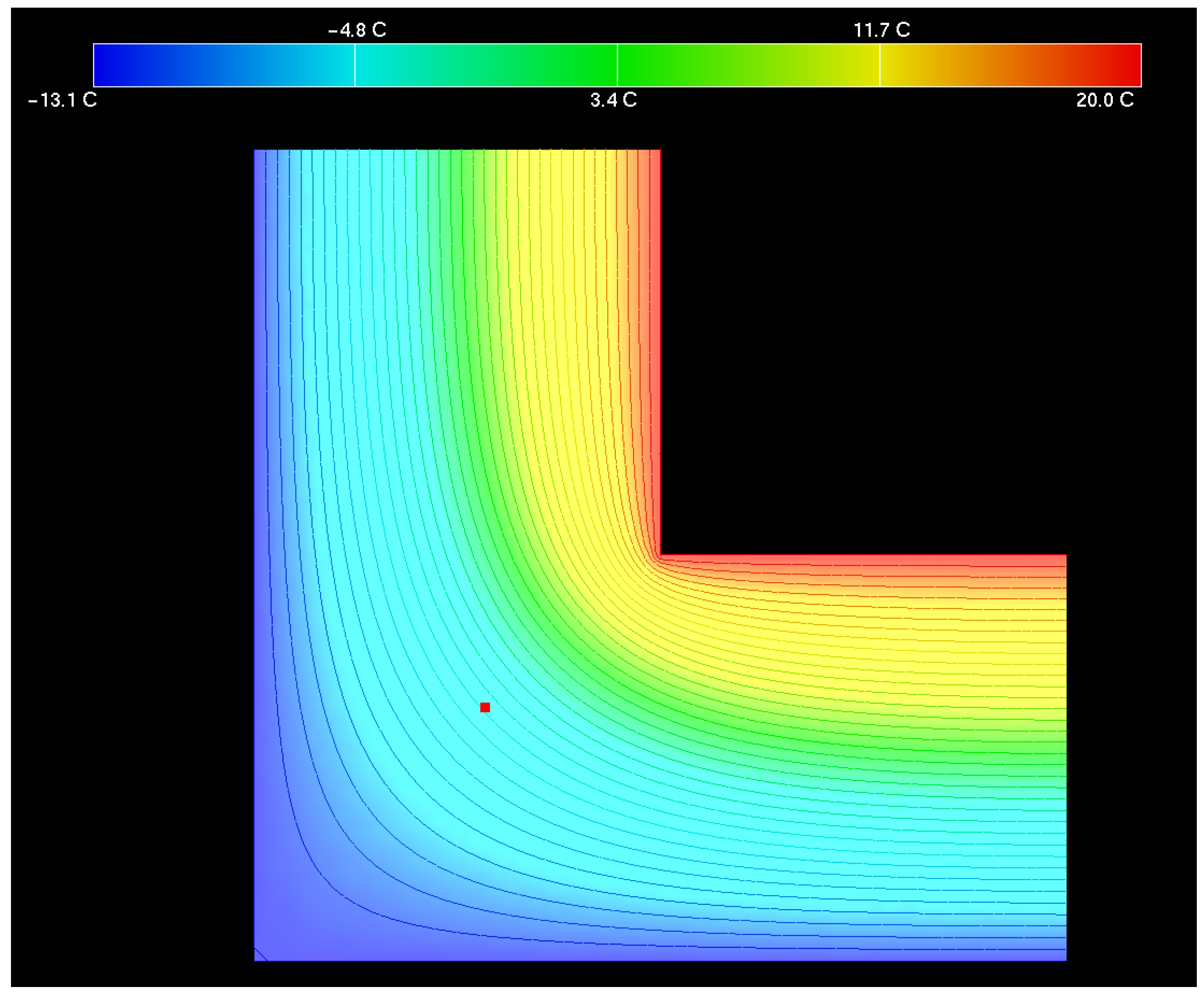
To illustrate a computational solution on a geometry that is somewhat similar but relevant in architecture, Figure 1 shows the solution of the heat equation on an interior edge. The effects of the boundary conditions are clearly visible: The hot and the cold boundary surfaces were given Dirichlet boundary conditions corresponding to 20 °C and −13.1 °C, respectively. The remaining two boundaries are given zero Neumann boundary conditions, resulting in the thermal isolines meeting those boundaries perpendicularly.
3.4.3. In Three Dimensions
Analogously to the preceding example, it is instructive to give the simplest case of a truly three-dimensional constant-time scalar field in a solid thermal bridge, such that it can not be simply reduced to the case of extrusion of a one- or two-dimensional scalar field along a perpendicular axis. Again, the value of an analytical solution is that it can be instructively obtained without reference to discretization, meshes and any numerical or computational aspects. It turns out that the simplest truly three-dimensional case of conductive heat transfer is that of an “igloo”—put simply, it is a semi-sphere between interior radius and exterior radius , kept at temperatures and . To find the simplest example, it suffices again to assume the same material everywhere, and the temperature field must obey Equation (4) where now is the three-dimensional Laplacian. Similarly to the preceding example, one finds that by the symmetry of the situation the temperature field can only depend on the distance r from the igloo’s center of symmetry, so that where . When using the expression for the Laplacian in spherical coordinates, it is easy to verify that the solution is where C and D are constants that depend only on but not on r or .
Along the ground level of the “igloo”, Neumann boundary conditions (see Section 4.1) are then obeyed as if the ground was a perfect insulator and also kept at temperatures and inside and outside, respectively, making this example not entirely unrealistic. Again, perhaps surprisingly, the temperature field does not depend on the material of the “igloo”. However, the total thermal dissipation, i.e., the required total thermal output of the igloo’s heating needed to keep the inside at temperature , does depend on the material’s conductivity and would be an easy and interesting exercise to calculate, using just the notions introduced in Section 2.
The relevance of this simplistic example is that the quantitative behavior of the heat flux—decaying with —is very different from the preceding example—where the decay is , highlighting the strong impact of passing from two to three dimensions. The same contrast can be observed when passing from an interior edge to an interior corner. This semi-analytical reasoning is even more important due to interior edges and corners being very fundamental geometries.
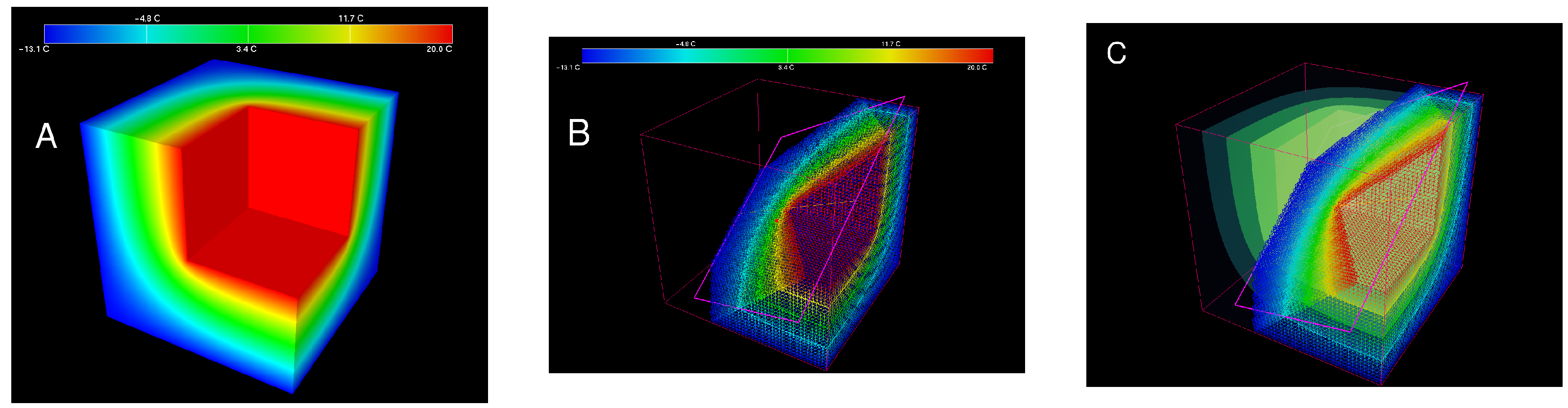
A similar and practically very relevant geometry is that of an interior corner. Figure 2 shows three views of the full three-dimensional temperature solution in a corner. Dirichlet boundary conditions were applied on the hottest (interior) and coldest (exterior) surfaces, and Neumann boundary conditions on all other surfaces. Note that the temperature isosurfaces meet the Neumann boundary surfaces perpendicularly. One can now compare the impact of passing from two to three dimensions: In Figure 1, the point , marked red, had temperature −6.5 °C, whereas in Figure 2B, the corresponding point—also marked red—only has temperature −10.7°C. This difference between 2D and 3D modeling highlights the necessity to treat thermal bridges volumetrically to achieve a realistic result. Under the assumption that the entire wall is of the same material the temperature does not depend on the material.
3.5. Existence and Uniqueness of Solutions
For completeness, one should indicate why Equation (2) does have any solutions at all—possibly with boundary conditions. To explain the steps of the proof one would require explaining not only the concept of weak solutions but also that of Sobolev spaces which would go beyond the scope of the entry. Suffice to say that the PDE Equation (2) is written as where D is the operator in the sense of functional analysis. One then verifies that this operator is strongly elliptic in the sense of Nirenberg [25] since its “symbol” is the expression and its “principal symbol”, its leading term is which is non-zero whenever is non-zero. Having a non-zero principal symbol whenever is what makes an operator “elliptic”; from there one can apply the existence and uniqueness theory of solutions to strongly elliptic differential operators as in (Evans [15], Chapter 6.2). This shows that there is a solution to our elliptic boundary value problem Equation (2) with Dirichlet boundary conditions on the interior and exterior surfaces and Neumann boundary conditions on the remaining surfaces. Moreover, this solution is unique.
4. Finite Elements—The Numerical and Computational Fundamentals
4.1. Boundary Conditions
4.1.1. Exterior and Interior Facing Surfaces—Dirichlet Boundary Conditions
When solving the temperature field, one applies the prior knowledge on exterior conditions. As mentioned earlier, one simplifies the simulation by erring on the conservative side and assuming that the surfaces that face the exterior and interior air masses are cooled and heated to the extreme temperatures −13.1 °C and 20 °C. The entire geometry of the thermal bridge shall be denoted by —the “problem domain”. Those surfaces of that are exposed to exterior or interior shall be denoted with S. The temperature u on S is known a priori. These kinds of boundary conditions are called Dirichlet boundary conditions in mathematical literature [15].
4.1.2. Structure Facing Surfaces—Neumann Boundary Conditions
The boundary of the domain shall be denoted by . Theses are all surfaces of of S but there are more surfaces that are part of , namely those that face the surrounding walls. Thus, the boundary of is a “Boolean union”—in the design and CAD sense—of S and its complement . The prior knowledge is that by definition a thermal bridge’s energy loss towards its surroundings in the structure are small compared to those from inside to outside. It therefore makes sense to have the integral lines of the heat flux to go from inside to outside but never into the neighboring or surrounding structure. This is equivalent to demanding that the isocurves of the temperature only go into surrounding structures since they are always orthogonal to the heat flux; see Figure 1. These kinds of boundary conditions are expressed by —the exterior normal derivative of u vanishes. This kind of boundary condition is called Neumann boundary condition.
4.2. Tetrahedral Meshes
The FE algorithm described above relies essentially on the existence of an accurate tetrahedral mesh decomposing the problem domain, i.e., the geometry of the thermal bridge. Accurate meshing of polyhedral domains into tetrahedra is an entire business on its own. A good starting point is the work of Shewchuk on constrained Delaunay triangulations; see Shewchuk and Brown [26], Hang [27], Geuzaine and Remacle [28] and the references therein. A good tetrahedral mesh of a given domain is:
- a collection of vertices—points in three-dimensional space, together with
- a collection of tetrahedra—quadruples of indices into the vertex list, together with
- a way of associating each tetrahedron with one and only one material.
Such that the following requirements are satisfied as best as possible:
- 1.
- The union of all tetrahedra covers the entire thermal bridge but no other volumes.
- 2.
- Each material corresponds uniquely to a subset of all tetrahedra.
- 3.
- The surfaces constituting the material boundaries are surface sub-meshes in the sense that faces that lie on the boundary are a surface mesh without topological defects. These surfaces appear as the “constraints” of the Delaunay triangulation.
- 4.
- Each tetrahedron should be “as equilateral as possible” in the sense that no interior edge angle among all vertices is less than a typical threshold of about .
4.3. Derivation of Algorithm for the Temperature Coefficients
This subsection will only introduce as many mathematical notions and notations as necessary for understanding just the particular case in question. The reader who is applying but not deriving the algorithm can gloss over the following details. While an introduction to FE methods can easily lead into deep waters of numerical and computational mathematics, it turns out that the case at hand allows for significant simplification with regards to the usual treatment in the literature. In numerical linear algebra, the simplest case of a problem is described by a collection of linear constraints. In this case, the columns of a matrix describing a linear problem correspond to the unknowns, and the rows correspond to the constraints. One can immediately translate this setup to the steady heat transfer problem, obtaining the following problem. Find the scalar field u on such that:
where is the exterior normal derivative—the derivative of the temperature in the outward facing direction at those parts of the boundary of that do not face exterior or interior air, for instance, the neighboring walls, or air pockets inside the wall. One needs Green’s first identity in the form
where is a vector field and is a scalar function. This variation of Green’s first identity is derived by applying the classical divergence theorem from vector calculus to the vector field and expanding the divergence with elementary rules. Applied to the heat flux , this identity yields:
Splitting this boundary integral over the two different boundary components , one further obtains:
where the function is not yet specified further—it holds for all such . After inserting our knowledge on the boundary conditions from Equation (5), one obtains
So far, this holds for all (reasonable) functions . One can now restrict the treatment to all functions where .
For all such functions that vanish on S, one indeed arrives at
Therefore, one has already arrived at what is commonly called the “weak” formulation of the problem Equation (5): Find u such that
Note that the boundary condition on the extreme temperatures at the interior and exterior facing walls needs to be imposed “externally”—it is called an essential boundary condition. In contrast, the Neumann boundary condition is taken care of automatically—which is known as a natural boundary condition. The role of is a test function—in analogy with the FE method in structural mechanics with the concept of “virtual displacement”, it could be called a “virtual temperature”. Let n be the number of vertices of the tetrahedral mesh. It makes sense to seek the values of the solution u at those vertices. Write for the unknown value of u at vertex i where . Once those values are found, the value of u at an arbitrary point will be approximated by simple linear interpolation.
where is a function on that is obtained by linearly interpolating a hypothetical solution that takes the value one at vertex i and the value zero at all other vertices. If the mesh was just a two-dimensional mesh, one could imagine plotting the “graph” of an analogously constructed function and that graph would look like a tent held up by a “pole” at vertex i, whence the choice of the letter t. In the mathematical literature, the functions would be called a “partition of unity” because everywhere on the mesh. To be explicit, the function can be constructed with the help of barycentric coordinates. Denote the barycentric coordinate of the point x inside a tetrahedron that is adjacent to vertex i with . Then
The numbers are the weights of the functions towards the solution u. In order to find an algorithm that approximates the numbers , one simply inserts Equation (12) into Equation (11). At the same time, it makes sense to only consider all of the tent functions that do not belong to vertices on S, as test functions. Henceforth, indices of vertices that are not on S will be denoted by j. Then, the weak formulation becomes: Find the coefficients on all vertices not on S such that
Note that those indeed vanish on S; hence, they satisfy the condition. Note that the sum over involves all vertices, including those corresponding to the vertices in S. The corresponding coefficients are non-zero. Therefore, Equation (14) is not just solved by the zero solution. To properly bring it into the form of a well-posed in-homogeneous linear problem, one applies the usual numerical procedure to “bring all known values to the right hand side”. Thus, one can subtract those summands, indexed by i, that correspond to vertices in S. Each index j determines a joint linear constraint on all the numbers . Conveniently, there are exactly as many constraints as unknowns, namely n minus the number of vertices in S. Now, it lends itself to abbreviate for a matrix A with n columns and n rows, one has arrived at the simple linear condition where, by a slight abuse of notion, the letter u refers to the vector . The matrix A is called the “stiffness” matrix, corresponding to the intuitive idea that if one of the coefficients is large and if for the sake of explanation the right hand side was not exactly zero but small and non-zero, then the corresponding term in the expansion was forced to be small; thus, a large stiffness permits only a small variation in the unknowns. One can assume that the vertices of the mesh are ordered in such a way that the ones in S come first. Then, the matrix A has a block structure: the upper left block of size , the lower right block of size , where are the numbers of vertices in S and in , respectively. From these formulas, one elementarily derives the following numerical solution scheme:
- Compute the lower right block of the stiffness matrix A as well as an appropriate sparse matrix factorization.
- Compute the lower left block —a rectangular sub-matrix with q rows and p columns.
- Assemble the vector of Dirichlet boundary components b; this is a vector of size p; solve the linear system of equations , resulting in the desired coefficients .
This completes the description of a basic FE scheme.
4.4. Extraction of Dissipation and U-Value from the Discretized Temperature
Given a temperature field u, it is easy to derive numerically all desired quantities. For instance, the discrete gradient operator [29] gives . Multiplication with interpolated on tetrahedra gives the thermal flux . Summation of all scalar products between outward facing normals at all interior surfaces with the thermal flux gives an approximation to which is the thermal dissipation. Division by gives the thermal conductance in W/K as defined in Section 2.4.6.
4.5. Norms and Standards
This subsection will gather the most important ISO norms pertinent to the physical quantities discussed above. It will focus on the ISO norms as these are the most widespread ones, with the largest international recognition.
The definitions of the physical quantities are given in ISO 7345:2018 [30]. ISO norm ISO 6946:2017 [31] treats the topic of surface resistance definitions in Section 2.4.5 above. There are two ISO norms just for particular thermal bridges: windows, doors and shutters: ISO 10077-1:2017 [32] and ISO 10077-2:2017 [33]. The definitions of assumed surface temperatures can be found in ISO 10211:2017 [21]. Calculation methods for non-stationary (dynamic) thermal properties are given in ISO 13786:2017 [34].
The industrial norm for measuring thermal conductivity as described in Section 2.4.2 is ISO 13787:2003 [35]. The minimal required interior surface temperatures necessary for vapor condensation and mold growth prevention is given in ISO 13788:2012 [36]. Finally, ISO 13789:2017 [37] describes methods used to determine effective thermal transmission coefficients for estimating convective heat transfer due to ventilation.
To give examples of the large differences between national regulations, the Canadian norm CSA Z5010 [38] describes the thermal bridging calculation methodology, whereas the German standard for thermal bridge insulation is DIN 4180-2 [18]. Further discussion of national and local norms and standards would go beyond the scope of this entry.
5. I-Beam
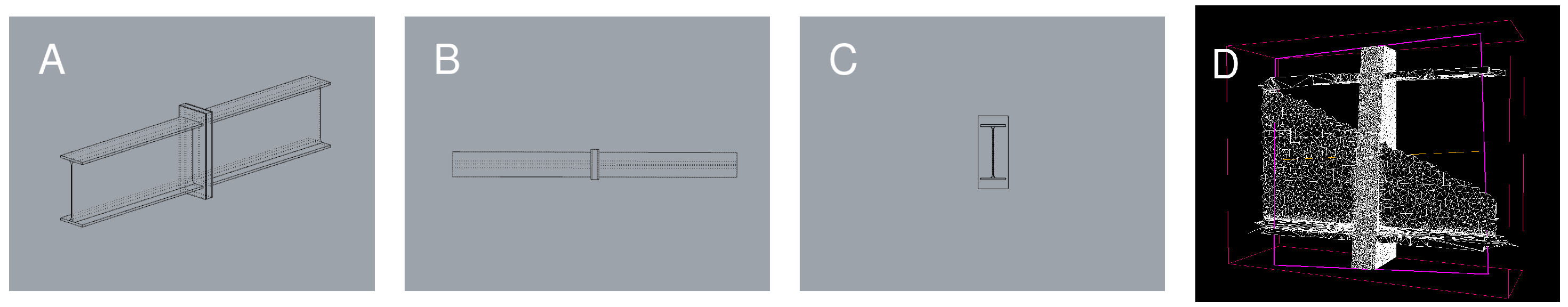
One of the most frequently occurring examples of thermal bridges are structurally required steel components that penetrate walls and are exposed both to exterior and interior air. Due to steel’s high conductivity, they are particularly prone to leaking heat. Figure 3 gives an overview of the geometry of an I-beam of type IPE400. A typical situation is where an I-beam penetrates a wall perpendicularly. The I-beam has an end on the outside—supporting a balcony, for instance, and the other end is on the inside, supporting a continuing wall slab. The ends are exposed to interior and exterior air masses at a distance of one meter each from the thermal break.
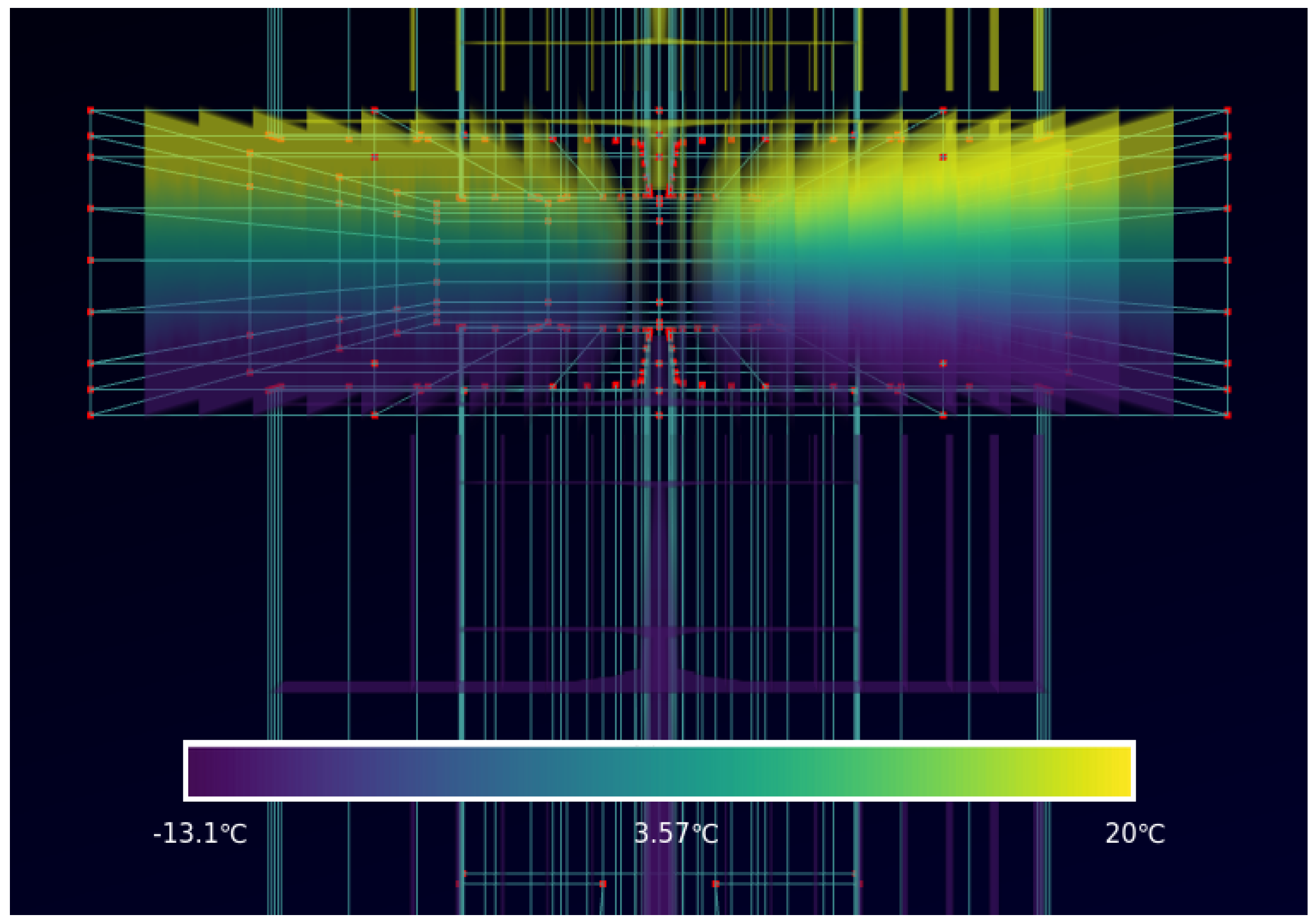
There are commercially available thermal breaks interrupting the I-beam orthogonally in such a way that the load bearing is guaranteed by screws joining two plates. For instance, a commercial solution is the popular “Schöck Isokorb” [39]. A typical question is whether this commercially available thermal break could be replaced with a potentially cheaper plastic insulator component without aggravating the vapor condensation risk. This thermal break consists of two large steel plates. The geometry was modeled in Rhino3D and meshed with the Gmsh meshing software [28], see Figure 3D. FE analysis, as described in the preceding section, reveals that this is not the case. The factor does not reach the critical threshold. The temperature at the interior facing side of the steel plate is only 11.9 °C. See Figure 4 for a visualization of the resulting temperature field. A 3D visualization is available at Fuchs [40].
6. Conclusions
In this entry, the paramount importance of accurate thermal modeling for energy-aware architecture has been pointed out. Filling this gap in the existing literature motivates this entry: Engineering texts often content themselves with approximations—that are often just one-dimensional such as the Glaser method or two-dimensional—without giving a full FE formulation. Texts on numerical methods describe the FE method in much more generality than is needed here, and mathematical literature on PDEs tend to describe only a variation of the equation that differs from the relevant one in two aspects: They often treat the time-dependent variant, and they consider a uniform material—this has the effect of abbreviating the divergence of the heat flux to a constant multiple of the Laplacian operator of the temperature. This obscures the equation’s physical meaning, and makes it pointless for engineering applications. In this entry, this gap has been filled, introducing the reader to the FE solution of the relevant steady state and isotropic but non-uniform heat equation. This entry first defined all relevant terms: Temperature gradient, heat flux, energy dissipation, U-values, thermal conductance. It then explained why the relevant equation is Equation (2) and that its physical meaning is that the heat flux does not “diverge”, in accordance with the absence of heating or cooling within the material, and that the intuitive notion of divergence actually corresponds to the divergence operator.
The notion of tetrahedral mesh was introduced, and how to obtain a computer-amenable discretization of the relevant steady state heat equation was also explained. This should have put the reader in a position to easily implement their own FE solver of the steady state heat equation, given a mesh that describes the given geometry in sufficient detail.
In a case study, a typical thermal bridge is an I-beam penetrating a wall. The question as to whether the insulation with plastic in the middle of the thermal break is sufficient was answered negatively—it turned out the interior facing surface temperature was not high enough to reliably prevent vapor condensation and mold growth.
The author hopes that the perusal of this entry has helped the reader gain an active understanding of the basic building blocks of the FE method for energy performance modeling, thereby putting them in a position to increase their maturity regarding sustainable architecture.
Funding
This research received no external funding.
Institutional Review Board Statement
Not applicable.
Informed Consent Statement
Not applicable.
Data Availability Statement
The software is available from the author. A software implementation of the core of the method—the solver—is contained in the materials to review.
Acknowledgments
English proofreading was done by Jamie Stangroom.
Conflicts of Interest
The author declares no conflict of interest.
Abbreviations
The following nomenclature, symbols and abbreviations are used in this manuscript:
| FEM | finite element method |
| PDE | Partial differential equation |
| thermal dissiplation | thermal energy loss per unit duration |
| Laplacian | the operator |
| scalar field | the assignment of a real number to each point |
| vector field | the assignment of a vector (three real numbers) to each point |
| time derivative of a scalar field | |
| ∇ | on a scalar field, its gradient; on a vector field, its divergence |
| gradient | the vector field given by the three partial derivatives of a scalar field |
| divergence | the scalar field given by the sum of the three |
| separate partial derivatives of a vector field | |
| stationary heat equation | the heat equation with ; synonym with steady state |
References
- Zienkiewicz, O.C.; Taylor, R.L.; Zhu, J.Z. The Finite Element Method: Its Basis and Fundamentals, 7th ed.; Elsevier/Butterworth Heinemann: Amsterdam, The Netherlands, 2013. [Google Scholar]
- Ciarlet, P.G. The Finite Element Method for Elliptic Problems; SIAM: Philadelphia, PA, USA, 2002. [Google Scholar]
- Wilson, E.L.; Nickell, R.E. Application of the finite element method to heat conduction analysis. Nucl. Eng. Des. 1966, 4, 276–286. [Google Scholar] [CrossRef]
- Lewis, R.W.; Morgan, K.; Thomas, H.; Seetharamu, K.N. The Finite Element Method in Heat Transfer Analysis; John Wiley & Sons: Hoboken, NJ, USA, 1996. [Google Scholar]
- Häupl, P.; Homann, M.; Kölzow, C.; Riese, O.; Maas, A.; Höfker, G.; Christian, N. Lehrbuch der Bauphysik: Schall-Wärme-Feuchte-Licht-Brand-Klima; Springer: Berlin/Heidelberg, Germany, 2017. [Google Scholar]
- Cody, B. Form Follows Energy: Using Natural Forces to Maximize Performance; Birkhäuser: Basel, Switzerland, 2017. [Google Scholar]
- Asdrubali, F.; Baldinelli, G.; Bianchi, F. A quantitative methodology to evaluate thermal bridges in buildings. Appl. Energy 2012, 97, 365–373. [Google Scholar] [CrossRef]
- Zalewski, L.; Lassue, S.; Rousse, D.; Boukhalfa, K. Experimental and numerical characterization of thermal bridges in prefabricated building walls. Energy Convers. Manag. 2010, 51, 2869–2877. [Google Scholar] [CrossRef]
- Arto, I.; Capellán-Pérez, I.; Lago, R.; Bueno, G.; Bermejo, R. The energy requirements of a developed world. Energy Sustain. Dev. 2016, 33, 1–13. [Google Scholar] [CrossRef]
- Kleinhückelkotten, S.; Neitzke, H.; Moser, S. Repräsentative Erhebung von Pro-Kopf-Verbräuchen natürlicher Ressourcen in Deutschland (nach Bevölkerungsgruppen); Umweltbundesamt: Dessau-Roßlau, Germany, 2016. [Google Scholar]
- Khazal, A.; Sønstebø, O.J. Valuation of energy performance certificates in the rental market—Professionals vs. nonprofessionals. Energy Policy 2020, 147, 111830. [Google Scholar] [CrossRef]
- Terms and Conditions; Ansys Fluent; Ansys: Canonsburg, PA, USA, 2015; Available online: https://www.ansys.com/academic/terms-and-conditions (accessed on 1 April 2022).
- Hecht, F. New development in FreeFem++. J. Numer. Math. 2012, 20, 251–265. [Google Scholar] [CrossRef]
- Déqué, F.; Ollivier, F.; Roux, J. Effect of 2D modelling of thermal bridges on the energy performance of buildings: Numerical application on the Matisse apartment. Energy Build. 2001, 33, 583–587. [Google Scholar] [CrossRef]
- Evans, L.C. Partial Differential Equations; American Mathematical Society: Providence, RI, USA, 2010. [Google Scholar]
- Sawhney, R.; Crane, K. Monte Carlo Geometry Processing: A Grid-Free Approach to PDE-Based Methods on Volumetric Domains. ACM Trans. Graph. 2020, 39, 123. [Google Scholar] [CrossRef]
- Grossmann, C.; Roos, H.G.; Stynes, M. Numerical Treatment of Partial Differential Equations; Springer: Berlin/Heidelberg, Germany, 2007; Volume 154. [Google Scholar]
- Din Norm. DIN Norm 4180-2: Thermal Protection and Energy Economy in Buildings—Part 2: Minimum Requirements to Thermal Insulation; Din Norm: Berlin, Germany, 2012. [Google Scholar]
- Taylor, B.J.; Cawthorne, D.; Imbabi, M.S. Analytical investigation of the steady-state behaviour of dynamic and diffusive building envelopes. Build. Environ. 1996, 31, 519–525. [Google Scholar] [CrossRef]
- Gasparin, S.; Berger, J.; Dutykh, D.; Mendes, N. Solving nonlinear diffusive problems in buildings by means of a Spectral reduced-order model. J. Build. Perform. Simul. 2019, 12, 17–36. [Google Scholar] [CrossRef]
- ISO. Norm 10211: Thermal Bridges in Building Construction–Heat Flows and Surface Temperatures–Detailed Calculations; ISO Norm, Vernier: Geneva, Switzerland, 2017. [Google Scholar]
- Gerthsen, C.; Vogel, H. Physik, 17. Auflage; Springer: Berlin/Heidelberg, Germany, 1993. [Google Scholar]
- Walter, W. Gewöhnliche Differentialgleichungen. Eine Einführung; Springer: Berlin/Heidelberg, Germany, 2000. [Google Scholar]
- Glaser, H. Vereinfachte Berechnung der Dampfdiffusion durch geschichtete Wände bei Ausscheidung von Wasser und Eis. Kältetechnik 1958, 10, 358–364. [Google Scholar]
- Nirenberg, L. Remarks on strongly elliptic partial differential equations. Commun. Pure Appl. Math. 1955, 8, 649–675. [Google Scholar] [CrossRef]
- Shewchuk, J.R.; Brown, B.C. Fast segment insertion and incremental construction of constrained Delaunay triangulations. Comput. Geom. 2015, 48, 554–574. [Google Scholar] [CrossRef]
- Hang, S. TetGen, a Delaunay-based quality tetrahedral mesh generator. ACM Trans. Math. Softw. 2015, 41, 11. [Google Scholar]
- Geuzaine, C.; Remacle, J.F. Gmsh: A 3-D Finite Element Mesh Generator with built-in Pre- and Post-Processing Facilities. Int. J. Numer. Methods Eng. 2009, 79, 1309–1331. [Google Scholar] [CrossRef]
- Mancinelli, C.; Livesu, M.; Puppo, E. A comparison of methods for gradient field estimation on simplicial meshes. Comput. Graph. 2019, 80, 37–50. [Google Scholar] [CrossRef]
- ISO. Norm 7345: Thermal Performance of Buildings and Building Components—Physical Quantities and Definitions; ISO Norm, Vernier: Geneva, Switzerland, 2018. [Google Scholar]
- ISO. Norm 6946: Building Components and Building Elements—Thermal Resistance and Thermal Transmittance—Calculation Methods; ISO Norm, Vernier: Geneva, Switzerland, 2017. [Google Scholar]
- ISO. Norm 10077-1: Thermal Performance of Windows, Doors and Shutters—Calculation of Thermal Transmittance—Part 1: General; ISO Norm, Vernier: Geneva, Switzerland, 2017. [Google Scholar]
- ISO. Norm 10077-2: Thermal Performance of Windows, Doors and Shutters—Calculation of Thermal Transmittance—Part 2: Numerical Method for Frames; ISO Norm, Vernier: Geneva, Switzerland, 2017. [Google Scholar]
- ISO. Norm 13786:Thermal Performance of Building Components—Dynamic Thermal Characteristics—Calculation Methods; ISO Norm, Vernier: Geneva, Switzerland, 2017. [Google Scholar]
- ISO. Norm 13787: Thermal Insulation Products for Building Equipment and Industrial Installations—Determination of Declared Thermal Conductivity; ISO Norm, Vernier: Geneva, Switzerland, 2003. [Google Scholar]
- ISO. Norm 13788: Hygrothermal Performance of Building Components and Building Elements—Internal Surface Temperature to Avoid Critical Surface Humidity and Interstitial Condensation—Calculation Methods; ISO Norm, Vernier: Geneva, Switzerland, 2012. [Google Scholar]
- ISO. Norm 13789: Thermal Performance of Buildings — Transmission and Ventilation Heat Transfer Coefficients — Calculation Method; ISO Norm, Vernier: Geneva, Switzerland, 2017. [Google Scholar]
- ISO. Norm CSA Z5010: Thermal Bridging Calculation Methodology; ISO Norm: Toronto, ON, Canada, 2021. [Google Scholar]
- Müller, M.; Li, Z.; Standeker, J. Schöck Isokorb®–Gebrauchstauglichkeit unter Berücksichtigung der Langzeiteigenschaften. Beton-Und Stahlbetonbau 2020, 115, 35–43. [Google Scholar] [CrossRef]
- Fuchs, M. I Beam Thermal Break Visualization. Available online: https://mathiasfuchs.com/rawtetgen.html (accessed on 31 March 2022).
Figure 1.
A two-dimensional solution on an interior edge, the point marked with a red cross.

Figure 2.
(A) A three-dimensional solution on an interior corner. (B) A section of the solution containing the point , marked with a red cross. (C) A generic section.
Figure 2.
(A) A three-dimensional solution on an interior corner. (B) A section of the solution containing the point , marked with a red cross. (C) A generic section.

Figure 3.
(A) The I-beam IPE400 with a thermal break in parallel perspective projection. (B) Top view. (C) Right view. (D) Section of the tetrahedral mesh.
Figure 3.
(A) The I-beam IPE400 with a thermal break in parallel perspective projection. (B) Top view. (C) Right view. (D) Section of the tetrahedral mesh.

Figure 4.
The solution of the I-beam temperature field.

Publisher’s Note: MDPI stays neutral with regard to jurisdictional claims in published maps and institutional affiliations. |
© 2022 by the author. Licensee MDPI, Basel, Switzerland. This article is an open access article distributed under the terms and conditions of the Creative Commons Attribution (CC BY) license (https://creativecommons.org/licenses/by/4.0/).
Share and Cite
MDPI and ACS Style
Fuchs, M. Conductive Heat Transfer in Thermal Bridges. Encyclopedia 2022, 2, 1019-1035. https://0-doi-org.brum.beds.ac.uk/10.3390/encyclopedia2020067
AMA Style
Fuchs M. Conductive Heat Transfer in Thermal Bridges. Encyclopedia. 2022; 2(2):1019-1035. https://0-doi-org.brum.beds.ac.uk/10.3390/encyclopedia2020067
Chicago/Turabian StyleFuchs, Mathias. 2022. "Conductive Heat Transfer in Thermal Bridges" Encyclopedia 2, no. 2: 1019-1035. https://0-doi-org.brum.beds.ac.uk/10.3390/encyclopedia2020067