
QoE Modeling on Split Features with Distributed Deep Learning


1
Ericsson AB, 164 83 Stockholm, Sweden
2
Department of Technology and Aesthetics (DITE), Blekinge Institute of Technology, 374 24 Karlshamn, Sweden
*
Authors to whom correspondence should be addressed.
Network 2021, 1(2), 165-190; https://0-doi-org.brum.beds.ac.uk/10.3390/network1020011
Submission received: 6 July 2021
/
Revised: 20 August 2021
/
Accepted: 26 August 2021
/
Published: 28 August 2021
Abstract
:The development of Quality of Experience (QoE) models using Machine Learning (ML) is challenging, since it can be difficult to share datasets between research entities to protect the intellectual property of the ML model and the confidentiality of user studies in compliance with data protection regulations such as General Data Protection Regulation (GDPR). This makes distributed machine learning techniques that do not necessitate sharing of data or attribute names appealing. One suitable use case in the scope of QoE can be the task of mapping QoE indicators for the perception of quality such as Mean Opinion Scores (MOS), in a distributed manner. In this article, we present Distributed Ensemble Learning (DEL), and Vertical Federated Learning (vFL) to address this context. Both approaches can be applied to datasets that have different feature sets, i.e., split features. The DEL approach is ML model-agnostic and achieves up to accuracy improvement of ensembling various generic and specific models. The vFL approach is based on neural networks and achieves on-par accuracy with a conventional Fully Centralized machine learning model, while exhibiting statistically significant performance that is superior to that of the Isolated local models with an average accuracy improvement of . Moreover, energy-efficient vFL with reduced network footprint and training time is obtained by further tuning the model hyper-parameters.
1. Introduction
Quality of Experience (QoE) addresses the degree of user delight or annoyance [1]. For service and network providers, it is important to control the factors that contribute to QoE, which are captured by QoE models. The ultimate goal for QoE modeling is to develop a QoE model that accurately predicts QoE under any circumstances and in any contexts. However, due to different contexts and facilities, such local datasets can be very different from each other in scope and contents, which makes it hard for a generic model to capture the local conditions and adapt the QoE predictions accordingly.
QoE modeling is challenging due to QoE assessment being multi-dimensional, user-centric, multi-sensory [2], and decentralized by its nature due to a high number of naturally distributed QoE indicators and contributing factors. Accordingly, observations of different users, application, and network aspects need to be performed and coordinated. These requirements are hard to meet, due to the efforts and costs of subjective user studies and various QoE assessment tools. To achieve a superior QoE model, a comprehensive user study that covers all possible contexts is required, where the collected datasets are eventually shared publicly to advance reproducible research. While ML is promising due to its capability of mining large amounts of data that consists of high number of confounding factors, it also brings about a set of challenges, foremost data privacy aspects and specific machine learning issues revolving around the diversity that different datasets may have in terms of their different feature space.
From generation to generation, every network technology is expected to outperform its predecessor in terms of capacity, coverage and QoE, accompanied by increased demands for sustainability [3]. Furthermore, networks are expected to become increasingly dense [4], thus requiring greater adoption of the edge computing paradigm to reduce latency and protect data privacy. Consequently, end-to-end data collection, network performance monitoring and development of forecasting models for network performance prediction and/or QoE estimation, will be even harder due to the inherently distributed observations at different parts of the network path such as RAN (Radio Access Network), transport, and applications, which are expected to be provisioned by different business segments such as operators and service providers. Eventually, all measurements performed on different segments need to be shared to compute overall end-to-end QoE. This necessitates efficient and automated enablers such as distributed machine learning on multiple non-shared datasets that have potentially different feature sets. This way, a complete QoE model can be assembled leveraging end-to-end distributed single observations from different applications, networks, and energy performance sensors.
1.1. QoE Machine Learning Challenges
Towards achieving a superior QoE model, a comprehensive user study that covers all possible contexts is required in principle, where the collected datasets are eventually shared publicly to advance reproducible research. Machine learning models might be appealing especially when the corresponding feature set is large and complex with very large datasets [5]. On the other hand, there are data privacy aspects that need to be preserved, hence data may not be copied/transferred, processed, or modeled in a centralized computation node in a Fully Centralized way. Even so, continuous shuffling and transfers of large size sets of raw data is costly and energy-consuming. The overall ML challenges related to QoE modeling are itemized as follows:
- Model transfer might be inadequate: QoE data in the source domain (the domain that trains and sends out the pre-trained model), where the model is developed, and QoE data in the target domain (the domain that receives and uses the pre-trained model received from the source domain), where the model is to be deployed for real operations, need to have a similar data distribution as they need to represent the same underlying conditions and features. The authors of [6] show that when a model is trained with features that are only specific to the source domain, negative transfer (reducing the model performance) can occur, since the specific features at the source domain do not represent the target domain well enough. In addition, model transfer might leak information from the source domain to the target domain since there is no intermediate aggregation process before the target domain receives the model.
- Privacy-sensitive dataset: Specific local features in the source domain are potentially sensitive; detailed user profiles, among others, cannot be shared easily [7] without explicit consent. In addition, it may happen that one research group is interested in a QoE model particularly for video contents with high spatio-temporal complexity, e.g., within the scope of developing action games, while another research group is interested in assessing QoE for a different type of video content. At the same time, there might still be a common subset of non-sensitive indicative metrics, i.e., ML features, representing the underlying QoE factors in multiple domains or decentralized entities.
- Distributed user observations with different features: Model training can be inherently split into multiple partitions in cases when datasets are collected at multiple physically separated computation nodes. A typical example is when operators collect network datasets, while applications collect User Equipment (UE)-specific datasets on the application layers and user interfaces of applications. Another example is that some QoE research entity collects a user dataset with observations that are different from those obtained by other research entities. For example, operators that serve different customer segments, with different preferences and expectations might have different user profiles. These two datasets can be trained on separate models, which are trained only on local features, but collaboratively to improve local model accuracies further with minimally exchanged information in between.
1.2. Distributed Learning in QoE
As of today, two non-distributed learning techniques are most common in QoE modeling, (e.g., in crowd-sourcing based QoE assessment techniques, QoE databases that require special access): Isolated and Fully Centralized, and we use the two as reference scenarios. The most conventional technique for QoE model training today is Isolated, where every entity trains individual decoupled machine learning models on the locally collected inherently decentralized datasets. We also use a Fully Centralized learning technique as a reference as this is an existing way of QoE model training in the community in the cases when moving data in between entities is not an issue. In a Fully Centralized reference scenario, all training datasets are collected into one physical storage where the training of all dataset is performed. Opposed to this, a local dataset is visible only to its owner (where the data originates from) and the single computation node that collects the dataset trains the model. The comparison between conventional Fully Centralized and Isolated machine learning model training methodologies in the scope of QoE is given in Figure 1.
Distributed learning techniques can be split into two major categories: model-parallel and data-parallel based on the state-of-the-art distributed learning survey [8]. Accordingly, we position our article as stated in bold in Figure 2. In the model-parallel category, datasets can be shared from where they are originally produced/collected, and multiple models with the exact same type and architecture are used in the training. The main goal is to utilize more resources in parallel for faster computation and training. In this scenario, the datasets are completely or partially accessible by other computation nodes, by means of redistributing and reshuffling of datasets among those nodes. All collaborating nodes can communicate and share parameters and some data with each other. In the data-parallel category, both models and datasets are not necessarily identical, and datasets cannot be shared from where they are originally produced and collected. The main goal here is to reduce the privacy leakage of a raw dataset by avoiding moving raw data, making this solution an enabler for combining the individual learned knowledge from individual local models and from inherently decentralized datasets. In this scenario, the individual workers can share only trained model parameters in between each other in a fully- or semi-decentralized way, as in the case of gossip learning [9]. In case any direct communication in between workers is not allowed, two main groups can be presented: (i) Horizontal Federated Learning (hFL), in which the models need to train on the exact same feature set. (ii) Distributed Ensemble Learning (DEL) and Vertical Federated Learning (vFL), in which feature sets are not necessarily identical. Existing hFL techniques [10,11] enable model training without moving datasets in between different computation nodes by means of sending an aggregation of model parameters. Yet, hFL necessitates all computation nodes to have the same observation attributes or, more specifically, ML feature sets. In the cases where the feature sets are different in between collaborating computation nodes of research entities due to a distributed heterogeneous sensor environment, other decentralized learning techniques that permit collaborative training with distributed unique attributes in each computation node are necessary to be considered.
Therefore, in this article, we mainly study two distributed data-parallel-based learning techniques for datasets that are potentially and inherently decentralized in feature space: (i) a baseline DEL technique; (ii) a Distributed Split Learning (SplitNN)-based vFL technique [12,13] with partial neural networks. A combination of predictions of different independent trained models, is known to perform better than each model alone [14]. DEL is a technique that utilizes that property by averaging the output of the pre-trained models at the source domain(s) with the target domain model output to maximize the accuracy at the target domain. The datasets in the source domains need to have at least a subset of the feature set of the target domain. It is a suitable technical solution, but requires tuning the weights between the source, and the target model by monitoring metrics that quantify data diversity such as Kullback–Leibler (KL) divergence [15]. We mainly propose and evaluate vFL, which is based on a split neural network architecture, where each split partition of one big neural network (NN) model can reside on different physical computation nodes. This allows each worker to train a NN model jointly even on completely different feature sets on each participating node. In addition, since all worker nodes including the master node collaborate to train one single machine learning model, the information exchange in between them is bidirectional. The requirement is a consensus and synchronization in between the participating nodes about the task they are solving. In the case of multi-sensor distributed local datasets, e.g., IoT datasets, the observations that are collected on different distributed local nodes need to be from the same time interval. Similarly, in the case of QoE user studies, any observations that are collected via different measurement modules from the same users in different labs would need to follow the same sequential way of assessment. It could be for instance also applicable in the cases of a very large-scale user study where many participants experience the exact same video (or accomplish the same task), while every research entity considers only subparts of the observations of the subjects due to limitations of sensor availability, or assessment tools in the user labs. For instance, one research entity is collecting data from one particular user with sensor set A, while another entity uses sensor set B.
The main differences between DEL and vFL techniques are illustrated in Figure 3. The local feature sets are denoted by S0 and S1 for the groups 0 and 1, respectively. The trained models in every node are denoted by , where i denotes the group id where M is trained. The target variables that the models aim to estimate are denoted by . In DEL, the pre-trained model at the source domain (G1) with features S1 is transferred to the target domain (G0). Two separate inference processes are then executed at G0; one via the received model with generic features S1, and one with model with both S0 and S1. Finally, the two outputs from the two models, are averaged to obtain the final model output. In vFL, there is no transfer of model from source to target domain, instead they are trained jointly. The intermediate representation output at the cut-layer of the neural network models in vFL in both groups are given with matrices, . The latter are then transferred to the master node and are used as input to the master neural network model. Finally, the joint model output is obtained. In DEL and vFL, there is no requirement for the computation nodes to have the exact same set of attributes. In DEL, the source domain should have at least a subset of the features of the target domain (e.g., shareable non-sensitive feature subset); and in vFL, the attributes can be totally orthogonal as they can be completely decoupled. Detailed descriptions of DEL and vFL are given in Section 5. Overall, we consider vFL to be more flexible than DEL and consider DEL as rather a baseline.
Our contributions differentiate from prior-art as follows:
- Low-level NumPy based framework for split-learning: Our vFL implementation is based on Split Neural Network (SplitNN) [12], but unlike PySyft [16], it does not operate on existing frameworks with high level abstraction such as TensorFlow or PyTorch. Hence, the most important difference in our framework is that we have full control including the communication protocol and the algorithms. This enables low level algorithmic development to optimize for computation, privacy, network footprint, training time, and energy-efficiency while sustaining good and robust model development in diverse scenarios especially in heterogeneous data settings. Our framework is not limited to a simulation on a single node and can easily be deployed on a Kubernetes cluster.
- A comparison of different techniques for training datasets with different feature spaces: In this article, we present Distributed Ensemble Learning (DEL), and Vertical Federated Learning (vFL) to address the aforementioned challenge. These techniques are appealing for different domains including the telecommunication segment where datasets are typically decentralized. The DEL approach is machine learning model-agnostic, while the vFL approach is based on neural networks. Furthermore, we recommend a few techniques to reduce network footprint, training time, and energy consumption of the model training process.
- Jointly trainable QoE modeling with split features: While we are demonstrating our vFL solution in this article, to the best of our knowledge, this work is the first of its kind, that demonstrates a QoE model training in a distributed deep learning setting with split features.
This article is structured as follows: In Section 2, we first present related work on hFL, DEL, and vFL. Section 3 presents the dataset and the feature description, that is then followed by a motivation of a QoE use case related to attribute splitting in Section 4. The contribution of each attribute to the model prediction is studied in detail, and compared via a use case where content-based features such as Temporal Complexity index (TI) and Spatial Complexity index (SI) cannot be shared. Section 5 presents the vFL technique together with a baseline DEL technique. Results including the model performance evaluation and comparison of different experiment scenarios from the two approaches are given in Section 6. The article is concluded in Section 7 along with a brief discussion on limitations and directions for future work.
2. Related Work
Decentralized and distributed learning techniques such as ensemble learning, transfer learning, and federated learning are well-known [17], and we foresee the importance of these methods in future generation mobile network architectures, especially since we see these techniques as enablers for energy-efficient QoE modeling while preserving privacy. Yet, there exists very little work in the literature that leverage decentralized learning technologies such as federated learning in QoE [11].
- Horizontal Federated Learning (hFL): In horizontal federated learning [10], models are trained collaboratively by combining different models which have been trained locally on the same feature set, to a single model at a master node. When such a model is shared back to the individuals that contributed to the training process, immediate benefits can be detected for those that have similar data distribution representing similar underlying conditions and context. In [18], feature selection is studied within Neural Network-based Federated Learning, where model parameters are divided into private and federated parameters. Only the federated parameters are shared and aggregated during federated learning. It is shown that this model customization approach significantly improves the model performance while not sharing raw data in between.
- Distributed Ensemble Learning (DEL): In [19], the authors used transfer learning to estimate the labels of an unlabeled dataset where the labels represent user emotions. In [11], a Round Robin-based learning technique (inspired by Baidu-AllReduce [20]) is presented within the scope of web QoE. This approach, similar to hFL, requires the distributed domains to have at least a subset of the features (if not all) to be the same.
- Vertical Federated Learning (vFL): Vertical federated learning enables collaborating nodes to jointly train a machine learning model with fully orthogonal feature sets. Most relevant vFL implementations in the literature are: PaddleFL [21], PySyft [16], FATE [22], and FedML [23]. Although all of the above solutions indicate great progress, PaddleFL, FATE, and PySyft implementations were inadequate for our needs due to their high level abstraction. The closest implementation among them all is FedML; however, we have not yet performed a complete comparison with that work and ours as it was very recently published.
- Privacy-preserving communication: It is shown in the literature [24] that sending model weights that emerged from training, instead of sending the actual raw dataset, may still leak sensitive information about the ground truth used to train the model. Therefore, there exist techniques to further protect privacy on the shared weights of the models. Techniques such as differential privacy [25] and secure aggregation [26] can be utilized for sharing private information for the purposes of training ML models without revealing the original dataset and also concealing the identity of the dataset’s origin. In DEL, only the generic model (architecture and internal representation) is shared, which is already known and as such does not need to be protected. In the scope of this study, we consider these techniques as complementary since they can be applied to hFL or vFL without affecting the inner workings of each approach.
- QoE modeling with ML: ML techniques have been studied previously in QoE modeling [29]. Furthermore, a mix of conventional and a ML based QoE modeling has been implemented and demonstrated previously in [30]. All existing QoE models are trained via Fully Centralized manner. Our proposed vFL in this article, can be considered as a good candidate solution to ensemble local models at the workers without predefined model weight thresholds, and without necessitating the NN models to be of the same architecture and feature space.
To address the intersection of challenges given in Section 1.1 and Section 1.2, it is important to develop energy-efficient, privacy-preserving, and scalable ML model training solutions that satisfy decentralized requirements, and we think that it is only possible via tools that help innovate via low level algorithmic development such as in the vFL framework that we demonstrate in this article.
3. Dataset and Feature Extraction
The publicly available QoE dataset Waterloo Streaming QoE Database III (SQoE-III) [31] is used in this article. It has been collected using a well-grounded user study methodology. The MOS scores on the dataset are highly correlated (higher than ) with well-known QoE models such as P.NATS [32]. The dataset consists of 20 raw HD reference DASH videos, where the video length is 13 s on average. The experiments are performed while changing the video streaming bandwidth amongst 13 different bitrate levels ranging from Mbps to Mbps. The switch is performed in six categories; stable, ramp-up, ramp-down, step-up, step-down, and fluctuation. The video sequences vary in spatio-temporal complexity. TI (Temporal Information) is a measure of how the consecutive frames differ from each other in time, while SI (Spatial Information) is a measure of how the pixels in a given frame differ in between each other [33]. In the dataset, SI values are between 35 and 160; while TI values are between 11 and 114. There were 34 subjects (ages range between 18 and 35) involved in the study. Four of which provided outlier ratings that had to be removed. The user ratings are collected using a rating scale, where the scores are between 0 (worst) and 100 (best). The number of samples in the dataset was 450.
We extracted the 9 features as described in Table 1 from the raw dataset. The feature names are also depicted with a split index such that the features that are less than the applied split index are placed in feature subset S0, while the remaining features are placed in feature subset S1, respectively. For example, if the split index is set to 4, the features TI, SI, FPS and lastBitrate are placed in feature subset S0; and the remaining features nstalls, stallTimeInitialTotal, stallTimeIntermediateTotal, bitrateTrend, and meanBitrate (as far as it exists in the scenario) are placed in feature subset S1. In DEL, the group 0 (target domain) has feature set S0, and the group 1 (source domain) has feature set S1. In vFL, S0 features are in group 0 (worker 0), and S1 features are in group 1 (worker 1).
4. Effect of Video Content on QoE
In this section, in order to motivate the use of split learning in QoE, we quantify the effect of individual features on the QoE estimation, in particular the MOS label. We consider an example QoE use case with splitting of the features according to different split indexes. We test and experiment with different feature split assumptions. In the dataset, we hypothesize through domain expertise that the specific features are the ones related to the spatio-temporal content complexity, represented by the TI and SI features. In order to quantify the effect of the video content, in particular, on the QoE modeling, we performed at least 100 experiments to achieve statistical significant comparison of scenarios. In each experiment, we randomly select of data as training set, and as test set. We use the coefficient of determination and mean absolute error (MAE), indicating the mean absolute difference between the true label and the predictions, as accuracy evaluation metrics. confidence interval half-sizes are also obtained. XGBoost model of a Python Scikit-learn [34] implementation was used and the hyper-parameters were set as follows: eta to , maximum depth to 4, subsample to , subsample ratio of columns when constructing each tree to 1, and objective function’s evaluation metric to root mean squared error.
4.1. Training with or without Content Features
We first train an XGBoost [34] (a robust widely used tree-based ensemble ML algorithm) both with and without the specific TI and SI features. Next, the model accuracy performance of each case is compared. We observe that the inclusion of content-related features, i.e., TI and SI, makes the model a more powerful predictor with a rather high score (an increase from ± 0.01 to ± ) and low MAE (a decrease from ± to ± ), indicating that content-related features are important QoE factors.
4.2. SHAP Sensitivity Analysis
We use the TreeExplainer by SHAP [35] to apply sensitivity analysis and observe the features that are important for the decision of the trained ML model. In Figure 4, the effect of each input feature on model prediction is quantified from most to least important (descending order from top to bottom on the y-axis). Red regions indicate that the absolute value of the effect of the feature on the model prediction is high, while blue regions indicate the contrary. The dots being on the positive side of the x-axis indicate that the effect is positive, a higher feature value contribute to a higher MOS, and vice-versa if they are located on the negative side. The SHAP diagram indicates that the average bitrate (meanBitrate) is the most important metric in the model prediction, contributing to raising the MOS value as expected. Similarly, the total video stall duration, stallTimeIntermediateTotal, has a high influence on the negative side, which implies that it tends to lower the expected MOS value. The TI and SI features are considered more important than other features such as the number of stalls, nStalls, and the initial stalling time, stallTimeInitialTotal.
5. Distributed Learning Approaches on Split Feature Scenarios
We study two distributed learning techniques as detailed in this Section, DEL and vFL. In this experiment setup, we formulate both problems as binary classifications. The labels that are ranging between 11 and 97 are quantized into two classes: the values that are less than the median of the MOS scores (62) are considered to be the “poor-or-worse” class 0, and the labels that are more than the median of the MOS scores are considered to be the “good-or-better” class 1. Different from the state-of-the-art [36] definition of this split, we do not put a buffer zone between the two classes as was done for instance in the E-model, in order not to decrease the sample size in the dataset further.
In the experiments under this Section, the performance evaluation of the corresponding scenarios are performed via at least 10 iterations. Due to the binary classification formulation of the estimation models, evaluation metrics such as precision, recall, and F1-score are considered. Precision is a measure that calculates the ratio between the number of true “good-or-better” estimations and the total number of “good-or-better” estimations, i.e., the number of true positives divided by the sum of numbers of true and false positives. Recall is the ratio of true “good-or-better” estimations to the number of actual “good-or-better” values, i.e., the number of true positives divided by the sum of the number of true positives and the number of false negatives. The harmonic mean of precision and recall yields the F1-score in decimal points ranging between 0 and 1. A higher F1-score indicates a better-performing model.
We use boxplots, confidence intervals and the Dunn post hoc test [37] to quantify the pair-wise statistical significant difference between the scenarios. We evaluate the F1-score model accuracy on the test sets, after the training phase is completed. The improvement percentages of accuracy values, x, are computed as given in Equation (1).
For example, if the mean F1-score of all experiment iterations of scenario A is ; and if the mean F1-score of all experiment iterations of scenario B is ; and if the two distributions are statistically significantly different according to Dunn post hoc test (p-value less than 0.05), then we consider a statistical significant improvement in F1-score in Scenario B as opposed to Scenario A.
5.1. Neural Network
The Neural Network algorithm [38], is used in this study, which consists of matrix-like located neurons that are connected to each other over multiple layers. The higher the number of layers, the deeper a neural network becomes. The neurons on the same layer are not connected within each other but only to the neurons in the previous and/or in the next layer. In a forward pass, a linear transformation at every neuron occurs, where the outputs from the previous layer are computed via a weighted sum followed by addition of some bias. Next the outputs of each neuron undergo a non-linear transformation via the activation function and then passed to all or a subset of neurons of the next layer of the neural network. The error computation is made at the layer where the ground-truth actual labels are present. Depending on the magnitude of the computed error, the weights of every neuron are re-adjusted with a gradient operation (partial derivative), in other words aiming at minimizing the final computed loss. This is called backwards propagation. One can also adjust when to update the neuron weights by setting the hyper-parameter called batch size. If the batch size is set to B, then the model weights will be updated at every time all neurons process B samples amongst the whole set. This is repeated sequentially for multiple rounds on all layers, first via forwards propagation from left-to-right, and then later via backwards propagation right-to-left, until the error does not decrease anymore. At this point, the model is considered as converged. The higher the B, the more time it takes the model to update its weights, while very small B makes the model weights update very frequently. Therefore, a suitable B needs to be selected. Epoch is the number of times the whole neural network sees all training samples. In the case of N training samples, and if all batches are different and complementary, it then mathematically takes rounds (i.e., all sample set size divided by the batch sample set size) for the model to perform one epoch of training. We first set the batch size to the training set size. In the last section, where we further perform hyper-parameter tuning to improve energy-efficiency of the vFL training, we change the batch size and hence the number of data samples to perform forward-pass and backward-propagation in every round.
5.2. Distributed Ensemble Learning (DEL)
Our approach consists of both ML and domain expertise; hence we reveal the composite nature of a QoE model that is built on well-defined generic and specific features. We suggest dividing the QoE model into two parts, a generic base model that is universally applicable, and a specific local model that is specific and dependent on local context. Thereby, we relax the requirements towards the goal of achieving one superior customized QoE model. We hypothesize that, when a generic base model is used, a QoE model customization at the target domain is needed to improve the accuracy further, since the generic model in the source domain lacks additional features that are strongly representative for the target domain. Customization of the model in the target domain is done via its ensemble with the pre-trained source domain model. The DEL process does not necessitate these two models being of the same algorithm type, hence making the process agnostic to the involved ML algorithms, which provides the freedom of choice of algorithms that fit best to global and local domains, respectively. Thus, we present a baseline algorithm-agnostic DEL.
In classical QoE studies, there are (rather strict) assumptions about which context and content parameters matter. Hence, an additional process of distinguishing the generic features from the specific ones needs to be developed. In QoE studies, there is a wide variety of content being shown to users for assessments, where the dataset includes some features that are only specific to that group. Since a consensus of running large scale QoE experiments exactly on the same or similar video content is not feasible (if ever possible), it could be a good practice to distinguish those features from the training of the generic base model. This way, the generic base model would be trained only with generic features that yield similar effects on the MOS values that are ideally universally applicable.
The procedure consists of multiple steps as described in Figure 5. The assumption is that there exists a generic base model, which is pre-trained with a rather large dataset via participation of preferably multiple research entities (G1 at source domain) using generic features as shown in Step 1. In Step 2, a new research group (G0 at a target domain) trains a separate ML model with any choice of feature set locally unique to the collected data samples in the target domain. In Step 3, the research group (G0 at target domain), receives the pre-trained generic model together with the metadata containing information about the set of generic features. Next, the locally trained specific model and the transferred generic model outputs are ensembled during inference. The ensemble is a weighted average of the predictions of the base model and the local model on the test set as given in Equation (2).
is the trained model with the training set of group i, using the feature set j. For the transferred , the feature set consists of generic features (GF), while the model can be trained on both GF and specific features (SF). The model weights for group i are decimal numbers within the range of 0 and 1, which add up to 1. is the weighted average of the two trained models’ inferred outputs on the test set of G0, . In DEL there were 32, 64, and 2 neurons in the first, second, and final layers, respectively. The non-linear activation functions were identical, i.e., ReLu on all hidden layers, and Sigmoid on the last layer. We trained the models until the saturation points of F1-score values. All layers were located on the same group (domain), where they are trained. If neural networks or any other continuous training-based algorithm are used, the local target domain can further update the transferred model weights with only the generic features at the target domain and send the new generic model back to the source domain.
DEL experiments are performed on two scenarios: (i) when the dataset is split based on the content, and (ii) when the dataset is split randomly into two groups. In the first one, the samples with TI and SI values less than 85 belonged to group 0 (target domain) and the rest is assigned to group 1 (source domain). The value 85 is obtained via data-driven manner as it was the boundary value that clearly separated the groups of data points (basically two clusters of points). The dataset sizes are 353 and 97 for groups G0 and G1, respectively. In the latter random-split scenario, 25% of all dataset is in group 0, and 75% in group 1. Both groups contain similar TI and SI ranges. The dataset sizes are 112 and 338 for groups G0 and G1, respectively. The distributions (kernel density estimates) of the values of the attributes in the two groups on the two scenarios are given in Figure 6 and Figure 7, respectively together with the KL-divergence statistics in between the two groups. Small p-value in the level of or less, indicates a statistically significant difference in between the group datasets on the confidence interval.
5.3. Vertical Federated Learning (vFL)
In order to introduce greater flexibility beyond DEL, we present vFL as a rather more appealing approach in this Section. In a vFL setting, the worker nodes train on different attributes that belong to the same samples across all nodes in parallel. The neural network is divided into multiple partitions, and each partition is handled at a different worker computation node. As in any Stochastic Gradient Descent (SGD) based machine learning algorithm, it consists of a forward propagation and a backwards propagation phase. Each collaborating worker does a forward pass, i.e., multiplying the input parameters with a linear transformation followed by a nonlinear function Sigmoid until the last layer of the local neural network, i.e., cut-layer. The other workers can do similar transformation on the features until the cut-layer. Next the inferred values from all workers’ last layers are sent over via a communication channel to the master node, where they are concatenated. The master node then performs a forward-pass until its last layer where the error is computed on the ground-truth labels that belong to the corresponding samples. Based on the computed error, the master node performs a backwards-propagation and updates the weights of its neurons up until its cut-layer, and then splits the gradients of its last layer among the workers and transmits them to the corresponding workers. The workers then perform backwards-propagation continued from the received gradients from their cut-layers until their first layer, and updates all the weights of their neurons at each layer. This completes one round. This modular structure (e.g., cascaded layers) of neural networks allows to design its architecture based on use case requirements in a flexible way. In vFL, there were 32 neurons at the first layers, and varying number of neurons (ranging from 2 to 32) at the cut-layers (as refer to the layer interfacing to the master node). The neuron count at the cut-layer of the master node was the sum of the neurons of the cut-layers of the worker nodes. The master node had one hidden layer with 32 neurons, and a final layer with 2 neurons. The non-linear activation functions were identical, i.e., ReLu on all hidden layers, and Sigmoid on the last layer. Signaling flows between the participating nodes via open-source message broker, RabbitMQ [39]. In this prototype vFL solution is implemented in a Kubernetes cluster where the computation nodes (workers and master) are spawned as independent individual pods that communicate with each other via RabbitMQ. During the run time, we monitor the accuracy, the training time, and the amount of bytes being sent and received at every computation pod. In a real-life scenario where multiple collaborating entities federate, the computation nodes are expected to run on different Kubernetes clusters. Kubernetes supports multiple clusters, therefore a communication link between multiple Kubernetes clusters would enable vFL in a real-life setting.
Transmitting the inferred values from the worker nodes to the master, and the computed gradients from master to the worker nodes has two advantages as compared to hFL. First, the matrices sent and received from workers to the master node are 2D matrices. Here B is the batch size, and M is the number of neurons only on the cut-layer of the worker models. Therefore, the trained model weights from all layers of the local models are not communicated unlike the case of hFL. Especially, if the last interface layer (cut-layer) neurons can be kept small size, the transmitted data can further be reduced. Second, the worker nodes only receive the gradients in response to the subset of its own neurons in its cut-layer. Hence, a worker does not see other parts of the model that belong to the other workers, which can be considered to be protecting privacy more unless being deliberately attacked and re-engineered. Regardless, we do not argue that the vFL is a replacement for hFL due to the fundamental differences in their functionality. There might be use cases that are more applicable to one technique as compared to the other. We provide a short summary on these training methodologies in a comparison Table 2.
We experimented with different partitions of the attributes that are placed in two different workers. We used split indices 2, 4, and 6. If the split index is set to 2, SI and TI are in worker 0, and the rest of the features are in worker 1. If the split index is set to 4, SI, TI, fps, and lastBitrate are in worker 0, and the rest of the features are in worker 1 according to Table 1. The logic is similar when split index is 6. The feature with split index larger than 6 will then be placed in worker 1, and the remaining will be in worker 0.
6. Results
6.1. Distributed Ensemble Learning (DEL)
In order to achieve a more accurate model on G0, we combine with the generic learnings from . We tested how this ensemble model performance (according to Equation (2)) changes with respect to varying weights between and with a step size of . Accordingly, indicates a scenario when model trained with G1 dataset is applied on the G0 dataset; while represents the isolated scenario when only the model trained on G0 dataset is applied on the G0, hence no ensemble of models. The experiments are performed first with the very strong QoE indicator feature meanBitrate feature, and second without it.
6.1.1. Content-Based Split
We experimented on G0 test set, with a content-based split between G0 and G1. The results are given with or without meanBitrate feature in Figure 8 and Figure 9, respectively. For the scenario when meanBitrate is included, as given in Figure 8, weighting factors and yielded the best accuracy when the split index is set to 2 and 4, as shown in Figure 8a,b, respectively. This indicates that involvement of target and source domain models approximately equally increases the model performance to the greatest extent. When the split index is set to 6, weighting factors yielded the best F1-score, . We think the reason for this is that the G1 model might be more generic and robust with less features where one of those features is a strong QoE indicator such as meanBitrate.
The results of the scenarios without the meanBitrate are given in Figure 9. The benefit of DEL is not clear in all split index settings. When the split index is set to 4 and 6, G0 works best alone by using its own model. Only when split index is set to 2, a slight increase in model performance is observed when the model is ensembled using . We test the statistical significance of this scenario in Section 6.1.3.
6.1.2. Random Split
The experiments are repeated when the groups have the same distribution of all features. In order to see the potential benefit of DEL in G0, we set the data size of G0 3 times less than the one in G1. The results are given with or without meanBitrate feature in Figure 10 and Figure 11, respectively. In all experiments, except the ones without meanBitrate with feature split index greater than 2 (i.e., Figure 11b,c, ensembling with low , benefits G0, as expected as the F1-score values are greater than or equal to the Isolated G0 scenario. For the cases as depicted in Figure 10 and Figure 11, G1 model did not help G0, potentially as G1 lacked a model that is trained on meanBitrate. This result amplifies the evidence that DEL benefits the target domain well, when source domain has large-size and generic dataset.
6.1.3. Isolated G0 vs. DEL
In this section, we quantify the statistically significance of the results using the Dunn post hoc test. Since DEL looks beneficial for the scenarios that are presented in Figure 8a,b and Figure 9a, we deep-dive into those scenarios in particular. We perform the statistical test on conditions where the G0 weight yields the highest DEL F1-score accuracy.
Content-based split scenarios: For the scenario with the meanBitrate in the feature set, when the split index was set to 2, the p-value was at , which is the weight that DEL benefits G0 statistical significantly . When the split index was set to 4, the p-value was at again benefiting G0 in a statistically significant manner. The improvement of G0 accuracy was . When the split index was set to 6, the p-value was at again benefiting G0 in a statistically significant manner. The improvement of G0 accuracy was also .
For the scenario without the meanBitrate in the feature set, we apply the statistical significance test on split index set to 2, where the best weight is set to . The p-value was indicating DEL marginally benefits G0. For the remaining scenarios, DEL does not help G0.
Random-split scenarios: There were two scenarios where DEL benefited G0 in a statistically significant manner. First scenario was when meanBitrate feature is included, and the split index was 6. In that case, the p-value is calculated as at weight with a F1-score improvement of . The second scenario was when meanBitrate was excluded and where the split index is set to 2, p-value is calculated as at weight which yielded a F1-score improvement.
6.2. Vertical Federated Learning (VFL)
In this section, we present results from the main proposed approach, Vertical Federated Learning (vFL) that enables model training collaboratively without manual effort such as adjusting weights and selecting common features as in DEL as this is done during the iterative adjustment of the neuron weights during training. We compare vFL with the reference Isolated and Fully Centralized settings. The learning curves of the workers during the training phase on the training dataset, which show the F1-score accuracy on the training set, are depicted over the 4000 federation rounds in Figure 12 and Figure 13 when the feature meanBitrate is included and excluded in the feature set, respectively. The mean values of the accuracy values are given together with the standard error around the mean (with percentile upper and lower bounds) values on the corresponding training round are given via ‘x’ marker. The blue curve depicts the G0 F1-score accuracy over the rounds; the orange curve depicts the G1 F1-score accuracy over the rounds; red curve depicts the vFL F1-score accuracy over the rounds; and the green curve depicts the reference Fully Centralized F1-score accuracy over the rounds. All experiments are conducted via the same number of rounds, (where one round consists of one forward-pass and backward-propagation), and we consider 4000 rounds as the average model saturation point. We evaluate and compare model performances after the models reaches the saturation. The learning rate of each NN model was set to .
Indeed, if a worker has a strong indicator feature for MOS estimation such as meanBitrate (located at index position 8), it enables the G1 to perform almost as good as the vFL, while G0 benefits from vFL setting. This case is depicted in Figure 12a–c, when the split index is set to 2, 4, and 6, respectively. Although the G0 F1-score accuracy increases with the number of features (i.e., with the split index) in G0 as depicted from left to right, this increase is not enough to reach the level of vFL accuracy, which shows that G0 would still significantly benefit from vFL.
We repeat the experiments when the meanBitrate feature is removed from the dataset, and the corresponding results are given in Figure 13. In this case, if the split index is set to a value such as index 4, such that features are distributed in a more balanced manner, then the benefit of vFL is revealed clearly on both groups; G0 and G1 as given in Figure 13b. This is the scenario where both groups (workers) have equal number of model indicator features, where none of them dominates alone. Once the groups collaborate via vFL, they both benefit each other yielding a significant increase in the F1-score accuracy values. Similarly when the split feature is set to 6, both groups benefit from vFL as given in Figure 13c, although not as much as in the case when the split index is 4.
Boxplot figures (Figure 14 and Figure 15) present the comparison of the test set F1-score accuracy distribution of the scenarios that include and exclude the feature meanBitrate after the vFL models are trained for 4000 rounds.
6.2.1. Isolated vs. vFL
For the experiments with the meanBitrate feature, when the split index was set to 2, the p-value between G0 and vFL was 3 × 10 ( accuracy change), while p-value was (), which indicates again that G1 does not benefit from vFL potentially due to the existence of the strong feature, meanBitrate. When the split index was set to 4, the p-value was 1.1 × 10 for the comparison between G0 and vFL ( accuracy change); while there was no statistically significant difference between the accuracy distribution of G1 and vFL (). When the split index was set to 6, the p-value was 3.4 × 10 for the comparison between G0 and vFL ( accuracy change), while it was () for the comparison between G1 and vFL. The reason here was again due to the fact that G1 had meanBitrate feature which is alone enough to get on-par accuracy as vFL. In overall, G0 clearly benefited from the federation as vFL results were much better.
For the experiments without the meanBitrate feature, when the split index was set to 2, the p-value of the Dunn post hoc test between G0 and vFL was 5 × 10 indicating that G0 significantly benefited from vFL ( accuracy change) as expected, since G0 had only 2 features that were rather content-related, TI and SI. The p-value between G1 and vFL was which indicates that the F1-score distribution of the two are on-par. When the split index was set to 4, the p-values of the Dunn post hoc test were again less than ; between G0 and vFL ( accuracy change); p = 2 × 10 between G1 and vFL ( accuracy change). When the split index was set to 6, the p-values of the Dunn post hoc test were both less than ; with p = 8 × 10 between G0 and vFL ( accuracy change); and p = 2 × 10 between G1 and vFL ( accuracy change). Therefore, in the latter two cases, the vFL F1-score was better in a statistical significance sense than both isolated group accuracies, dominating over the feature set in G0 with respect to the importance to the estimation model.
In overall, the above results show that the vFL approach has statistically significant performance that is superior to the Isolated local models with an average of accuracy improvement. As such, it is suitable for datasets where the whole feature set does not contain a very important feature for the estimator.
6.2.2. Fully Centralized vs. vFL
For the scenario without the meanBitrate; according to the Dunn post hoc test, the average p-value was higher than (, , for split index 2, 4, and 6 respectively), rejecting the hypothesis that Fully Centralized and vFL are coming from different distribution, thus they all can be considered on-par.
For the scenario with the meanBitrate; according to the Dunn post hoc test, the average p-value was lower than (, , 8 × 10 for split indices 2, 4, and 6 respectively), accepting the hypothesis that Fully Centralized and vFL stem from different distribution, thus yielding a conclusion that the vFL result is slightly better than Fully Centralized scenario. We attribute the reason for the latter is due to a larger gap between the feature sets of the two groups when the meanBitrate is included, that might be forcefully addressed by the last few layers of neural network at the master node. In contrast in the Fully Centralized model, the bias (potentially caused by feature quality gap) is introduced in the early hidden layers of the neural network on the worker nodes. We will investigate this evidence further in future work.
6.3. Optimizing vFL Training: Data Volume and Training Time Perspectives
We present results from the network footprint of the vFL and make comparisons on different hyper-parameters. In these experiments, we set the split index to 4. We tuned the vFL training to optimize (decrease training time, and exchanged data volume among the nodes) while sustaining the test set’s F1-score performance. Originally, the average data size that was transmitted was 90 KB. We used a combination of the following approaches: reducing the number of neurons (from 32 to 8) in the cut-layers of the nodes, applying Elias-gamma [27] coding on the transmitted data and finally, compressing it further with the lz4 codec via pyarrow [28]. As the training process is iterative, the expected size of the data being transmitted is proportional to the number of iterations. The latter depends on how fast the model accuracy converges to an acceptable level over the rounds. A convergence criterion can be set based on similar SOTA (state-of-the-art) techniques [40], as such when an accuracy level that does not increase at all within the last rounds. Aside from the privacy preserving properties, the solution is even more appealing when the partitioned model sizes and/or the training datasets used on those local nodes are very large with very high network footprint when transferred in between if Fully Centralized would have been an option.
Therefore, to further improve the network footprint and the training time to potentially yield more energy-efficient vFL, we perform a few more experiments. These experiments involve adjusting the neuron size at the cut-layer of the vFL architecture. Table 3 reveals the impact of the Elias encoding on the network footprint (in terms of the average number of bytes per transmission) and the training times. The results are obtained when all scenarios are trained with 4000 rounds. Obviously, this encoding yields a significant reduction (average ) of the amounts of data to be sent across the network, which has to come partly at the expense of increased training time (average ), due to additional computation required for encoding and decoding processes at every round. The reduction of the neurons from 32 to 8 (highlighted in bold) yields only a slight reduction of the F1-score at similar confidence, indicating that there is significant room for savings. Eventually, all of the aforementioned approaches reduced the size of the dataset over the round by more than 80% (from 90 KB down to 13.5 KB).
Until this point, the presented results were from training when all samples in the training set were used in every vFL training round. Figure 16 illustrates the impact of reducing the batch size in the 8-neuron cut-layer case. Results for each scenario are obtained via at least 8 experiments. We observed the performance for various batch sizes also over different rounds on the test set. Using a randomly selected batch with a size of 32 (depicted via green line) samples and train for 3000 rounds yielded the highest savings in terms of both network footprint (from mean KB to below 4 KB as annotated in Figure 16b) and training time (from 1313 s to just above 300 s as depicted in Figure 16c) while sustaining the F1-score at around as seen from Figure 16a. We also observed that random selection of batches as compared to selection of batches on an incremental index basis yielded a more robust training. We hypothesize that the reason for this is with random batch selection, we do not limit the model training always end up on the same batch at the last round of vFL training, and we avoid the model to customize on the exact same batch over multiple experiments. These examples show that a skilled fine-tuning of the vFL parameters has great potential for computing and transmission resource (and thus energy) savings without having to compromise on the F1-score.
Final remarks on comparison of DEL and vFL are given together with the conventional Isolated and Fully Centralized scenarios in Table 4.
- Data share: Only in Fully Centralized training methodology, all the datasets that are collected in different other entities are being transferred to a centralized computation node to train a ML model.
- Model share: Since the data is not shared in DEL and vFL, the models have to be shared. In DEL, all layers of the NN model at the source domain are transferred to the target domain, while in vFL, only the computed output (so-called smashed wisdom) at the intermediate cut-layers are transferred to the master node. In return the worker nodes receive the subparts of gradients computed at the cut-layer of the master node.
- Sample dependency: An Isolated model can be trained with data instances of choice that are available to the local computation node, hence there is no sample dependency on data instances available at other nodes. In Fully Centralized scenario, the data instances are collected from different nodes hence the overall model is dependent on the data instances obtained from the workers. Although in DEL, data instances at the source domain are used in training, as the pre-trained source model is transferred to the master target domain, there is no dependency on the data instances at the source node during inference phase. In contrast in vFL, since the data instances need to be synchronized in time or in space, the output of the final model highly depends on the input data instance from all workers.
- Feature dependency: As the local computation nodes can train on any available features at the local nodes, there is no feature dependency in Isolated learning. In a Fully Centralized setting, all local nodes need to provide exactly the same feature space to a central computation node, hence we consider that there is a feature dependency. In DEL, there is a requirement that at least some subset of the features need to be common both on other source and target domain so that a knowledge transfer from source domain to target domain on generic features can be transferred. In vFL, all features located at the distributed nodes can be different, hence there is no feature dependency.
- Jointly trainable: Fully Centralized setting allows collaborative training with samples received from different worker nodes. In DEL, joint training is not possible as the knowledge transfer is unidirectional and also it is performed after pre-training phase. The most outstanding advantage of vFL is its ability to allow joint training and inference, hence all workers can potentially benefit and perform continuous training.
- Aggregation: In DEL, the aggregation of outputs are performed by means of weighted averaging, while in vFL the intermediate output of the workers and the computed gradients are aggregated via concatenation and splitting procedure. It is again important to emphasize that in DEL, aggregation occurs only in inference phase, while in vFL, it is performed both in training and inference phases and in every round of training.
- Model agnostic: As long as the full dataset is available at a computation node such as in the cases of Isolated, Fully Centralized, and DEL, there is no model dependency, hence any suitable ML model can be selected and trained. For instance, in DEL, the model that is transferred from the source domain can be of any algorithm, since it is not the model that is being aggregated but instead the output of the models. The vFL is based on Neural Network algorithm where the training occurs with a Stochastic Gradient Descent (SGD), and it is an important requirement for workers to train on the same algorithm (although not necessarily the exactly the same NN model structure) and update the local neural weights.
- Worker contribution adjustment: In Isolated setting there is only one worker, which is the local individual node. In Fully Centralized setting, the data instances from all workers are fed into the ML model in batches, hence the ML model adjusts its weights depending on all data instances. Therefore the contributions from every worker get mixed. In DEL, there is a manual weight adjustment process during the inference on the validation set depending on the magnitude of contribution of source domain model on the final output at the target domain. vFL adjusts the weights during the training process over the rounds, hence the adjustment of contribution of workers is seamless and automatic.
- Network Footprint at the master and worker: The network footprint is given in the form of mathematical formulation for both worker (source in DEL and master (target in DEL) nodes. The expected network footprint is presented for all scenarios. W is the worker; r is the round; s is the data instance; f is the feature; l is the NN layer; and n are the neurons at layer, l; c is the neuron at the NN cut-layer of worker, w. As there is no data or model shared in between training entities in Isolated learning, the network footprint is 0. In Fully Centralized scenario, all data instances and features from all workers have to be transferred to the central computation node. In DEL, the data is not shared; however, the pre-trained model, which consists of multiple NN layers with potentially many neurons at every layer, at the source domain are transferred to the master node for only once. In vFL, only the output of the cut-layer for all data instances and rounds is shared. In return, the worker nodes receive the gradients calculated for the data instances, hence the traffic is bidirectional so that the total sum is multiplied by 2.
- Accuracy: In Isolated setting, the dataset size is small, and the model training is limited to local observations which might prevent the model to achieve accuracy values that a Fully Centralized model (trained on with richer and large size dataset) can achieve. We consider Fully Centralized as a model that can reach upper bound accuracy levels, and moreover it is possible to reach on-par accuracy values without sharing datasets using both DEL and vFL.
7. Conclusions and Outlook
In this article, we present two distributed machine learning techniques, DEL and vFL, which can be used for collaborative model development on decentralized datasets with different feature sets. vFL in particular enables training machine learning models collaboratively between QoE research entities, which potentially benefits all collaborating entities mutually, even if the research entities have different feature sets.
We first reveal the composite nature of a QoE model, by decoupling the specific QoE factors from the generic ones, using both domain-expertise and data-driven approaches. We demonstrate the knowledge sharing via model transfer followed by ensemble, DEL. We show that this process helps to customize the local model with the help from the generic model. This is beneficial in the case when there is no sufficient local training dataset at the target domain. In addition, due to the nature of the ensemble method, the models that participate in the training can be of any algorithm, hence they can be freely selected. We show that, by using DEL, a small QoE dataset with specific features at the target domain can benefit (up to improvement in estimation accuracy) further from a generic model (received from source domain).
We primarily present vFL in the scope of QoE modeling, as a suitable technique to train machine learning models on split features in a data-parallel distributed setting where there exists no direct communication link in between the collaborating entities. We present that vFL results are on-par with the Fully Centralized setting. Experiments indicated that vFL can benefit the local nodes (on average ) especially when the features are split evenly such that all split nodes have equally weak indicative features for the model estimation. Moreover, we presented different ML techniques, thanks to our low level implementation, for reducing the network footprint and the training time, which would help in minimizing the energy consumption during vFL training.
In cases when the target group model lacks a large size training dataset and has at least a subset of generic features as in the source group, DEL approach is suitable given that the target domain model can benefit from a model trained on a larger dataset with generic features on the source domain. From a privacy perspective, data exchanged in vFL, is bounded by the cut-layer. Consequently this reduces the attack surface as opposed to hFL where the entire model is shared in every iteration from each worker. At the same time, it introduces a critical point in the architecture that can be further reinforced through the use of known techniques such as Secure Multiparty Computation (MPC) or oblivious protocols. Overall, we recommend the presented vFL approach due to its capability to handle datasets, with completely different feature sets, as an energy-efficient enabler which can be applied to multiple domains/contexts.
While performing vFL experiments, certain limitations came to our attention. The feature set size that we extracted from the raw data was limited to 9 that can be extended with other datasets with higher feature space including the ones obtained from radio and network layers. Despite this limitation, we believe that the extracted features were sufficient to represent a video QoE model and to communicate our purpose in the article. In future work, we plan to test the proposed solution on larger QoE datasets with wider variety of feature set including more sensitive ones such as user context, user profile, experiment setting details and device type with the consideration of model training efforts (communication volumes; energy) directly in the modeling. Moreover, we will continue working further on other techniques to reduce the network footprint and training time of the proposed vFL .
Author Contributions
Conceptualization, S.I., M.F. and K.V.; Data curation, S.I.; Formal analysis, S.I., M.F. and K.V.; Funding acquisition, M.F.; Investigation, S.I.; Methodology, S.I.; Project administration, S.I.; Resources, S.I.; Software, S.I. and K.V.; Validation, S.I. and M.F.; Visualization, S.I.; Writing—original draft, S.I.; Writing—review and editing, S.I., M.F. and K.V. All authors have read and agreed to the published version of the manuscript.
Funding
Markus Fiedler was co-funded by Stiftelsen för Kunskaps- och Kompetensutveckling with grant number 2014/0032.
Data Availability Statement
The dataset used in this article is available publicly in the following reference [31].
Conflicts of Interest
The authors declare no conflict of interest.
Abbreviations
Following abbreviations are used in this manuscript:
| DEL | Distributed Ensemble Learning |
| ML | Machine Learning |
| MOS | Mean Opinion Score |
| QoE | Quality of Experience |
| vFL | Vertical Federated Learning |
References
- Le Callet, P.; Möller, S.; Perkis, A. Qualinet White Paper on Definitions of Quality of Experience. European Network on Quality of Experience in Multimedia Systems and Services (COST Action IC 1003) 2012; Volume 3. Available online: http://www.qualinet.eu/index.php?option=com_content&view=article&id=45&Itemid=52 (accessed on 18 May 2021).
- Akhtar, Z.; Siddique, K.; Rattani, A.; Lutfi, S.L.; Falk, T.H. Why is multimedia Quality of Experience assessment a challenging problem? IEEE Access 2019, 7, 117897–117915. [Google Scholar] [CrossRef]
- Matinmikko-Blue, M.; Aalto, S.; Asghar, M.I.; Berndt, H.; Chen, Y.; Dixit, S.; Jurva, R.; Karppinen, P.; Kekkonen, M.; Kinnula, M.; et al. White Paper on 6G drivers and the UN SDGs. White Paper. 2020. Available online: https://arxiv.org/abs/2004.14695 (accessed on 21 June 2021).
- Alharbi, H.A.; El-Gorashi, T.E.H.; Elmirghani, J.M.H. Energy efficient virtual machine services placement in cloud-fog architecture. In Proceedings of the 2019 21st International Conference on Transparent Optical Networks (ICTON), Angers, France, 9–13 July 2019. [Google Scholar]
- Sogaard, J.; Forchhammer, S.; Brunnström, K. Quality assessment of adaptive bitrate videos using image metrics and machine learning. In Proceedings of the 2015 7th International Workshop on Quality of Multimedia Experience (QoMEX), Messinia, Greece, 26–29 May 2015. [Google Scholar]
- Wang, Z.; Dai, Z.; Póczos, B.; Carbonell, J. Characterizing and Avoiding Negative Transfer. 2018. Available online: https://arxiv.org/abs/1811.09751 (accessed on 28 June 2021).
- He, D.; Chan, S.; Guizani, M. User privacy and data trustworthiness in mobile crowd sensing. IEEE Wirel. Comm. 2015, 22, 28–34. [Google Scholar] [CrossRef]
- Verbraeken, J.; Wolting, M.; Katzy, J.; Kloppenburg, J.; Verbelen, T.; Rellermeyer, J.S. A survey on distributed machine learning. ACM Comput. Surv. 2020, 53, 30–33. [Google Scholar] [CrossRef] [Green Version]
- Savazzi, S.; Nicoli, M.; Rampa, V. Federated learning with cooperating devices: A consensus approach for massive IoT networks. IEEE Internet Things J. 2020, 7, 4641–4654. [Google Scholar] [CrossRef] [Green Version]
- McMahan, B.; Moore, E.; Ramage, D.; Hampson, S.; Arcas, B.A. Communication-efficient learning of deep networks from decentralized data. In Proceedings of the 20th International Conference on Artificial Intelligence and Statistics, Lauderdale, FL, USA, 20–22 April 2017; Volume 54, pp. 1273–1282. [Google Scholar]
- Ickin, S.; Vandikas, K.; Fiedler, M. Privacy preserving QoE modeling using collaborative learning. In Proceedings of the 4th QoE-Based Analysis and Management of Data Communication Networks, Los Cabos, Mexico, 21 October 2019. [Google Scholar]
- Vepakomma, P.; Gupta, O.; Swedish, T.; Raskar, R. Split learning for health: Distributed deep learning without sharing raw patient data. arXiv 2018, arXiv:1812.00564. [Google Scholar]
- Yang, Q.; Liu, Y.; Chen, T.; Tong, Y. Federated machine learning: Concept and applications. ACM Trans. Intell. Syst. Technol. 2019, 10, 12. [Google Scholar] [CrossRef]
- Wolpert, D. Stacked generalization. Neural Netw. 1992, 5, 241–259. [Google Scholar] [CrossRef]
- Kullback, S.; Leibler, R.A. On information and sufficiency. Ann. Math. Statist. 1951, 22, 79–86. [Google Scholar] [CrossRef]
- Ryffel, T.; Trask, A.; Dahl, M.; Wagner, B.; Mancuso, J.; Rueckert, D.; Passerat-Palmbach, J. A generic framework for privacy preserving deep learning. arXiv 2018, arXiv:1811.04017. [Google Scholar]
- Pan, S.J.; Yang, Q. A survey on transfer learning. IEEE Trans. Knowl. Data Eng. 2009, 22, 1345–1359. [Google Scholar] [CrossRef]
- Bui, D.; Malik, K.; Goetz, J.; Liu, H.; Moon, S.; Kumar, A.; Shin, K.G. Federated User Representation Learning. 2019. Available online: https://arxiv.org/abs/1909.12535 (accessed on 28 June 2021).
- Hao, Y.; Yang, J.; Chen, M.; Hossain, M.S.; Alhamid, M.F. Emotion-aware video QoE assessment via transfer learning. IEEE Multimed. 2019, 26, 31–40. [Google Scholar] [CrossRef]
- Baidu All Reduce. Available online: https://github.com/baidu-research/baidu-allreduce (accessed on 28 June 2021).
- Ma, Y.; Yu, D.; Wu, T.; Wang, H. Paddlepaddle: An open-source deep learning platform from industrial practice. Front. Data Comput. 2019, 1, 105–115. [Google Scholar]
- Yang, Q.; Liu, Y.; Cheng, Y.; Kang, Y.; Chen, T.; Yu, H. Federated learning. Synth. Lect. Artif. Intell. Mach. Learn. 2019, 13, 1–207. [Google Scholar] [CrossRef]
- He, C.; Li, S.; So, J.; Zeng, X.; Zhang, M.; Wang, H.; Wang, X.; Vepakomma, P.; Singh, A.; Qiu, H.; et al. FedML: A research library and benchmark for federated machine learning. arXiv 2020, arXiv:2007.13518. [Google Scholar]
- Zhu, L.; Liu, Z.; Han, S. Deep leakage from gradients. arXiv 2019, arXiv:1906.08935. [Google Scholar]
- Dwork, C. Differential privacy. In Automata, Languages and Programming; Springer: Boston, MA, USA, 2011; pp. 338–340. [Google Scholar]
- Bonawitz, K.; Ivanov, V.; Kreuter, B.; Marcedone, A.; McMahan, H.B.; Patel, S.; Ramage, D.; Segal, A.; Seth, K. Practical secure aggregation for privacy-preserving machine learning. In Proceedings of the ACM SIGSAC Conference on Computer and Communications Security (CCS’17), New York, NY, USA, 30 October –3 November 2017. [Google Scholar]
- Elias, P. Universal codeword sets and representations of the integers. IEEE Trans. Inf. Theory 1975, 21, 194–203. [Google Scholar] [CrossRef]
- PyArrow LZ4 Codec. Available online: https://arrow.apache.org/docs/python/generated/pyarrow.compress.html (accessed on 28 June 2021).
- Casas, P.; D’Alconzo, A.; Wamser, F.; Seufert, M.; Gardlo, B.; Schwind, A.; Tran-Gia, P.; Schatz, R. Predicting QoE in cellular networks using machine learning and in-smartphone measurements. In Proceedings of the 2017 Ninth International Conference on Quality of Multimedia Experience (QoMEX), Erfurt, Germany, 29 May–2 June 2017; pp. 1–6. [Google Scholar]
- Robitza, W.; Göring, S.; Raake, A.; Lindegren, D.; Heikkilä, G.; Gustafsson, J.; List, P.; Feiten, B.; Wüstenhagen, U.; Garcia, M.-N.; et al. HTTP adaptive streaming QoE estimation with ITU-T rec. P. 1203: Open databases and software. In Proceedings of the 9th ACM Multimedia Systems Conference, Amsterdam, The Netherlands, 12–15 June 2018; pp. 466–471. [Google Scholar]
- Duanmu, Z.; Rehman, A.; Wang, Z. A Quality-of-Experience database for adaptive video streaming. IEEE Trans. Broadcast. 2018, 64, 474–487. [Google Scholar] [CrossRef]
- Robitza, W.; Garcia, M.-N.; Raake, A. A modular HTTP adaptive streaming QoE model—Candidate for ITU-T P.1203 (‘P. NATS’). In Proceedings of the IEEE International Conference Quality of Multimedia Experience (QoMEX), Erfurt, Germany, 31 May–2 June 2017. [Google Scholar]
- ITU-T P.910, Subjective Video Quality Assessment Methods for Multimedia Applications. 1999. Available online: https://www.itu.int/rec/T-REC-P.910-200804-I (accessed on 28 June 2021).
- Chen, T.; Guestrin, C. XGBoost: A scalable tree boosting system. In Proceedings of the 22nd ACM SIGKDD International Conference on Knowledge Discovery and Data Mining, San Francisco, CA, USA, 13–17 August 2016; pp. 785–794. [Google Scholar]
- Lundberg, S.M.; Lee, S.-I. A unified approach to interpreting model predictions. In Proceedings of the 31st International Conference on Neural Information Processing Systems (NIPS’17), Long Beach, CA, USA, 4–9 December; Curran Associates Inc.: Red Hook, NY, USA, 2017; pp. 4768–4777. [Google Scholar]
- Hoßfeld, T.; Heegaard, P.E.; Varela, M.; Möller, S. QoE beyond the MOS: An in-depth look at QoE via better metrics and their relation to MOS. Qual. User Exp. 2016, 1, 1–23. [Google Scholar] [CrossRef] [Green Version]
- Post Hoc Pairwise Test. Available online: https://scikit-posthocs.readthedocs.io/en/latest/generated/scikit_posthocs.posthoc_dunn/ (accessed on 28 June 2021).
- Plaut, D.C.; Hinton, G.E. Learning sets of filters using back-propagation. Comput. Speech Lang. 1987, 2, 35–61. [Google Scholar] [CrossRef] [Green Version]
- RabbitMQ. Available online: https://www.rabbitmq.com/ (accessed on 28 June 2021).
- EarlyStopping. Available online: https://keras.io/api/callbacks/early_stopping/ (accessed on 28 June 2021).
Figure 1.
Comparison of conventional Centralized and Isolated Training scenarios.

Figure 2.
The scope of the article is illustrated in bold on the state-of-the-art distributed learning structure [8].
Figure 2.
The scope of the article is illustrated in bold on the state-of-the-art distributed learning structure [8].

Figure 3.
Topologies of Distributed learning approaches are illustrated. S0 and S1 denote two different sets of machine learning input features.
Figure 3.
Topologies of Distributed learning approaches are illustrated. S0 and S1 denote two different sets of machine learning input features.

Figure 4.
SHAP values of input features.

Figure 5.
DEL procedure.

Figure 6.
Kernel Density Estimate plots of all features are given in the case of content-based split.
Figure 6.
Kernel Density Estimate plots of all features are given in the case of content-based split.

Figure 7.
Kernel Density Estimate plots of all features are given in the case of random-split.

Figure 8.
DEL on group 0 when all features (with meanBitrate) are used and split into two workers. G0 and G1 are split with respect to the content-based criteria.
Figure 8.
DEL on group 0 when all features (with meanBitrate) are used and split into two workers. G0 and G1 are split with respect to the content-based criteria.

Figure 9.
DEL on group 0 when all features (but without meanBitrate) are used and split into two workers. G0 and G1 are split with respect to the content-based criteria.
Figure 9.
DEL on group 0 when all features (but without meanBitrate) are used and split into two workers. G0 and G1 are split with respect to the content-based criteria.

Figure 10.
DEL on group 0 when all features (with meanBitrate) are used and randomly split into two workers. G0 has 3 times less data as compared to G1.
Figure 10.
DEL on group 0 when all features (with meanBitrate) are used and randomly split into two workers. G0 has 3 times less data as compared to G1.

Figure 11.
DEL on group 0 when all features (but without meanBitrate) are used and randomly split into two workers. G0 has 3 times less data as compared to G1.
Figure 11.
DEL on group 0 when all features (but without meanBitrate) are used and randomly split into two workers. G0 has 3 times less data as compared to G1.

Figure 12.
vFL when all features are used and split into two workers.

Figure 13.
vFL when all features without meanBitrate are used and split into two workers.

Figure 14.
F1-scores of vFL when all features are used and split into two workers.

Figure 15.
F1-scores of vFL when all features without meanBitrate are used and split into two workers.
Figure 15.
F1-scores of vFL when all features without meanBitrate are used and split into two workers.

Figure 16.
Average test set F1-score, network footprint, and total training time for different batch size settings over multiple rounds, when cut-layer neuron count was set to 8 with Elias encoding.
Figure 16.
Average test set F1-score, network footprint, and total training time for different batch size settings over multiple rounds, when cut-layer neuron count was set to 8 with Elias encoding.


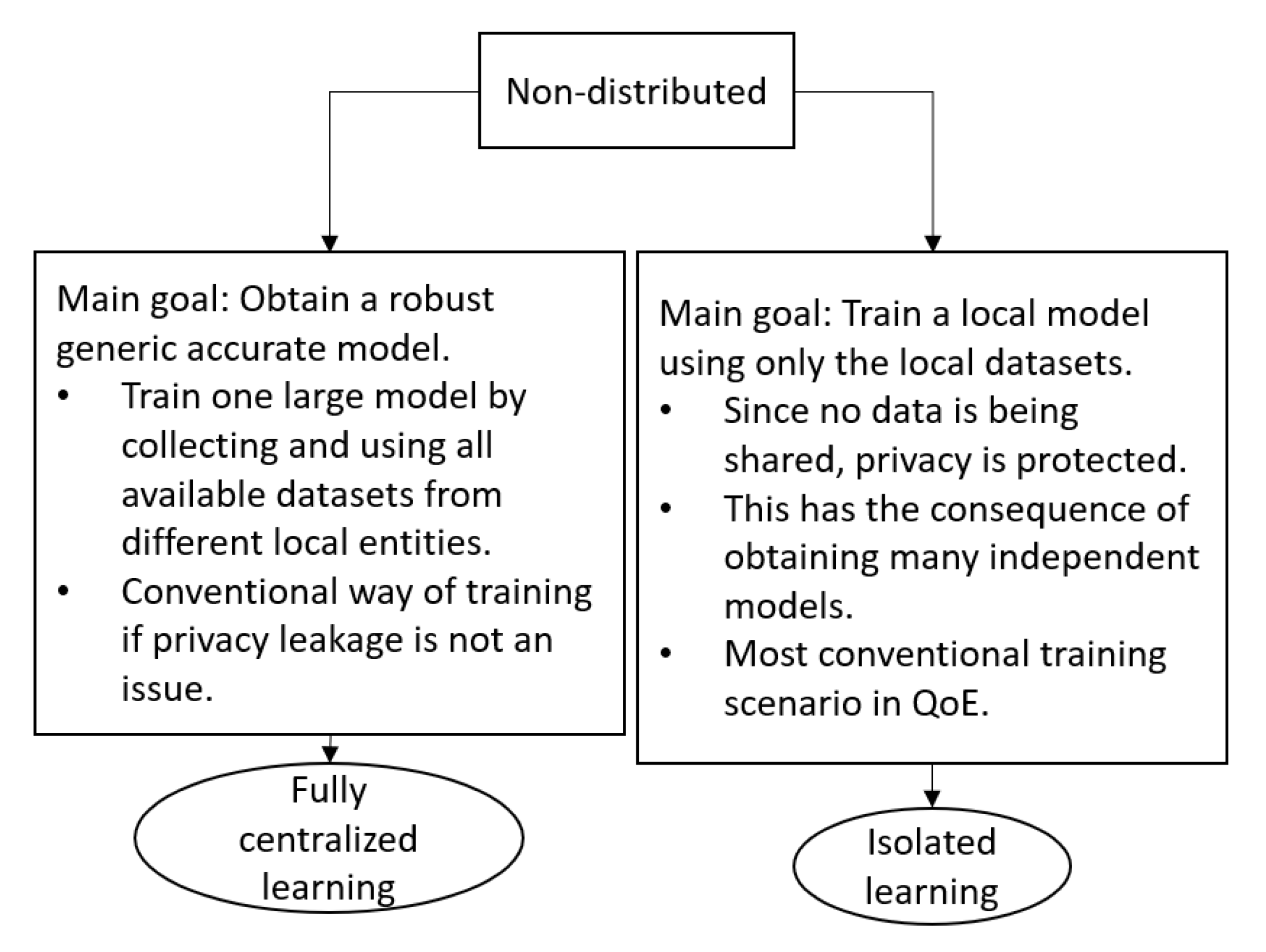
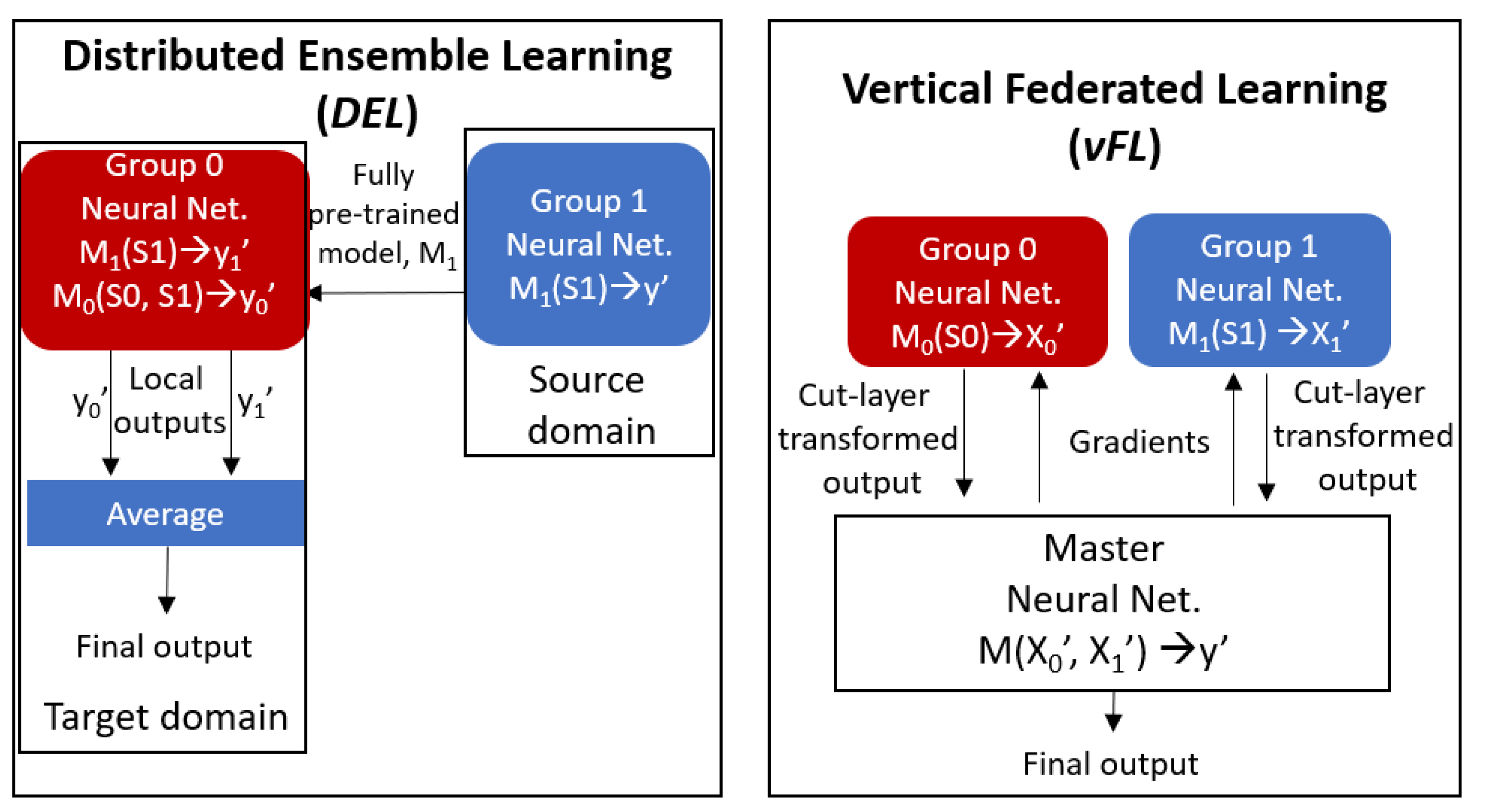
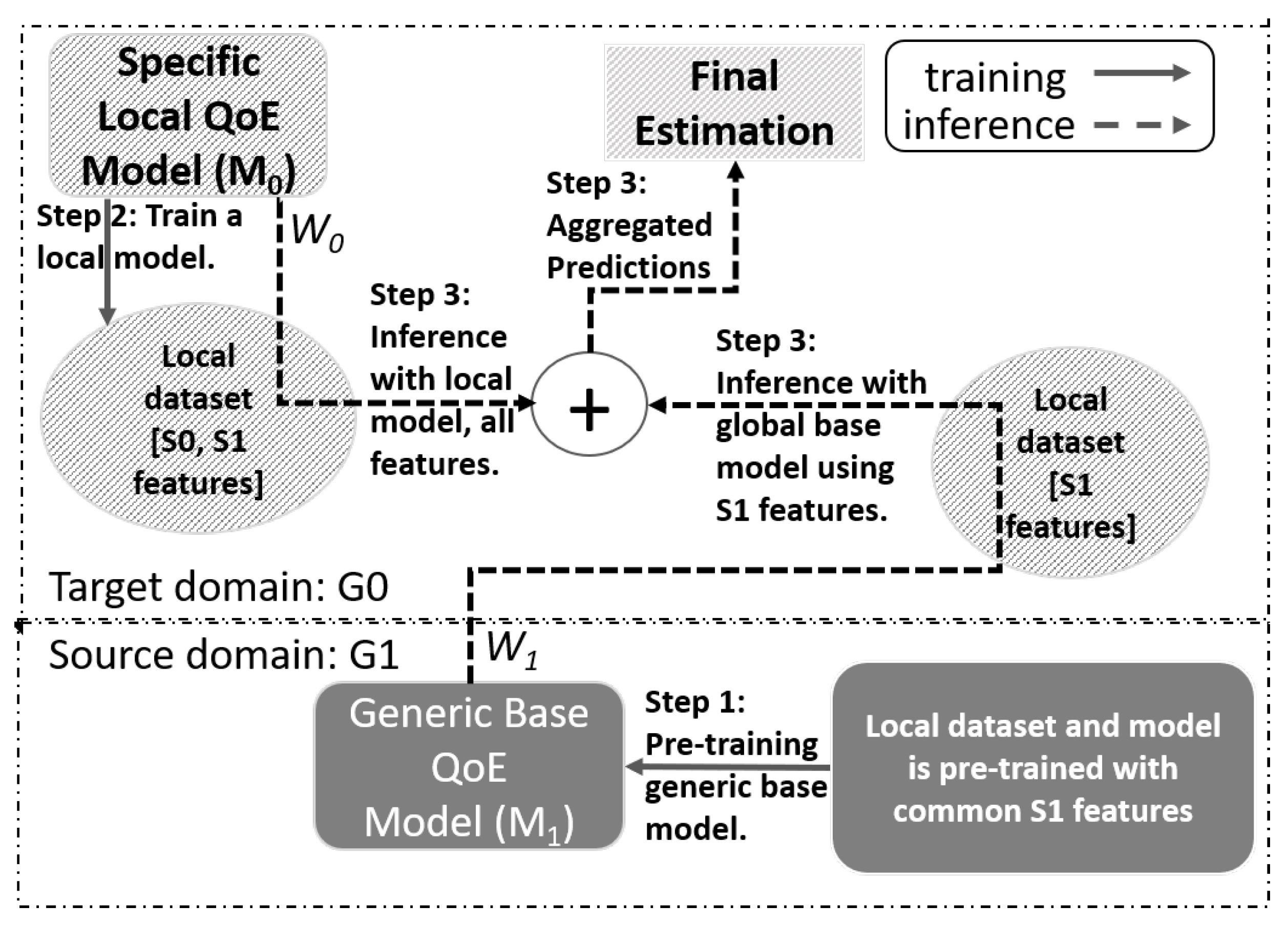
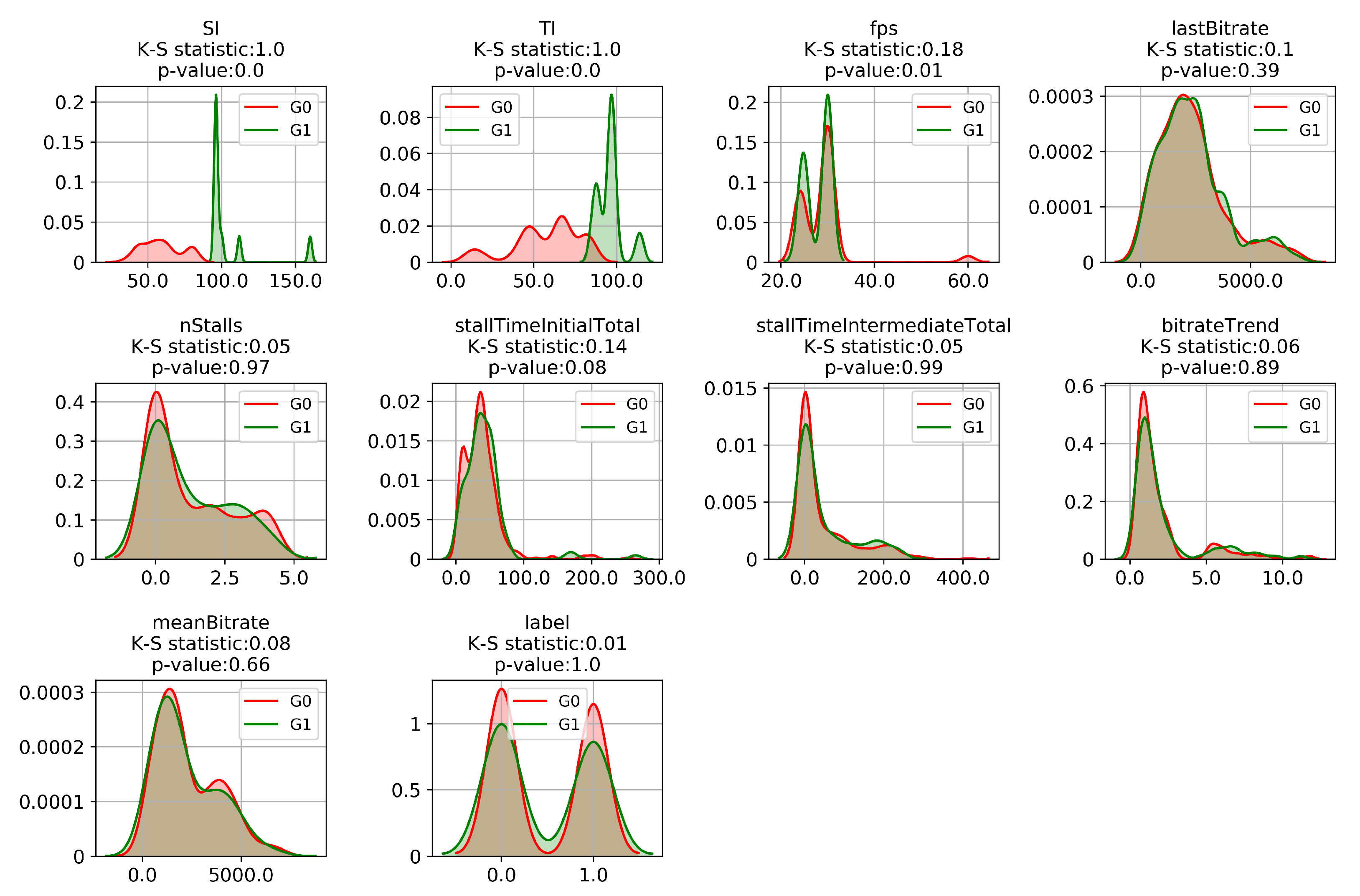
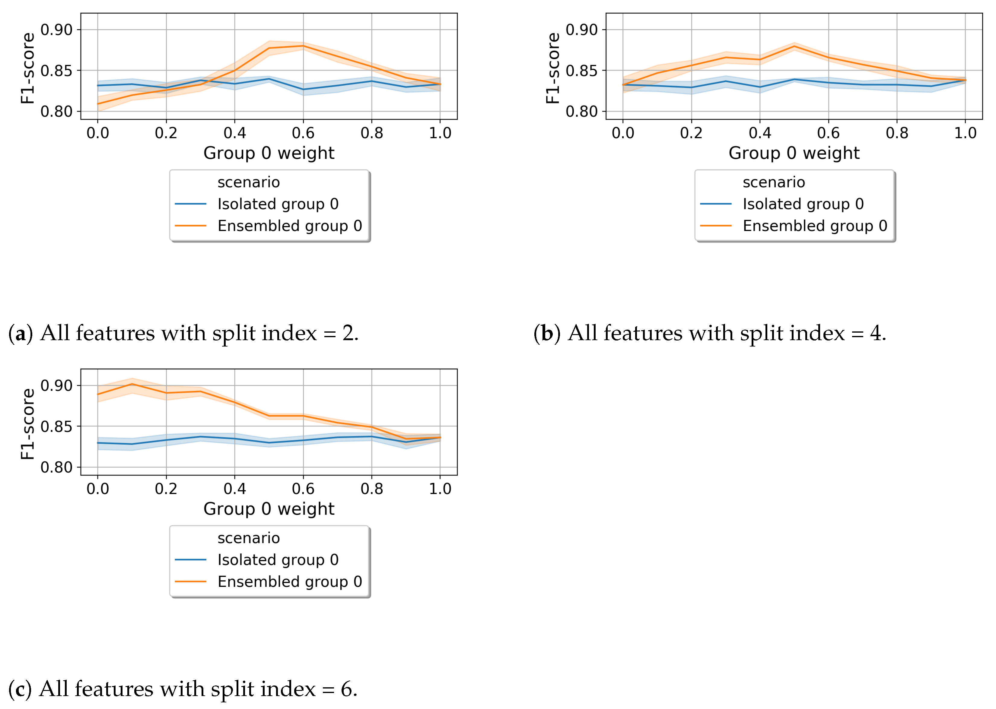
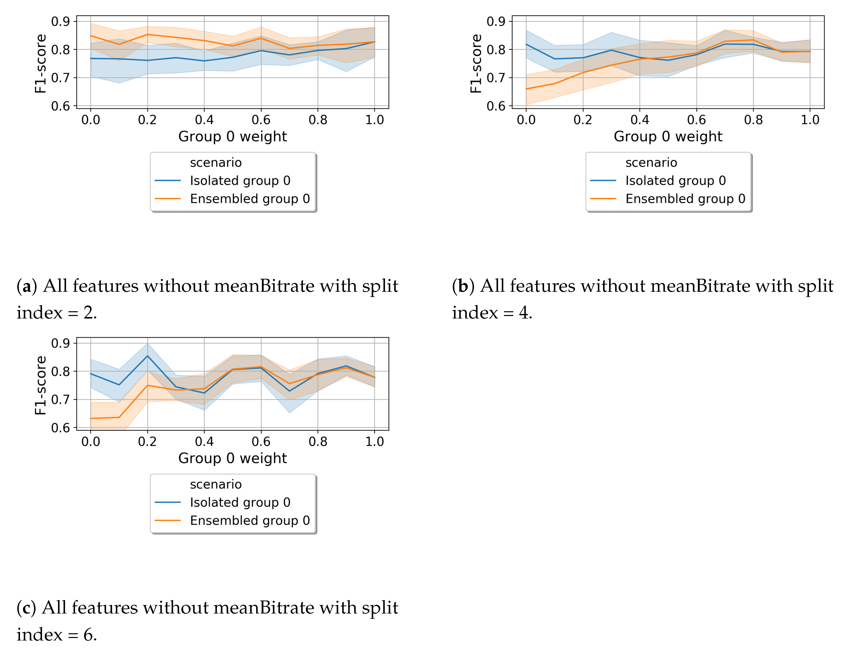
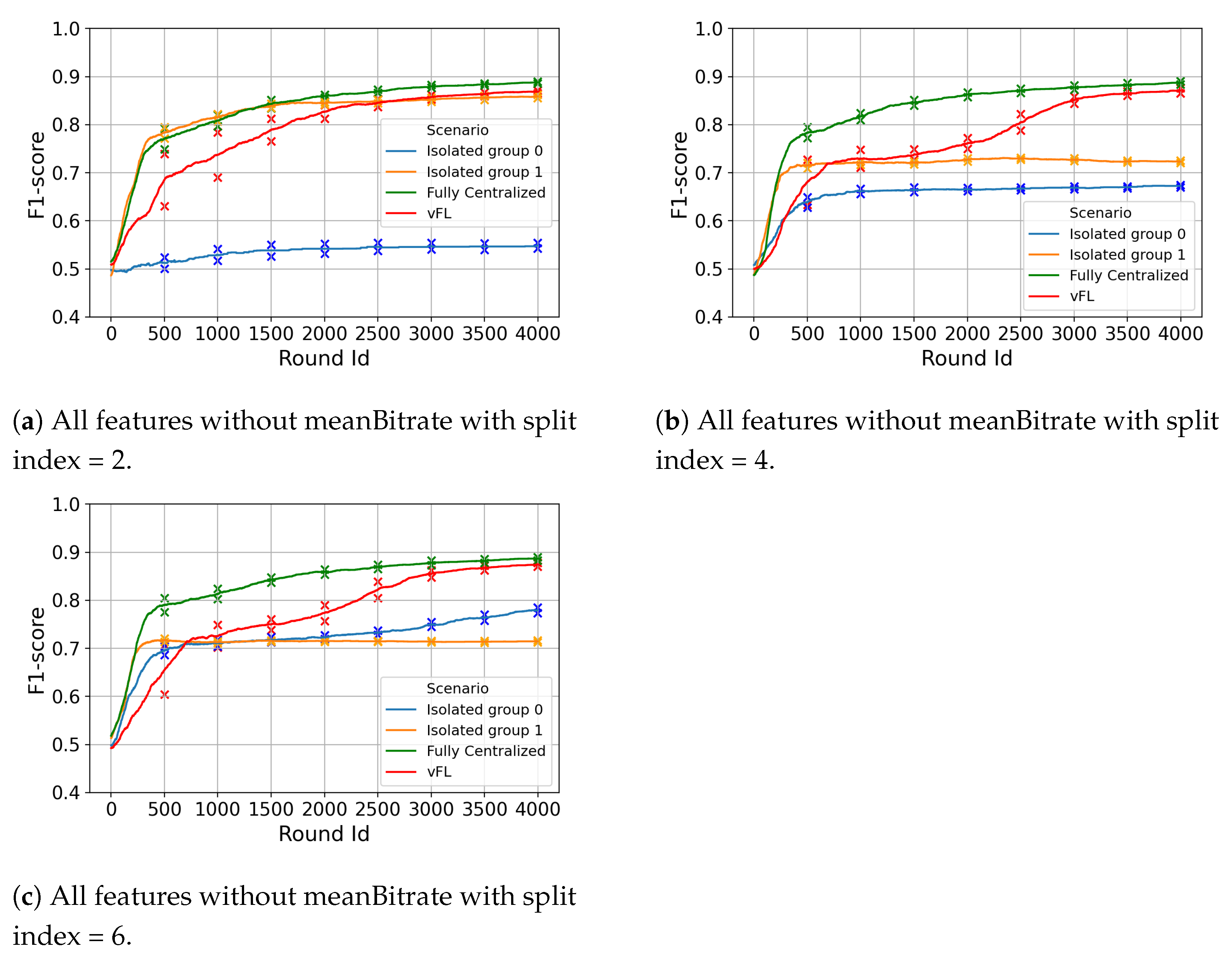
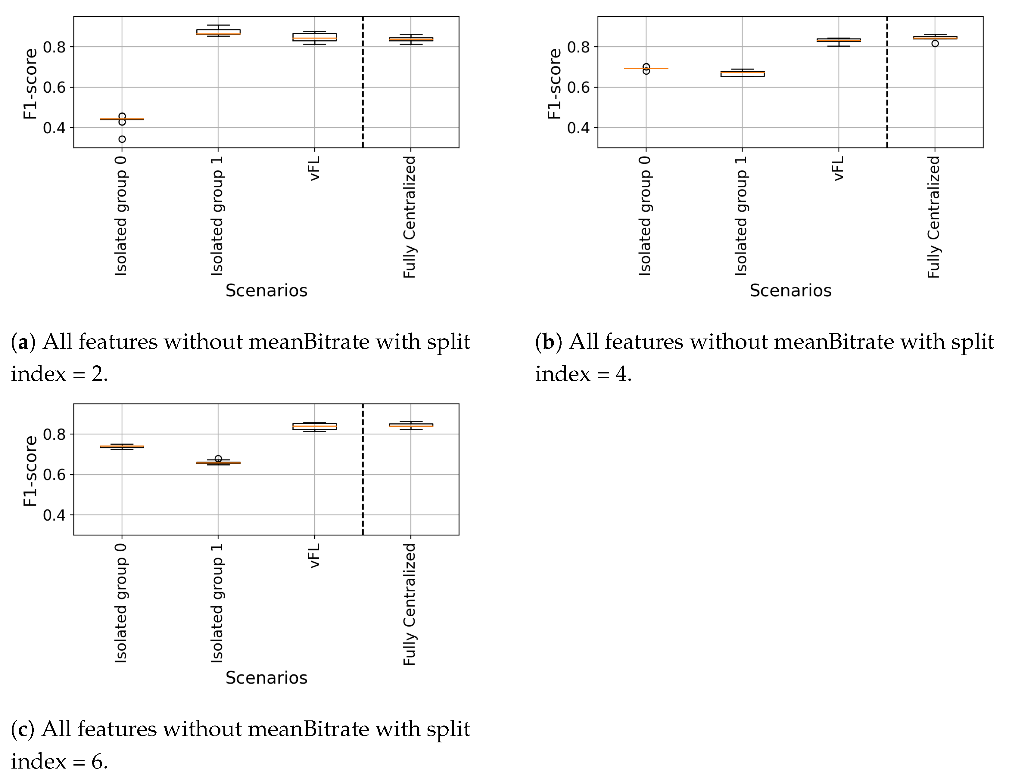
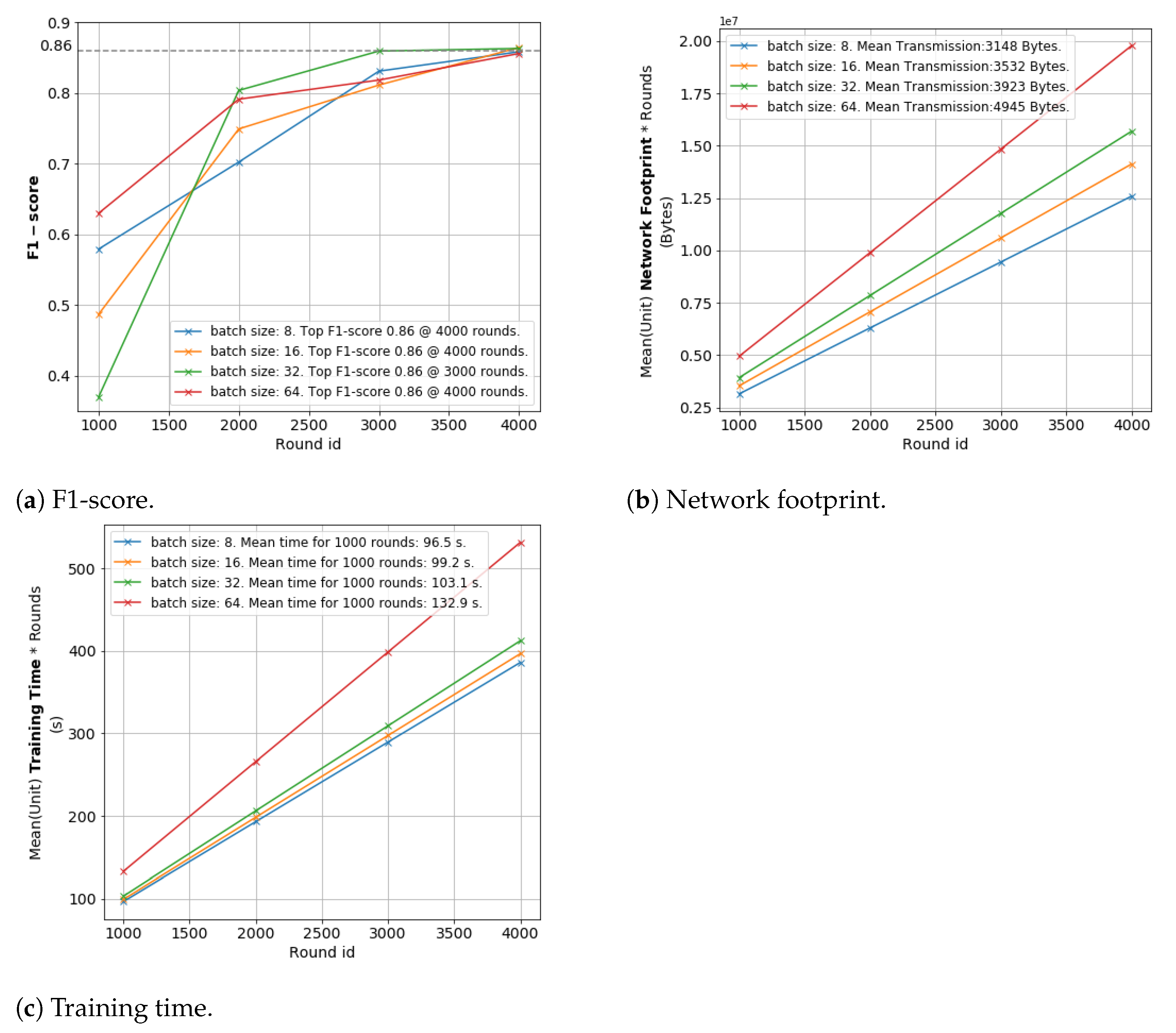
Table 1.
Descriptions of the extracted features for the QoE models, where the Mean Opinion Score (MOS) is the target variable of the model.
Table 1.
Descriptions of the extracted features for the QoE models, where the Mean Opinion Score (MOS) is the target variable of the model.
| Split Index | Feature | Description |
|---|---|---|
| 0 | TI | Video temporal complexity |
| 1 | SI | Video spatial complexity |
| 2 | FPS | Played frames per second |
| 3 | lastbitrate | Last playout bitrate |
| 4 | nstalls | Number of stalls |
| 5 | stallTimeInitialTotal | Initial stalling/buffering duration |
| 6 | stallTimeIntermediateTotal | Total stalling duration |
| 7 | bitrateTrend | Slope of the video playout bitrate |
| 8 | meanBitrate | Average playout bitrate |
| MOS (target variable) | Mean Opinion Score |
Table 2.
Summary of comparison between the distributed learning techniques.
| Technique | Features | What Is Shared? Traffic Direction? | Training Data Location |
|---|---|---|---|
| hFL | All features are same. | Full model. Bidirectional and iteratively. | Input and Output at the same worker. |
| DEL | Target has some source features. | Full model. From Source to Target once. | Input and Output at the same worker. |
| vFL | All features are different. | Cut-layer outputs and gradients. Bidirectional and iteratively. | Input at the workers. Output at the master. |
Table 3.
Average test set F1-score, network footprint, and total training time together with 95% confidence intervals for different neuron counts at the cut-layers of both workers.
Table 3.
Average test set F1-score, network footprint, and total training time together with 95% confidence intervals for different neuron counts at the cut-layers of both workers.
| Neuron Count at the Cut-Layer | F1-Score | Network Footprint [Bytes] | Training Time [s] | ||
|---|---|---|---|---|---|
| Elias ON | Elias OFF | Elias ON | Elias OFF | ||
| 2 | 0.75 ± 0.05 | 5413 ± 3 | 6348 ± 8 | 1472 ± 372 | 1378 ± 150 |
| 4 | 0.85 ± 0.03 | 8102 ± 7 | 10,725 ± 17 | 1161 ± 98 | 1281 ± 122 |
| 8 | 0.86 ± 0.01 | 13,522 ± 11 | 19,087 ± 30 | 1313 ± 24 | 1106 ± 119 |
| 16 | 0.87 ± 0.01 | 23,899 ± 22 | 34,165 ± 48 | 1806 ± 158 | 1624 ± 32 |
| 32 | 0.87 ± 0.01 | 44,602 ± 45 | 66,322 ± 118 | 2885 ± 166 | 1545 ± 114 |
Table 4.
Comparison of different training methodologies.
| Isolated | Fully Centralized | DEL | vFL | |
|---|---|---|---|---|
| Data share | × | ✓ | × | × |
| Model share | × | × | ✓ All-layers | ✓ Cut-layer |
| Sample dep. | × | ✓ | × | ✓ Synch. required |
| Feature dep. | × | ✓ | ✓ Subset | × |
| Jointly train. | × | ✓ | × | ✓ |
| Aggr. | × | × | Average | Concatenate & Split |
| Model agnos. | ✓ | ✓ | ✓ | × Neural Net. |
| Worker contrib. adjustment | N/A | N/A | Manual | Automatic |
| Worker Netw. Footpr. | 0 | |||
| Master Netw. Footpr. | 0 | |||
| Accuracy | Poor | Good | Good | Good |
Publisher’s Note: MDPI stays neutral with regard to jurisdictional claims in published maps and institutional affiliations. |
© 2021 by the authors. Licensee MDPI, Basel, Switzerland. This article is an open access article distributed under the terms and conditions of the Creative Commons Attribution (CC BY) license (https://creativecommons.org/licenses/by/4.0/).
Share and Cite
MDPI and ACS Style
Ickin, S.; Fiedler, M.; Vandikas, K. QoE Modeling on Split Features with Distributed Deep Learning. Network 2021, 1, 165-190. https://0-doi-org.brum.beds.ac.uk/10.3390/network1020011
AMA Style
Ickin S, Fiedler M, Vandikas K. QoE Modeling on Split Features with Distributed Deep Learning. Network. 2021; 1(2):165-190. https://0-doi-org.brum.beds.ac.uk/10.3390/network1020011
Chicago/Turabian StyleIckin, Selim, Markus Fiedler, and Konstantinos Vandikas. 2021. "QoE Modeling on Split Features with Distributed Deep Learning" Network 1, no. 2: 165-190. https://0-doi-org.brum.beds.ac.uk/10.3390/network1020011