
The Frequency Fluctuation Model for the van der Waals Broadening


1
National Research Centre “Kurchatov Institute”, 123182 Moscow, Russia
2
National Research Nuclear University MEPhI, 115409 Moscow, Russia
3
Moscow Institute of Physics and Technology, National Research University, Institutskij Per. 9, 141700 Dolgoprudnyj, Moscow Region, Russia
*
Author to whom correspondence should be addressed.
Foundations 2021, 1(2), 200-207; https://0-doi-org.brum.beds.ac.uk/10.3390/foundations1020015
Submission received: 6 October 2021
/
Revised: 21 October 2021
/
Accepted: 25 October 2021
/
Published: 29 October 2021
(This article belongs to the Special Issue Advances in Fundamental Physics)
Abstract
:The effect of atomic and molecular microfield dynamics on spectral line shapes is under consideration. This problem is treated in the framework of the Frequency Fluctuation Model (FFM). For the first time, the FFM is tested for the broadening of a spectral line by neutral particles. The usage of the FFM allows one to derive simple analytical expressions and perform fast calculations of the intensity profile. The obtained results are compared with Chen and Takeo’s theory (CT), which is in good agreement with experimental data. It is demonstrated that, for moderate values of temperature and density, the FFM successfully describes the effect of the microfield dynamics on a spectral line shape.
1. Introduction
The problem of the microfield dynamics effect on a spectral line shape was recognized many years ago [1,2,3]. There are different methods which were developed to solve this problem [4,5,6]. However, the best agreement with the results of Molecular Dynamics (MD) simulations provides the Frequency Fluctuation Model (FFM) [7]. It is based on dividing a spectral line contour in a static field into separate regions, between which there is an exchange of intensities due to thermal motion. This model is widely used for spectral line shape calculations in plasmas (see, e.g., [8,9,10,11,12,13]). It was shown that the FFM is equivalent to the method of the quantum kinetic Equation [14]. This approach makes it possible to reformulate the FFM in terms of analytical expressions. Namely, the FFM spectral line shape can be considered as the functional of the static profile. This circumstance allows one to use simple analytical expressions and perform fast calculations of a spectral line shape for arbitrary values of temperatures and densities.
The FFM was formulated for spectral line shape calculations in plasmas. It was never used for the Stark broadening by neutral particles—to the best of our knowledge. Most of the material on the van der Waals broadening accumulated by the end of the 1960s is presented in the famous review of S. Chen and M. Takeo [15]. Moreover, in this paper, the authors present the line shape calculation method (based on the work of P.W. Anderson and J.D. Talman [16]) for arbitrary values of temperatures and densities. The Chen and Takeo results (CT) are very old. Nevertheless, they are in good agreement with experimental data and can be used for the examination of the FFM theory. Moreover, the analytical expressions for the line shape presented in [15] are very cumbersome. The direct use of the CT theory in numerical calculations requires significant computational resources. Therefore, the FFM may provide simple analytical expressions for the description of the van der Waals broadening.
The FFM has a drawback. It does not reproduce the impact width correctly. This circumstance was noted in the original paper [7]. Furthermore, it was directly shown in [12,17]. However, this problem was solved for the linear Stark effect. The resolution consists of the dependence of the jumping frequency, which characterizes the rate of change of the microfield on the energy shift. This dependence is obtained by comparing the analytical calculations with MD in the paper [12]. The authors of the work [17] overcame this problem in the alternative way. They used the asymptotic expression of the jumping frequency obtained by S. Chandrasekhar and J. von Neumann [18], who derived this for the description of the stellar dynamics.
The detailed analysis of the FFM results for different plasma parameters is presented in the paper [17]. It is demonstrated that the accounting for the dependence of the jumping frequency on the energy shift leads to the correct behaviour of the spectral line width in the impact limit for the linear Stark effect. The difference between the modified and the original versions of the FFM for moderate values of temperatures and densities is insignificant. Therefore, accounting for the jumping frequency dependence on the field strength yields the simple analytical theory which provides the correct results for a wide range of plasma parameters. The situation is more complicated for the quadratic Stark effect. In this case, the problem of reproducing the impact width is not solved in this way. However, for realistic plasma parameters, the FFM with the constant jumping frequency provides quite satisfactory results.
Usually, the van der Waals broadening can be described in terms of the impact approximation [19]. Furthermore, there are modern works related to the spectral line broadening by neutral atoms and molecules (see, e.g., [20,21]). Therefore, the main goal of the present paper is the examination of the FFM for the van der Waals interaction. The second aim of this work is to provide the simple analytical algorithm for the line shape calculations for low temperatures (less that 300 K) or high densities.
2. Description of the Method
In the present paper, we focused on the spectral broadening by neutral atoms and molecules. The detailed description of the analytical FFM formulation and the discussion of the dynamics effect on the spectral line formation are given in [17]. For convenience, an abridged version was presented below.
The effect of a multiparticle electric field on molecular and atomic spectra is characterized by the ratio of the jumping frequency and the Stark shift:
where
Here, N and are, respectively, the density and the thermal velocity of interacting particles; is the constant of the Stark effect; is called the jumping frequency. The potential of binary interacting particles has the following form:
In the present paper we considered the case of , which corresponds to a wide class of van der Waals interactions. The interaction between atoms and molecules often defers from (4). However, we focused on the examination of the FFM by the comparison with CT results, which were obtained for the potential (4).
The transition from binary to non-binary type of interactions is often characterized by the number of particles is the Weisskopf sphere h. For in Expression (4), it equals to [19]
Parameter (5) also determines the transition from the static theory to the impact limit. The number of particles in the Weisskopf sphere is connected with by the simple relation
Using the results from [19], we could estimate the parameter . For K, approximately equals to:
where N is expressed in cm.
All over the paper, atomic units were used (, where: e—the elementary charge; m—the mass of an electron; ℏ is the Planck constant). Furthermore, for the sake of simplicity, we used the reduced detuning: .
The FFM procedure is equivalent to the method of the kinetic equation with strong-collision integral, which describes an intensity exchange between different regions of a static profile [14]. The frequency of the exchange equals to . The solution of this equation led to the following expression for the resulting profile:
where is the normalized static profile. Note, that when , turns into .
There is a useful relation between the functions and :
S. Chen and M. Takeo presented the analytical expression for the intensity profile for an arbitrary value of for the van der Waals broadening [15]:
where
The function can be approximated by the simple functions:
where is the gamma function.
Expression (12) turned into the static profile when approached zero. In order to derive , it was necessary to use the approximation for for small values of x.
Using the first relation of (13) and the stationary phase approximation, one obtains the following formula for the static profile:
The examination of the FFM consisted of the comparison of the CT Formula (12) with Expression (9). In the integrand of (10), we substituted the static profile (14). In the impact limit (), we could perform a simple estimation of the impact width. Namely, for large values of , the spectral line shape turned into the Lorentzian:
where is the width of the profile and is the coordinate of the centre of the Lorentz profile.
Note, that the CT theory reproduced the impact limit. Indeed, the usage of the second relation from (13) led to Expression (15).
In order to estimate the impact width for the FFM, we used the following property of a wide class of normalized profiles:
Relation (16) was valid here, because in the impact limit, and always have the same dependence on (see, e.g., [19]). Therefore, it was obvious that Property (16) worked for the Lorentz profile (15). Using the asymptotic behaviour of Formula (14), we could estimate :
From Relations (16) and (17), it was easy to see that . Thus, the FFM did not reproduce the behaviour of the profile width in the impact limit. Indeed, it was the well-know result of the impact theory [19], which was . The difference in the dependence of the impact width on the power of velocity was very small .
3. The Results of Numerical Calculations
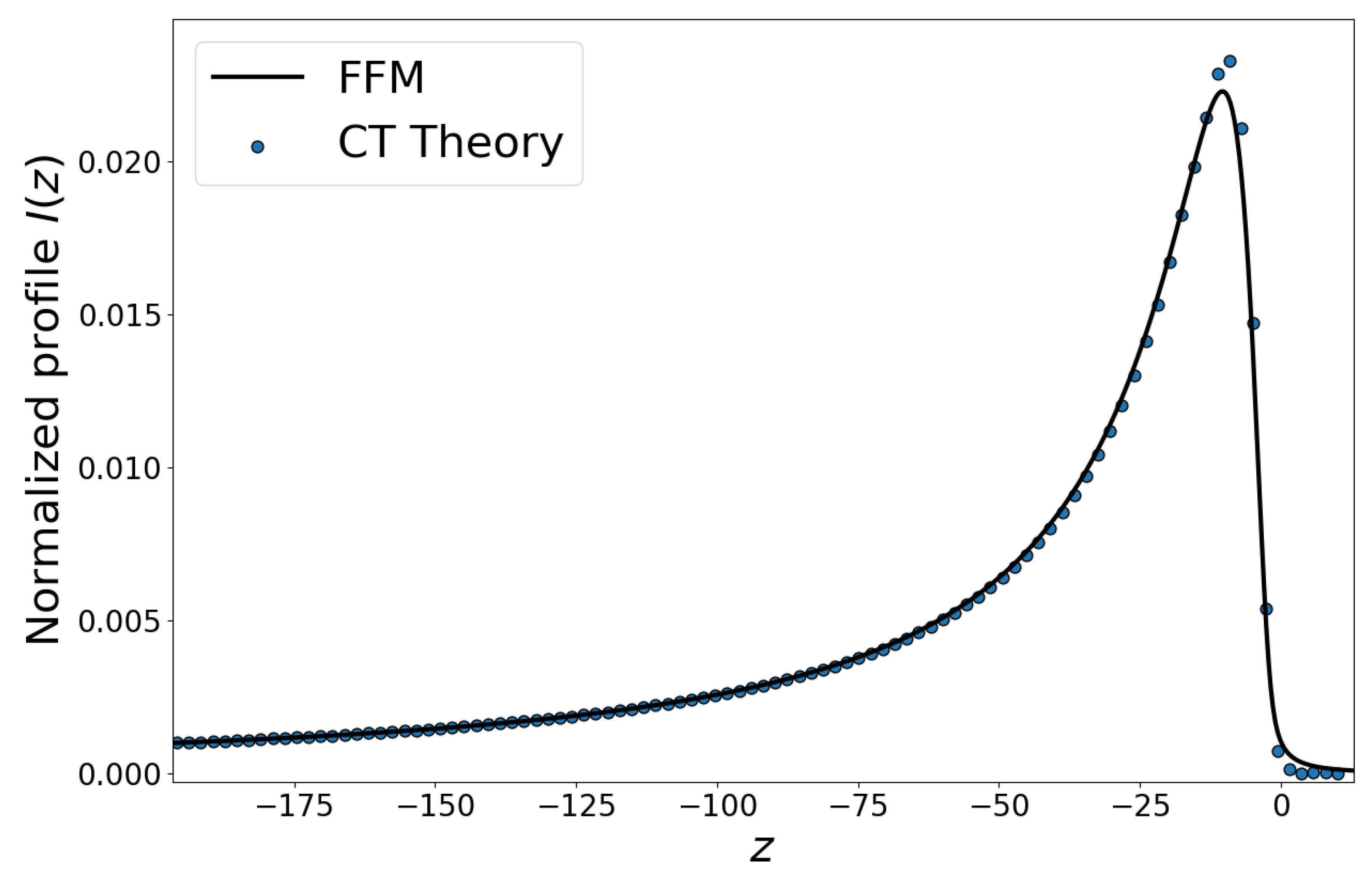
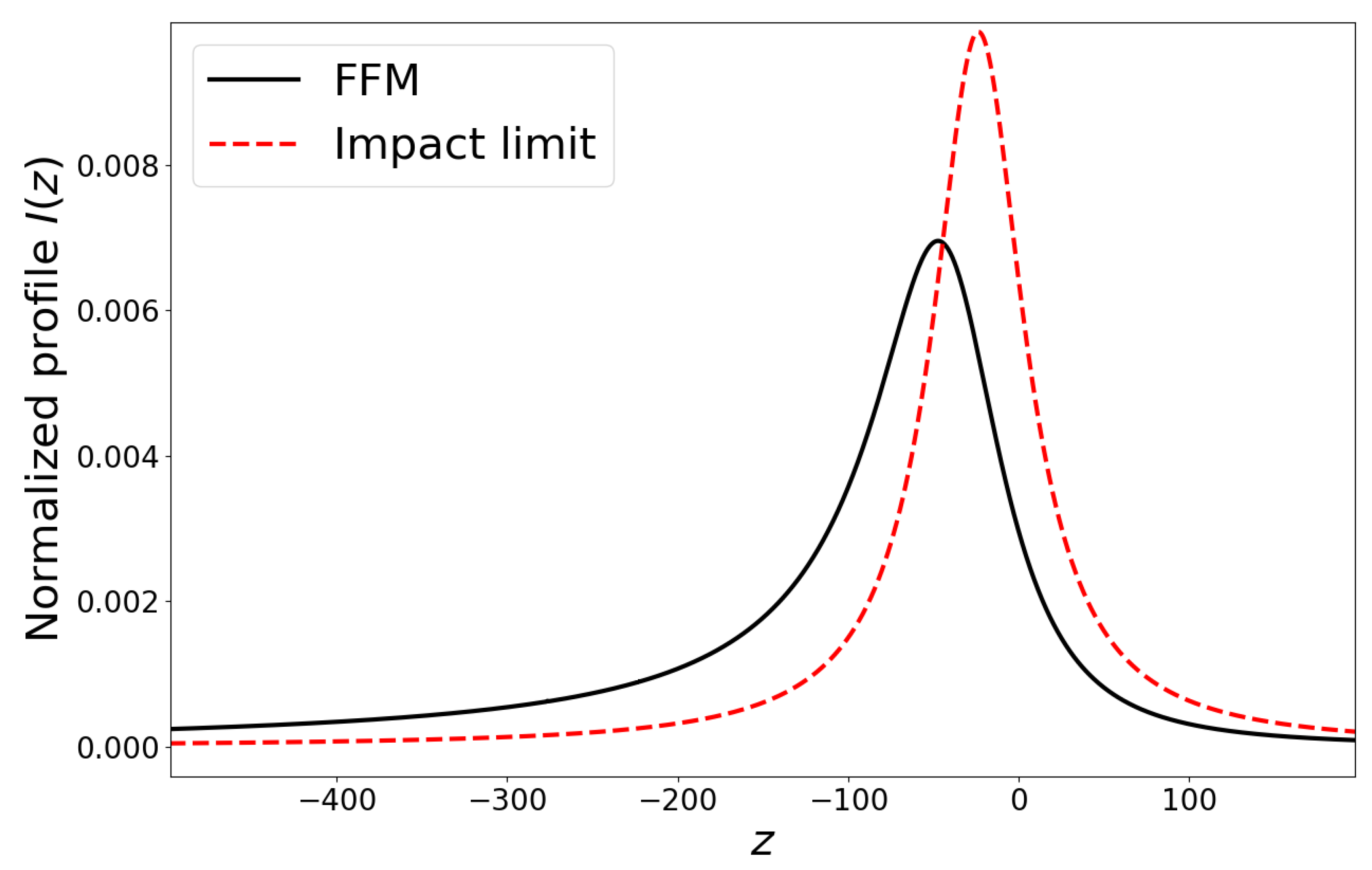
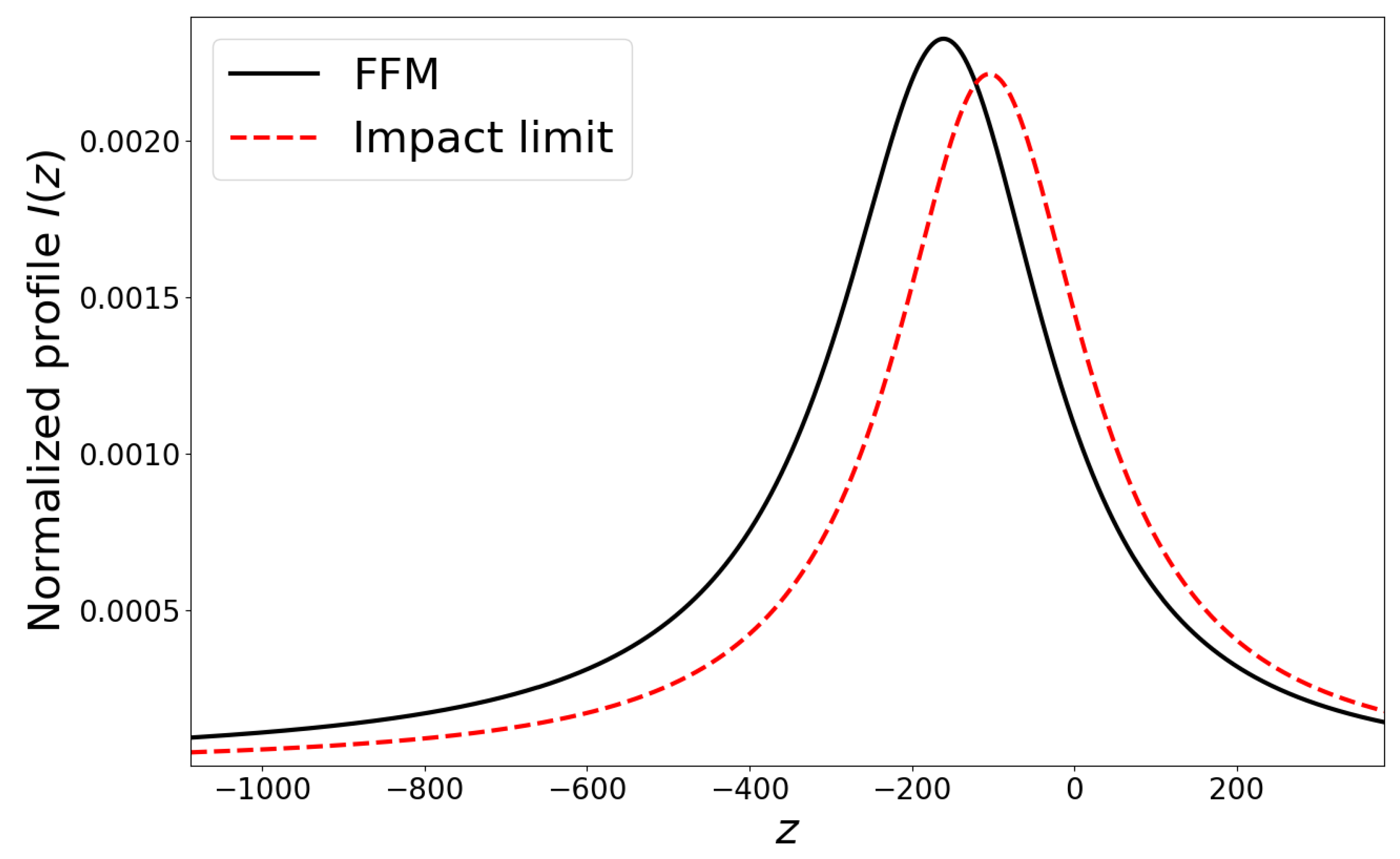
In order to test the FFM procedure, we compared it with the CT results. The numerical calculations showed that, for , the FFM was in good agreement with CT. The example of it is demonstrated in Figure 1, where one can see the comparison of two theories for . However, the FFM did not reproduce the impact width correctly (Figure 2) as it was shown in the previous section by the analytical estimations. The comparison of the CT theory (in the impact limit) with the FFM profile is presented in Figure 2. The full width at half maximum of the FFM profile was approximately 1.5 as large as the impact width for . With an increase in the parameter , the FFM profile slowly became wider than the impact line shape. This circumstance was connected with the slow growth of the ratio: . Moreover, we only knew how depended on . Uncertainty in the value of the prefactor played an important role in the impact width determination. However, the derivation of the certain value of the FFM impact width prefactor by analytical calculations is a complex problem. It might be determined numerically as in the work of [17], but it is not reasonable to do so until the dependence of the jumping frequency on the detuning is determined. The discrepancy between two graphs became insignificant for (Figure 3). According to Estimation (7), this value of for –5000 K corresponded to – cm.
The discrepancy in the impact limit might have most likely been eliminated by accounting for the dependence of the jumping frequency on the detuning. It was shown that, for the linear Stark effect, it led to the correct result for large values of [17]. However, in order to determine this dependence, it was necessary to describe complicated dynamics of the van der Waals forces.
4. Conclusions
The construction of the general analytical theory, which described the effect of the complicated microfield dynamics on the spectral line shape formation, faced the greatest difficulties. The Frequency Fluctuation Model is believed to be the most accurate and simplest method for account such effects. Therefore, it was necessary to examine this theory for different types of interactions. In the present paper, we tested the FFM for the van der Waals forces.
The FFM showed good results for moderate values of temperature and density. In the case of broadening by neutral atoms, it was no exception. The results of the FFM procedure were in agreement with the CT theory (Figure 1).
The FFM did not reproduce the impact width correctly (Figure 2). As it was shown in [17], for the linear Stark effect, this problem could be solved by accounting for the dependence of the jumping frequency on the field strength. Apparently, the resolution of the problem of the broadening by neutral particles consisted of the description of the complicated dynamics of the van der Waals field.
Author Contributions
Conceptualization, V.L., V.A. and A.L.; methodology, V.L.; software, A.L.; validation, V.L., A.L. and V.A.; formal analysis, V.L., V.A. and A.L.; investigation, A.L., V.A. and V.L.; resources, A.L.; data curation, V.L.; writing—original draft preparation, A.L.; writing—review and editing, V.L.; visualization, A.L.; supervision, V.L.; project administration, V.L. All authors have read and agreed to the published version of the manuscript.
Funding
This research received no external funding.
Institutional Review Board Statement
Not applicable.
Informed Consent Statement
Not applicable.
Conflicts of Interest
The authors declare no conflict of interest.
Abbreviations
The following abbreviations are used in this manuscript:
| FFM | Frequency Fluctuation Model |
| MD | Molecular Dynamics |
| CT | Chen and Takeo |
References
- Griem, H.; Baranger, M.; Kolb, A.; Oertel, G. Stark broadening of neutral helium lines in a plasma. Phys. Rev. 1962, 125, 177. [Google Scholar] [CrossRef]
- Kogan, V. Broadening of spectral lines in high-temperature plasma. Plasma Phys. Probl. Control Fusion 1958, 4, 305. [Google Scholar]
- Stambulchik, E.; Maron, Y. Plasma line broadening and computer simulations: A mini-review. High Energy Density Phys. 2010, 6, 9–14. [Google Scholar] [CrossRef]
- Brissaud, A.; Frisch, U. Theory of Stark broadening—II exact line profile with model microfield. J. Quant. Spectrosc. Radiat. Transf. 1971, 11, 1767–1783. [Google Scholar] [CrossRef]
- Alexiou, S. Implementation of the Frequency Separation Technique in general lineshape codes. High Energy Density Phys. 2013, 9, 375–384. [Google Scholar] [CrossRef]
- Ferri, S.; Calisti, A.; Mossé, C.; Rosato, J.; Talin, B.; Alexiou, S.; Gigosos, M.A.; González, M.A.; González-Herrero, D.; Lara, N.; et al. Ion Dynamics Effect on Stark-Broadened Line Shapes: A Cross-Comparison of Various Models. Atoms 2014, 2, 299–318. [Google Scholar] [CrossRef]
- Talin, B.; Calisti, A.; Godbert, L.; Stamm, R.; Lee, R.; Klein, L. Frequency-fluctuation model for line-shape calculations in plasma spectroscopy. Phys. Rev. A 1995, 51, 1918. [Google Scholar] [CrossRef] [PubMed]
- Mossé, C.; Calisti, A.; Stamm, R.; Talin, B.; Bureyeva, L.; Lisitsa, V. A universal approach to Rydberg spectral line shapes in plasmas. J. Phys. At. Mol. Opt. Phys. 2004, 37, 1343. [Google Scholar] [CrossRef]
- Calisti, A.; Bureyeva, L.; Lisitsa, V.; Shuvaev, D.; Talin, B. Coupling and ionization effects on hydrogen spectral line shapes in dense plasmas. Eur. Phys. J. D 2007, 42, 387–392. [Google Scholar] [CrossRef]
- Calisti, A.; Mossé, C.; Ferri, S.; Talin, B.; Rosmej, F.; Bureyeva, L.; Lisitsa, V. Dynamic Stark broadening as the Dicke narrowing effect. Phys. Rev. E 2010, 81, 016406. [Google Scholar] [CrossRef] [PubMed]
- Ferri, S.; Calisti, A.; Mossé, C.; Mouret, L.; Talin, B.; Gigosos, M.A.; González, M.A.; Lisitsa, V. Frequency-fluctuation model applied to Stark-Zeeman spectral line shapes in plasmas. Phys. Rev. E 2011, 84, 026407. [Google Scholar] [CrossRef] [PubMed]
- Stambulchik, E.; Maron, Y. Quasicontiguous frequency-fluctuation model for calculation of hydrogen and hydrogenlike Stark-broadened line shapes in plasmas. Phys. Rev. E 2013, 87, 053108. [Google Scholar] [CrossRef] [PubMed] [Green Version]
- Letunov, A.; Lisitsa, V. The Coulomb Symmetry and a Universal Representation of Rydberg Spectral Line Shapes in Magnetized Plasmas. Symmetry 2020, 12, 1922. [Google Scholar] [CrossRef]
- Bureeva, L.; Kadomtsev, M.; Levashova, M.; Lisitsa, V.; Calisti, A.; Talin, B.; Rosmej, F. Equivalence of the method of the kinetic equation and the fluctuating-frequency method in the theory of the broadening of spectral lines. JETP Lett. 2010, 90, 647–650. [Google Scholar] [CrossRef]
- Takeo, M.; Chen, S. Broadening and shift of spectral lines due to the presence of foreign gases. Rev. Mod. Phys. 1957, 29, 20. [Google Scholar]
- Anderson, P.; Talman, J. Proceedings of the Conference on Broadening of Spectral Lines, Murray Hill, NJ, USA, 3 May 1956.
- Astapenko, V.; Letunov, A.; Lisitsa, V. From the Vector to Scalar Perturbations Addition in the Stark Broadening Theory of Spectral Lines. Universe 2021, 7, 176. [Google Scholar] [CrossRef]
- Chandrasekhar, S.; von Neumann, J. The Statistics of the Gravitational Field Arising from a Random Distribution of Stars. Astrophys. J. 1942, 95, 489–531. [Google Scholar] [CrossRef] [Green Version]
- Sobelman, I.I. Introduction to the Theory of Atomic Spectra: International Series of Monographs in Natural Philosophy; Elsevier: Amsterdam, The Netherlands, 2016; Volume 40. [Google Scholar]
- Demura, A.; Umanskii, S.Y.; Scherbinin, A.V.; Zaitsevskii, A.V.; Demichenko, G.V.; Astapenko, V.A.; Potapkin, B.V. Evaluation of Van der Waals Broadening Data. Int. Rev. At. Mol. Phys. 2011, 2, 109–150. [Google Scholar]
- Omar, B.; González, M.Á.; Gigosos, M.A.; Ramazanov, T.S.; Jelbuldina, M.C.; Dzhumagulova, K.N.; Zammit, M.C.; Fursa, D.V.; Bray, I. Spectral line shapes of He I line 3889 Å. Atoms 2014, 2, 277–298. [Google Scholar] [CrossRef] [Green Version]
- Margenau, H. Theory of pressure effects of foreign gases on spectral lines. Phys. Rev. 1935, 48, 755. [Google Scholar] [CrossRef]
Figure 1.
The normalized intensity profile of one spectral component as the function of the reduced energy shift. Comparison of the FFM profile with the Chen and Takeo theory; .
Figure 1.
The normalized intensity profile of one spectral component as the function of the reduced energy shift. Comparison of the FFM profile with the Chen and Takeo theory; .

Figure 2.
The normalized intensity profile of one spectral component as the function of the reduced energy shift. Comparison of the FFM profile with the impact theory; .
Figure 2.
The normalized intensity profile of one spectral component as the function of the reduced energy shift. Comparison of the FFM profile with the impact theory; .

Figure 3.
The normalized intensity profile of one spectral component as the function of the reduced energy shift. Comparison of the FFM profile with the impact theory; .
Figure 3.
The normalized intensity profile of one spectral component as the function of the reduced energy shift. Comparison of the FFM profile with the impact theory; .

Publisher’s Note: MDPI stays neutral with regard to jurisdictional claims in published maps and institutional affiliations. |
© 2021 by the authors. Licensee MDPI, Basel, Switzerland. This article is an open access article distributed under the terms and conditions of the Creative Commons Attribution (CC BY) license (https://creativecommons.org/licenses/by/4.0/).
Share and Cite
MDPI and ACS Style
Letunov, A.; Lisitsa, V.; Astapenko, V. The Frequency Fluctuation Model for the van der Waals Broadening. Foundations 2021, 1, 200-207. https://0-doi-org.brum.beds.ac.uk/10.3390/foundations1020015
AMA Style
Letunov A, Lisitsa V, Astapenko V. The Frequency Fluctuation Model for the van der Waals Broadening. Foundations. 2021; 1(2):200-207. https://0-doi-org.brum.beds.ac.uk/10.3390/foundations1020015
Chicago/Turabian StyleLetunov, Andrei, Valery Lisitsa, and Valery Astapenko. 2021. "The Frequency Fluctuation Model for the van der Waals Broadening" Foundations 1, no. 2: 200-207. https://0-doi-org.brum.beds.ac.uk/10.3390/foundations1020015