
Multidimensional Dominance Drawings and Their Applications

1
Department of Electronic and Information Engineering, University of Perugia, 06123 Perugia, Italy
2
Computer Science Department, University of Crete, 70013 Heraklion, Greece
*
Author to whom correspondence should be addressed.
Foundations 2021, 1(2), 271-285; https://0-doi-org.brum.beds.ac.uk/10.3390/foundations1020020
Submission received: 28 July 2021
/
Revised: 1 November 2021
/
Accepted: 10 November 2021
/
Published: 24 November 2021
(This article belongs to the Section Information Sciences)
Abstract
:In a dominance drawing of a directed acyclic graph (DAG) G, a vertex v is reachable from a vertex u if, and only if all the coordinates of v are greater than or equal to the coordinates of u in . Dominance drawings of DAGs are very important in many areas of research. They combine the aspect of drawing a DAG on the grid with the fact that the transitive closure of the DAG is apparently obvious by the dominance relation between grid points associated with the vertices. The smallest number d for which a given DAG G has a d-dimensional dominance drawing is called dominance drawing dimension, and it is NP-hard to compute. In this paper, we present efficient algorithms for computing dominance drawings of G with a number of dimensions respecting theoretical bounds. We first describe a simple algorithm that shows how to compute a dominance drawing of G from its compressed transitive closure. Next, we describe a more complicated algorithm, which is based on the concept of modular decomposition of G, and obtaining dominance drawings with a lower number of dimensions. Finally, we consider the concept of weak dominance, a relaxed version of the dominance, and we discuss interesting experimental results.
1. Introduction
Dominance drawings of directed acyclic graphs (DAGs) are very important in many areas of research, including graph drawing [1], computational geometry [2], and information visualization [3], even in very large databases [4], just to mention a few. They combine the aspect of drawing a DAG on the grid with the fact that the transitive closure of the DAG is apparently obvious by the dominance relation between grid points associated with the vertices. In other words, in a dominance drawing, a vertex v is reachable from a vertex u if, and only if all the coordinates of v are greater than or equal to the coordinates of u in . Notice that it is not possible to find dominance drawings in two-dimensions for most DAGs. The smallest number d for which a given DAG G has a d-dimensional dominance drawing is called a dominance drawing dimension, and it is NP-hard to compute [5]. We denote by the dominance drawing dimension of G. In this paper, we present algorithms for computing a k-dimensional dominance drawing of G, where . Our algorithms are efficient and based on various decomposition techniques.
An -graph is a DAG with one source s and one sink t. Every DAG can be transformed into an -graph by adding a virtual source and connecting it to all the sources and by adding a virtual sink and connecting all the sinks to it. In this paper, we assume, without loss of generality, that every DAG is an -graph. Let be an -graph. There are linear-time algorithms for computing two-dimensional dominance drawings of -graphs that are planar (-planar graphs) [6]. For non-planar -graphs, more than two dimensions are usually required. A k-dimensional () drawing of G is a drawing of G having k dimensions that we denote by . For every and , is the coordinate in the dimension of v. In a k-dimensional dominance drawing of G, given any two vertices , for every if, and only if there exists a directed path connecting u to v in G. In this paper, we assume that every path is a directed path. Hence, from now on we omit the word “directed”.
The minimum k such that there exist a k-dimensional dominance drawing of G (its dominance dimension) is . A partially ordered set (poset) is a mathematical formalization of the concept of ordering. Any partially ordered set P can be viewed as a transitive DAG. The dimension of a poset is equivalent to the dominance dimension of the corresponding -graph and the results obtained for -graphs and their dominance drawing dimension transfer directly to partial orders and their dimension, and vice versa (see [5] for a formal definition of poset and dimension of a poset). Hence, it follows that we can talk about the known results for partial orders and for -graphs with no distinction.
Testing whether an -graph has a dominance dimension of two requires linear time [7,8]. In particular, [7] gives a necessary and sufficient condition for the test, and [8] presents the linear-time algorithm. It is NP-complete to decide whether is greater than or equal to 3 [5]. A linear-time algorithm that constructs two-dimensional dominance drawings of upward planar graphs is described in [2] (see also [6]). We report the above results in the following lemma:
Lemma 1.
Given a k-dimensional dominance drawing of a DAG G, it is possible to test the existence of a path connecting any two vertices of G in time. DAGs are used to represent information in databases. Computing dominance drawings of such DAGs having a low number of dimensions would be important in practice. Unfortunately, most of the existing algorithms for constructing dominance drawings require the input DAG to have specific properties, for example, to be planar, as stated in Lemma 1. For this reason, a relaxed version of dominance drawing, called weak dominance drawing, was introduced in [9]. The “if and only if” condition of dominance becomes an “if” condition in the weak dominance. This implies that the non-existence of a path between the two vertices is guaranteed by finding a dimension D for which , but the existence of a path is not guaranteed even if for all dimensions D of . Hence, there is a falsely implied path (fip) between u and v when there is no path between u and v, even though for every dimension D of . The existence of fips cannot be excluded since the number of dimensions in a weak dominance drawing is typically significantly less than .
Li, Hua, and Zhou considered high-dimensional weak dominance drawings in order to obtain efficient solutions to the reachability query problem [10]. Their experimental results show that their algorithms compute weak dominance drawings using few dimensions and having few fips. Extending their work, Lionakis et al. [11] showed that, for the same families of graphs considered in [10] and by using a number of dimensions similar to the one used in [10], it is possible to compute dominance drawings (i.e., 0 fips).
The technique used in [11] is similar to the one described in Section 2 of this paper. The computational time required to compute dominance drawings in [11] is still higher than the one to compute weak dominance drawings [10]. However, these results suggest that a possible direction for this line of research is to actually use directly dominance drawings instead of weak dominance drawings.
This technique is based on the concept of compressed transitive closure, which is a data structure introduced in [12] that can be used to answer any reachability query in and requires space, where k is a parameter less than or equal to n.
In Section 3, we present algorithms that compute dominance drawings with a reduced number of dimensions, k, and show that k is a good upper bound of the dominance dimension number of a DAG. These algorithms are based on a clever decomposition of a DAG denoted by modular decomposition, where a module of a DAG is a set of vertices M of the G having the same set of predecessor and successors in . We also show an interesting family of DAGs for which the number of required dimensions is reduced to a small constant.
Next, we discuss the option of using weak dominance more extensively and close our paper by presenting our conclusions and future research challenges.
2. Compressed Transitive Closure and Dominance Drawings
Let be an -graph with n vertices and m edges. Two vertices are incomparable if there is no path from u to v or from v to u in G. The width of G, denoted by f, is the cardinality of the largest set such that, for every , u and v are incomparable. Given any -graph G, the following lemma describes well-known relationships between its dominance dimension , number of vertices n, and width f.
Lemma 2.
Let G be an -graph, n be its number of vertices, and f be its width. The two following inequalities hold:
Let s and t be the source and sink of G. A chain of G is an ordered set of vertices such that, given any two vertices , u precedes v in the order of C if, and only if there is a path from u to v in G. See, for example, Figure 1a, where and are two chains of G.
Definition 1.
A chain cover of G is a set of chains of G having the following two properties:
- (a)
- is a partition of ;
- (b)
- s and t are contained in every chain of .
An antichain A is a set of vertices such that any pair of vertices is incomparable. Notice that the maximum cardinality of an antichain is equivalent to the width of G. Dilworth [15] proves that the minimum number of chains needed to cover all the vertices of an -graph G is equivalent to the maximum cardinality of the antichain G. We have the following lemma:
Lemma 3.
See Figure 1a, where is a chain cover of graph G. Since , by Lemma 3 is a chain cover of G with minimum cardinality.
For the rest of this paper, we assume that is an -graph and we denote by n, m, and f the number of vertices, the number of edges, and the width of G, respectively. By Inequality (2) of Lemma 2, we have . In this section, we present a simple and efficient algorithm to compute an f-dimensional dominance drawing of G. We first show how to compute a data structure called the compressed transitive closure of G [12], and then we show that this data structure can be easily used to obtain a dominance drawing.
The compressed transitive closure was presented in [12]. Given a chain cover of G of size k, the compressed transitive closure is a set of n arrays of size k, each one associated to a vertex of G. The compressed transitive closure is an efficient tool for answering reachability queries that has low storage requirements and, as we are going to show later, it can be computed in time if a chain cover is given as an input, where k is the cardinality of .
As we are going to observe later, the compressed transitive closure can answer any reachability query in time, and not . Similarly, the dominance drawing described in this section can be used to answer any reachability query in time. We show that if we see every array of the compressed transitive closure as the coordinates of the corresponding vertex of G in an k-dimensional drawing of G, then drawing is a dominance drawing of G.
Given a chain cover of cardinality k, computing the compressed transitive closure requires time. Since computing having cardinality f requires time by Lemma 3, we have that it is possible to compute an f-dimensional dominance drawing of any DAG G in time. To the best of our knowledge, this is the first polynomial-time algorithm to compute a dominance drawing of G in f dimensions.
Let be a chain cover of G. As we said before, we show that the compressed transitive closure of G given can be seen as a k-dimensional dominance drawing of G. Before defining the compressed transitive closure, we introduce some notation. By Property (a) of a chain cover, each vertex v of belongs to exactly one chain, say , of . We denote v by meaning that v is the jth vertex of chain . A similar notation is also used in [12,16]. By Property (b) of a chain cover, s and t belong to every chain of , and we define and for every . An example is shown in Figure 1a. According to this notation, we have: ; ; ; ; ; ; ; .
As we said before, the compressed transitive closure of G given a chain cover of G is a data structure that can answer any reachability query in time that can be computed in time and that requires ) space. More precisely, it is a set of n arrays of integers of size k so that every vertex u of G is assigned to the reachability array , and the following property holds:
Property 1
(Reachability Property [12]). Let u be any vertex of G and be its reachability array. For any vertex of G there exists a directed path from u to v if, and only if .
In other words, vertex is the vertex having the lowest position in so that there is a path from u to . Consequently, there is a path from u to a vertex if, and only if the position q of in is not lower than the position of in . Notice that if , then the directed path exists and it is the empty path and, consequently, .
Figure 1b shows the compressed transitive closure of G given the chain cover shown in Figure 1a. Concerning s and t, we have: and ; , , and . Regarding the other vertices, for example, vertex , we have and . Vertex is the vertex having the lowest position in so that there exists a directed path from to . Additionally, . The value in position 1 of the reachability array of equals the position of in and, consequently, .
We now present the algorithm to compute the compressed transitive closure [12]. The input is an -graph and a chain cover of G. The output is the reachability array for every , that is, the compressed transitive closure of G given . The Algorithm 1 has two steps: the Initialization and the Update.
| Algorithm 1 Compressed transitive closure computation. |
|
Observe that the above algorithm requires time, since, for every vertex of the graph, you compute k operations. See the Step Update 3. We now show that if we use the reachability array as the coordinates of u in a k-dimensional drawing of G for every vertex u, then we obtain a dominance drawing. See Algorithm 2.
| Algorithm 2 CC-Draw (Chain Cover Draw). |
⋆ Input: An -graph and a chain cover of G ⋆ Output: A k-dimensional drawing of G. • Compute the compressed transitive closure of G given . • Compute k-dimensional drawing of G having dimensions such that, for every and for every , . |
We denote by the output of Algorithm 1 when G and are given to the algorithm as an input. Refer to Figure 1. Figure 1c depicts the two-dimensional dominance drawing of G computed by using the chain cover depicted in Figure 1a. The compressed transitive closure of G given is depicted in Figure 1b. For example, and, consequently, and .
Two vertices are placed in the same position in if for every . In a drawing of a graph, two distinct vertices are never placed in the same position by definition. The following lemma shows that two vertices are never placed in the same position in and that, consequently, is a drawing of G.
Lemma 4.
Let be a chain cover of G and let u and v be any two distinct vertices of G. Vertices u and v are not placed in the same position in .
Proof.
Let , , and . Suppose first that u and v belong to the same chain, that is, . In this case, and . In addition, since u and v are two distinct vertices. We have and . It follows that and that, consequently, u and v are not placed in the same position in . Suppose that u and v belong to two distinct chains, that is, . We have , and , . Consider the two vertices and . Suppose by contradiction that the vertices u and v are placed in the same position in . In this case, and and, consequently, and . Hence, and . By the Reachability Property, and are the vertices having the lowest position in and so that there exist a directed path from u to and from v to , respectively. Since and , it follows that there is a path connecting v to u and there is another path connecting u to v. It implies that there must be a cycle that contains v and u in G, which is a contradiction. It follows that u and v are not placed in the same position in . □
Notice that if u and v were placed in the same position, not only could not be considered a drawing of G, but also would not have the property of a dominance drawing. Indeed, in this case and for every and, consequently, the property of the dominance drawing would imply the existence of a path from u to v and a path from v to u and, consequently, the existence of a cycle in G.
The following theorem shows that drawing is a dominance drawing of G and that it can be computed in time.
Theorem 1.
Let G be an -graph with n vertices and m edges and be a chain cover of G. We have that is a k-dimensional dominance drawing of G. Additionally, given a chain cover , can be computed in time.
Proof.
The fact that computing requires time is a direct consequence of the fact that given as input, the compressed transitive closure of G given can be computed in [12]. We now prove that is a k-dimensional dominance drawing of G. Let and be any two distict vertices of G. By Lemma 4u and v are not placed in the same position in . We prove that for every if, and only if there is a path connecting u to v. If for every , then . Since and , we have and, by the Reachability Property, there is a directed path from u to v. It remains to show that if there exists a directed path from u to v then for every . Suppose by contradiction that there exist so that . Since and , we have . We denote by the vertex . Note that by the Reachability Property there is a path connecting v to . Since by hypothesis there is a path from u to v, there is a path connecting u to . On the other hand, since , by the Reachability Property we have that there is no path from u to . A contradiction. Hence, for every . □
By Lemma 3 computing so that requires time. Hence, the following theorem is a consequence of Lemma 3 and Theorem 1.
Theorem 2.
Let G be an -graph with n vertices and m edges and let f be its width. It is possible to compute an f-dimensional dominance drawing of G in time.
3. Transitive Modules and Dominance Drawings
Let G be an -graph. In this section, we first discuss the concept of transitive module of G, which is a module of the transitive graph of G. Second, we present Lemma 5, which shows a bound for not higher than the bounds of Lemma 2. In Section 3.1 we present an algorithm computing dominance drawings respecting the bound of Lemma 5 and in Section 3.2 we discuss its time complexity. The algorithm of Section 2 is simpler than the one described in Section 3.1. On the other hand, as we show in Section 3.3, there exists graph for which the dominance drawings computed by the algorithm of Section 3.1 have less dimensions with respect to the dominance drawings computed by the algorithm of Section 2.
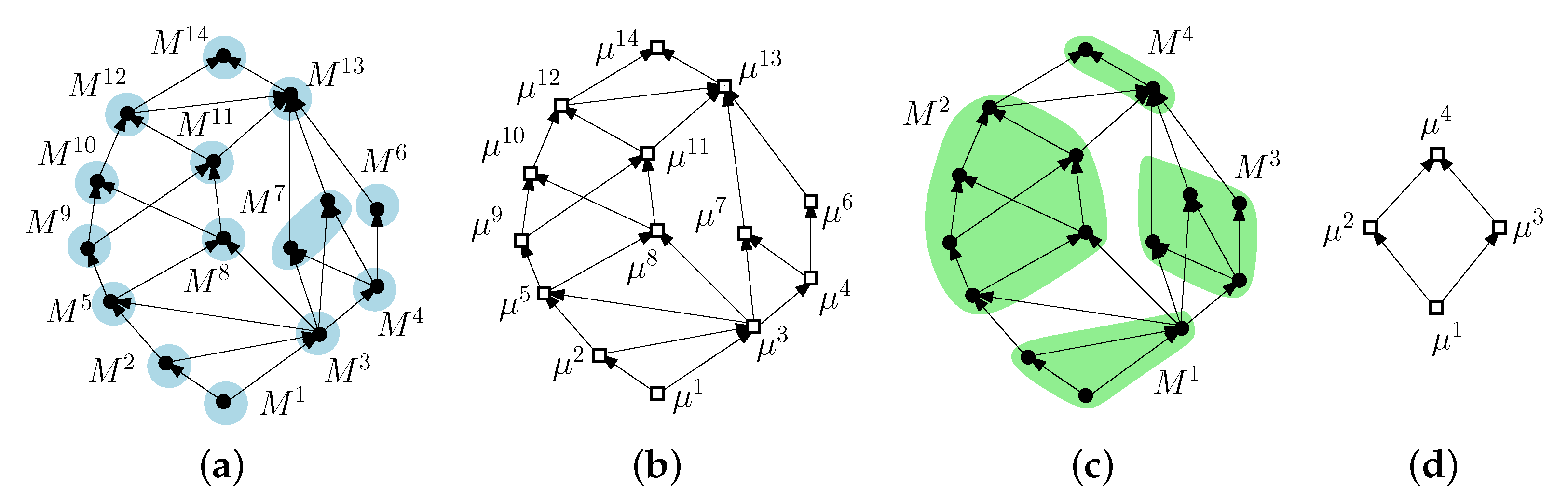
A module M of G is a non-empty subset of V such that either or, for any two vertices and any vertex : if, and only if ; if, and only if . The congruence partition of V is a partition of V into modules. The quotient graph is the graph obtained from G by merging the nodes of each module of . For a given module , we denote by the vertex representing M in . Figure 2a shows an -graph G and a congruence partition of it. Figure 2b shows the quotient graph .
In this paper, we use the concept of transitive module, transitive congruence partition, and transitive quotient graph of G, defined as a module, a congruence partition, and a quotient graph of the transitive closure graph of G. This concept is also used in [17], but there they simply call “module” a transitive module.
Formally, a transitive module of G is a non-empty subset of V such that either or, for any two vertices and any vertex : there is a path connecting to u if, and only if there is a path connecting to u; there is a path connecting u to if, and only if there is a path connecting u to . A transitive congruence partition of G is a partition of G into transitive modules. The transitive quotient graph is the graph obtained from G by merging the nodes of each transitive module of . For a given module , we denote by the vertex representing in .
Notice that every module of G is also a transitive module of G. Hence, the concepts of transitive module, transitive congruence partition, and transitive quotient graphs are a generalization of the concept of module, congruence partition, and quotient graph. For the rest of the paper, since we are going to talk only about transitive modules, transitive congruence partition, and transitive quotient graph, we will omit the symbol “” in the notation in order to simplify our presentation. Figure 2c shows the -graph G depicted in Figure 2a and a transitive congruence partition of G that is not a congruence partition. Figure 2d shows the transitive quotient graph .
The modular decomposition of G is a tree describing a decomposition of G based into modules of G. The root of the tree is the module , containing all the vertices of G, and the leaves of the tree are the singleton modules, where every singleton contains a vertex of G. The children of every non-leaf node M of the tree are the module of G contained in M and that are not contained in any other module contained in M.
The modular decomposition can be computed in time and it requires time to obtain a congruence partition and the correspondent quotient graph of G from a modular decomposition of G. For further details about modular decomposition see [18]. Computing a transitive congruence partition of G requires time, since we can obtain it by computing a congruence partition of the transitive closure graph of G.
Let be a transitive modular decomposition of G and let , where is the subset of edges of E that are incident to two vertices of . The congruence dimension of G given is the value . Since each is a subgraph of G and is obtained from G, one might consider that . In [19] it is proved that is an upper bound to .
Lemma 5.
For every -graph G and any transitive congruence partition of G, the following relation holds: [19].
For example, refer to Figure 2c, that depicts a graph G and its transitive congruence partition . We have that , , , and are upward planar and that has width equal to 2. Hence, by Lemma 1 and Inequality (2) of Lemma 2, for every and . Hence, and, by Lemma 5, . Since G does not contain a Hamiltonian path, . It follows that . Figure 4b shows a two-dimensional dominance drawing of G.
In Section 3.1 we show an algorithm to compute dominance drawings with the bound stated in Lemma 5. More formally, we describe an algorithm to compute a dominance drawing of any -graph G having dimensions given the set of a q-dimensional dominance drawing of the graphs associated to a transitive congruence partition of G, where . In Section 3.2 we discuss the time complexity of the algorithm.
3.1. Algorithm 2 (Proof of Lemma 5)
Let be a transitive congruence partition of G. Assume that, for any two vertices u and v so that and , if there is a path connecting u to v in G, then . It is possible to compute a labeling so that the above propriety holds by: Computing a topological sorting T of the vertices of the -graph (which is the quotient graph); setting i equal to the topological number of , , for any transitive module . Note that the two transitive congruence partitions depicted in Figure 2a,c (where the one of (a) is also a congruence partition) have a labeling with this property.
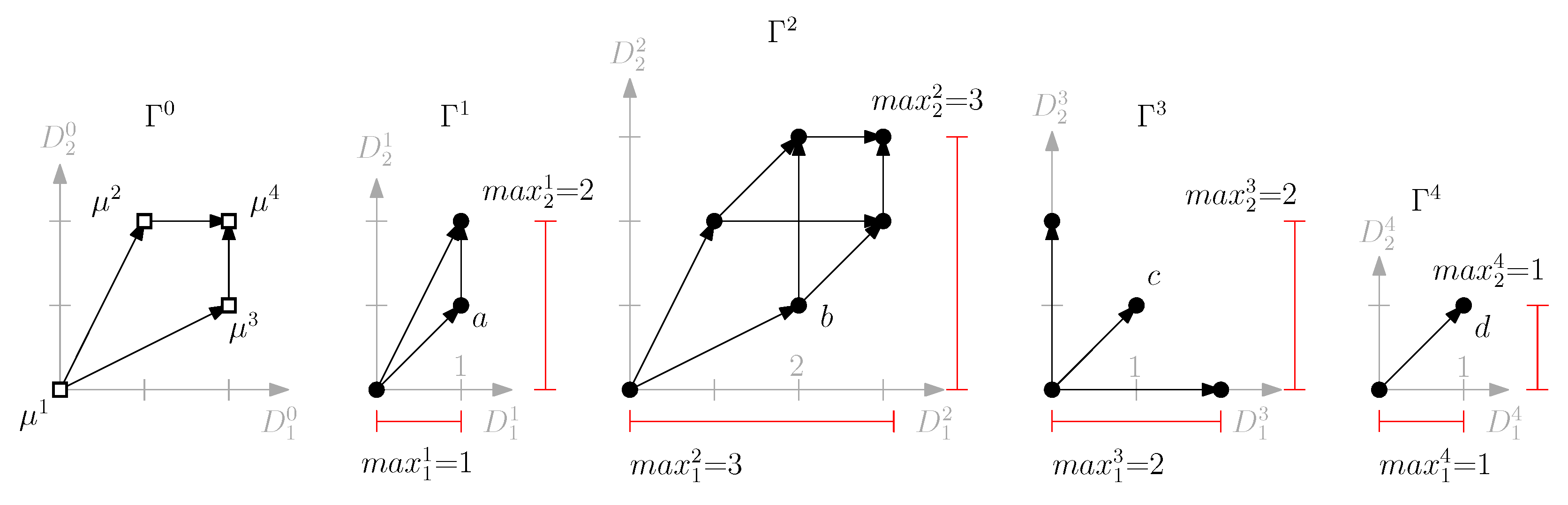
We denote graph by . Let be an ordered set of q-dimensional dominance drawings so that, for every , is a q-dimensional dominance drawing of . We prove that given , it is possible to obtain a q-dimensional dominance drawing of G. Then, since for every by definition of congruence dimension, the proof of Lemma 5 is a direct consequence of the fact that it is possible to set . See, for example, Figure 3 that depicts the drawings for the graph depicted in Figure 2c with transitive congruence partition . The transitive quotient graph is depicted in Figure 2d.
Notice that, given any dominance drawing of G with dimensions of a graph, it is possible to obtain a dominance drawing with q dimensions of the graph by adding to dimensions and by assigning to all the vertices of G the same position in the new dimensions. Hence, the assumption that all the drawings in the set have the same number of dimensions, q, is without loss of generality.
We now show Algorithm 3, which computes a q-dimensional dominance drawing of G. The algorithm consists of two steps, presented in detail in Section 3.1.1 and Section 3.1.2. We now give an overview of the algorithm.
| Algorithm 3 CP-Draw (Congruence Partition Draw). |
⋆ Input: An -graph and ⋆ Output: A h-dimensional drawing of G. Step 1: Compute a q-dimensional drawing of (different from ) having dimensions (see Figure 4a). We denote by skeleton drawing (see details in Section 3.1.1). Step 2: Compute a drawing (see Figure 4b) by using, for every vertex , the coordinates of in the skeleton drawing and of v in in order to set the coordinates of v in (see details in Section 3.1.2). |
In Section 3.1.2 we prove that is a q-dimensional dominance drawing.
3.1.1. Details of Step 1 of Algorithm 2: Preparing the Skeleton Drawing
We first introduce some notation. Let be the dimension in drawing and a number so that for every , where and . For every , we define the set to be the subset of so that, for any , if, and only if one of the two following cases holds: () ; () and (i.e., is not reachable from according to the labeling defined at the beginning of the section). Notice that the two cases never hold for and that, consequently, . Let .
Refer to Figure 3 for an example of the notation , , and defined above. The values , for , are computed as follow.
- i = 1:, since neither Case () nor Case () holds for , , and . Hence, .
- i = 2:, since Case () holds for and neither Case () nor Case () holds for vertices and . Hence, .
- i = 3:, since Case () holds for and and neither Case () nor Case () holds for vertex . Hence, .
- i = 4:, since Case () holds for and and Case () holds for .Hence, .
Let be a q-dimensional drawing of having dimensions so that, for every and every , .
3.1.2. Details of Step 2 of Algorithm 2: Computing a Dominance Drawing of
We construct a q-dimensional drawing of G having dimensions as follows: For every vertex , where , and for every , we set .
Refer to Figure 4b that depicts the drawing given of Figure 3 and of Figure 4a. Consider dimension and vertices , , , and , also depicted in Figure 3. We have: ; ; ; ;
Figure 4.
(a) The skeleton drawing given , where drawings are depicted in Figure 3. (b) The correspondent drawing .
Figure 4.
(a) The skeleton drawing given , where drawings are depicted in Figure 3. (b) The correspondent drawing .

Notice that, since q can be equal to and since is a q-dimensional drawing of G, in order to prove Lemma 5 it is sufficient to show that drawing is a dominance drawing of G.
Let u and v be two vertices of G. We prove that there is a path connecting u to v if, and only if for every . Suppose and , where . We distinguish two cases. In the first case u and v belong to the same transitive module, that is, , and in the second case u and v belong to two different transitive modules, that is, .
In the first case, , since is a dominance drawing, we have that there is a path connecting u to v if, and only if for every . We also have that, for every , implies since and , where . Hence, there is a path connecting u to v if, and only if for every .
For the rest of the proof we consider the second case, that is, . Suppose that there is a path connecting u to v in G. We prove that for every . Observe that a path from u to v always implies a path from to in and, since is a dominance drawing of , we have the following relation:
Since there is a path from to then, according to the labeling of the transitive modules based on the topological ordering of introduced at the beginning of the section, we have . Relation (1) implies . By Relation (1) and we have that either Case () or Case () holds for and that . Hence, and consequently we have the following relation:
We have , since is by definition the maximum value of a coordinate in the dimension of drawing . By Relation (1) . By Relation (2) . Hence, . This implies that for every .
Suppose that for every . We prove that there is a path connecting u to v in G. We first prove the following claim.
Claim 1.
Let u and v be two vertices of G so that and . For any , if then .
Proof.
We have and . Hence, since , . Therefore, we have the following relation:
Suppose for a contradiction that . It implies . Additionally, it implies that Case () holds for and that . We have and consequently . It follows that:
Substituting in Relation (3) the result of Relation (4) we have Since , we have It follows that and, consequently, , which is a contradiction. It follows that . □
In order to conclude the proof of Lemma 5 we present the following argument. Since by hypothesis for every , by Lemma 1 for every . Since is a dominance drawing of by hypothesis and since for every , then there is a path connecting to in . Therefore, there is a path connecting any vertex of to any vertex of in G and, consequently, there is a path connecting u to v in G.
We proved that for any two vertices u and v of G we have that there is a path from u to v if, and only if for every . Hence, drawing is a q-dimensional dominance drawing of G. Since q is equal to .
3.2. Complexity Analysis
In the previous section we showed an algorithm to compute dominance drawing with the bound stated in Lemma 5. In this section we do a worst-case analysis of the time complexity required to compute the dominance drawing .
Denote by the time required to compute the transitive congruence partition of G and by the time required to compute the set of q-dimensional dominance drawings of graphs . Given , it is possible to compute the values and for every and every in overall time. Hence, the time required to compute is . Therefore, we have the following theorem:
Theorem 3.
Let G be any -graph and let be a transitive congruence partition. Let be the time to compute and be the time to compute the set of q-dimensional dominance drawings , where . Then, it is possible to compute a q-dimensional dominance drawing of G in time.
We now give examples of possible values of and . Recall that computing a congruence partition requires [18]. It is possible to compute a transitive congruence partition in by computing a congruence partition of the transitive closure graph of G. Hence, it is possible to have . Let be the width of for every . If we compute the drawings by using the algorithm described in Section 2, then, by Theorem 2, , where . Notice that and that, in this case, by the theorem, it is possible to compute an -dimensional dominance drawing. We have if all the graphs are upward planar [2]. We summarize the result for the special cases described in the above paragraph with the following corollary.
Corollary 1.
It is possible to compute a -dimensional dominance drawing of G in time, where .
3.3. A Comparison between the Algorithms
In this section we show that by using the algorithm described in this section it is possible to compute dominance drawing with less dimensions with respect to the ones that we can compute by using the algorithm in Section 2.
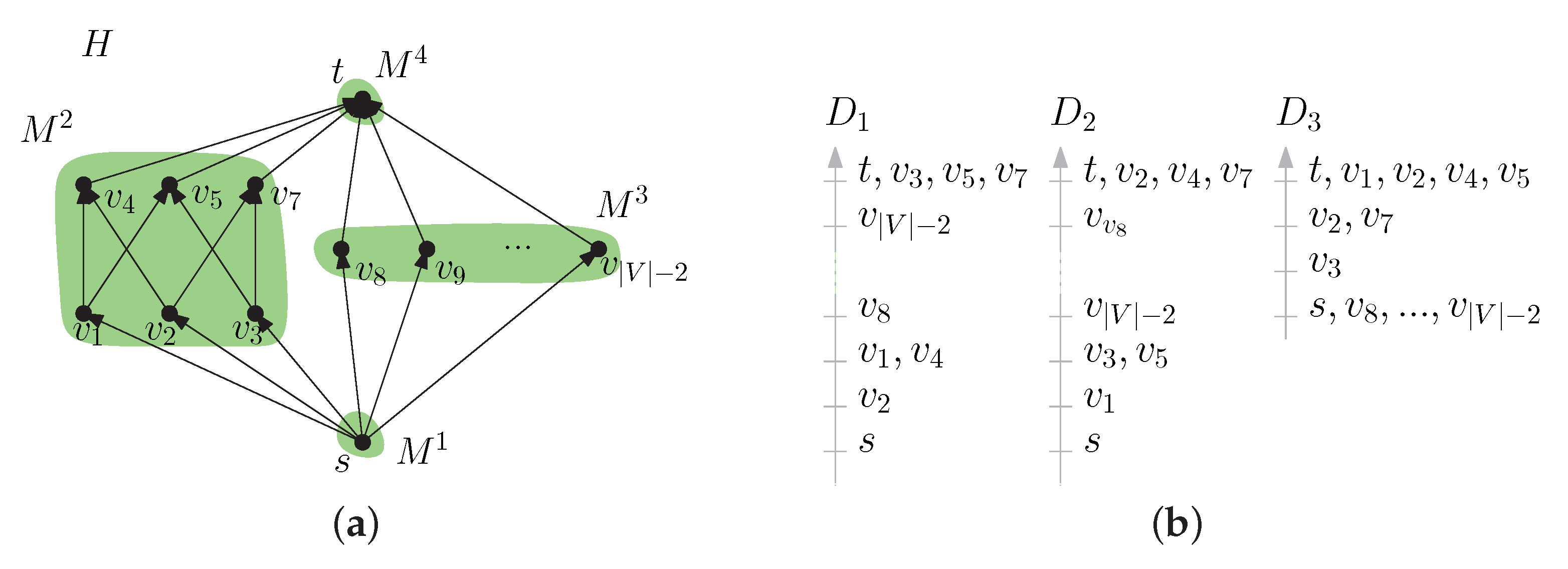
Let H be an -graph with n vertices, source s, sink t, and having a transitive congruence partition , where: ; for , is a crown graph; is a set containing incomparable vertices. See Figure 5a, where .
Let f be the width of H. We have , since is a set containing incomparable vertices. Additionally, it is well known that the crown graph has dominance dimension higher than 2, see for example [9]. Therefore, for every and . According to Lemmas 1 and 2 the best-known upper bound for is .
The graphs , where , are upward planar. Hence, for every by Lemma 1. For every , the width of is 3 and, since , we have by Inequality (2) of Lemma 2. Hence, . By Lemma 5 and by we have , which is optimum.
It is possible to construct the three-dimensional dominance drawings of , for , by Lemma 1 and by adding a third dimension as described at the beginning of Section 3.1. For every , it is possible to construct the three-dimensional dominance drawing of by Theorem 2. Hence, given , it is possible to construct and the three-dimensional dominance drawing of H as described in the proof of Lemma 5. Figure 5b depicts, for every , the values , , associated to the dimensions , , and of the drawing , where graph H is depicted in Figure 5a.
4. A Discussion on Weak Dominance Drawings
In this section we discuss the concept of weak dominance drawings, which is a generalization of the concept of dominance drawing. We point out the reason why it was introduced and we show two recent papers showing that this concept can be very useful in practice.
Given two vertices u and v of a DAG G, checking if there exists a directed path from u to v is denoted by reachability query. The problem of answering efficiently to reachability queries is widely studied in the literature. See, for example [10,17,20]. See also the following two very recent papers [21,22] and see [23] for a survey.
Dominance Drawing is a concept that can be very useful for answering reachability queries, that is, checking the existence of a path connecting two vertices in graph databases.Recall that given a dominance drawing of a DAG G having k dimensions, it is possible to answer to a reachability query very efficiently in time by using space. By using some clever strategy, as for the algorithm described in Section 2, the time can also be , that is, independent of the number of dimensions.
Computing dominance drawings of DAGs having a low number of dimensions would be important in practice. Unfortunately, most of the existing algorithms obtaining dominance drawings require the input DAG to have specific properties, that is, to be planar, as stated in Lemma 1. The algorithms that we presented so far avoid this problem, since no restriction on the input graph is given. On the other hand, the computational time required to compute dominance drawings is still not linear. For example, for the algorithm described in Section 2 computes f-dimensional dominance drawings in time, where n and f are the number of nodes and the width of G, respectively. When the number of vertices is very large, computing such drawings can be prohibitively expensive. By using heuristics for the computation of (sub-optimal) chain covers we can make the algorithms faster. Another possibility is to relax the concept of dominance. As we are going to observe in the rest of this section, this direction was studied by several authors.
The concept of weak dominance, a relaxed version of dominance, was introduced in [9]. The “if and only if” of dominance becomes an “if” in weak dominance. Namely, in a weak dominance drawing of a DAG , two vertices are incomparable in G if there exists two dimensions D and such that and . Unfortunately, u and v can be incomparable while for any dimension D of . In this case there is a falsely implied path (fip) between u and v. Clearly, any DAG G admits a k-dimensional weak dominance drawing for any integer k. For example, any topological order of the vertices of G is a one-dimensional weak dominance drawing of G. In [24] it is studied an interesting variation of the weak dominance drawing problem.
Given a weak dominance drawing , if there are two dimensions D and of such that and , then u and v are incomparable. This computation requires time. Otherwise, more expensive computations are needed to check weather there is a path connecting u and v. For example, a Breadth First Search (BFS) would take time per search. Minimizing the number of fips minimizes the number of BFS operations required by the drawing and, consequently, the average time required for a reachability query. Notice that minimizing the number of fips is NP-hard [9,25]. The weak dominance drawings were recently used to construct compact representations of the reachability information in databases [4,10].
Interesting experiments on algorithms computing weak dominance drawings are presented in [4,10]. They show that by using weak dominance drawings, it is possible to answer reachability queries more efficiently with respect to previous results. In [10] they use weak dominance drawing with more than two dimensions in order to have less fips and they show that even by using few dimensions, that is, by using almost linear space, it is possible to improve the results significantly. Extending [10], Lionakis et al. [11] show that, for the same families of graphs considered in [10] and by using a number of dimensions similar to the ones used in [10], it is possible to compute dominance drawings (i.e., 0 fips).
The technique used in [11] is similar to the one described in Section 2 of this paper. The computational time required to compute dominance drawings in [11] is still higher than the one to compute weak dominance drawings [10]. However, these results suggest that a possible direction for this line of research is to actually use directly dominance drawings instead of weak dominance drawings. In fact, in Section 3 we presented algorithms that compute dominance drawings with a reduced number of dimensions with respect to the ones presented in Section 2, and consequently in [10,11].
5. Conclusions and Open Problems
In this paper, we reviewed some mathematical results on dominance drawings of DAGs and their dimension, and presented an efficient algorithm that, for every -graph G with width f, constructs an f-dimensional dominance drawing. As far as we know, these are the most efficient algorithms to construct dominance drawings for any input DAG with a number of dimension that is described by the theoretical bounds.
We used the concept of congruence dimension of G given a transitive congruence partition of G, and we presented an efficient algorithm to compute a dominance drawing of G in dimensions. The congruence dimension of G is a better upper bound of the dominance dimension of G. Indeed, we showed that there exists a family of graphs so that for every graph H of the family the best-known upper bound of , according to Hiraguchi’s Theorem (Inequality (1) of Lemma 2), was and we proved that, according to Lemma 5, .
Notice that the number of dimensions used by a dominance drawing may be large, and the algorithm to compute it requires time. Therefore, it may be prohibitive for very large data sets as the ones used recently by the database community. There are three ways to approach these problems from theoretical and practical points of view:
- Use a relaxed version of dominance drawing called weak dominance drawing, see [9]. The existence of fips cannot be excluded since the number of dimensions in a weak dominance drawing is typically significantly less than . Hence, computing such drawings with few fips is central to any approach involving weak dominance drawings. Recall that minimizing the number of fips is NP-hard [9,25]. Additionally, using more dimensions in a weak dominance drawing reduces the number of fips. It would be interesting to experimentally study this tradeoff.
- Explore heuristics in order to compute dominance drawings of DAGs in “almost linear time”, even if they need a higher number of dimensions. This would be another interesting research direction given the high complexity required by current algorithms.
- Finally, an interesting theoretical open problem is to find algorithms that construct dominance drawings of similar quality as the ones computed by the current algorithms (that require time) but in less time, or prove a non-trivial lower bound for this construction.
Author Contributions
G.O. and I.G.T. contributed equally to this work. All authors have read and agreed to the published version of the manuscript.
Funding
The research of I.G.T. was supported in part by Tom Sawyer Software, Inc., Berkeley, CA, U.S.A.
Data Availability Statement
Data sharing is not applicable to this article.
Conflicts of Interest
The authors declare no conflict of interest.
References
- ElGindy, H.A.; Houle, M.E.; Lenhart, W.; Miller, M.; Rappaport, D.; Whitesides, S. Dominance Drawings of Bipartite Graphs. In Proceedings of the 5th Canadian Conference on Computational Geometry, Waterloo, ON, Canada, 8–10 August 1993; University of Waterloo: Waterloo, ON, Canada, 1993; pp. 187–191. [Google Scholar]
- Di Battista, G.; Tamassia, R.; Tollis, I.G. Area Requirement and Symmetry Display of Planar Upward Drawings. Discret. Comput. Geom. 1992, 7, 381–401. [Google Scholar] [CrossRef]
- Six, J.M.; Tollis, I.G. Automated Visualization of Process Diagrams. In Graph Drawing; Mutzel, P., Jünger, M., Leipert, S., Eds.; Springer: Berlin/Heidelberg, Germany, 2002; pp. 45–59. [Google Scholar]
- Veloso, R.R.; Cerf, L.; Meira, W., Jr.; Zaki, M.J. Reachability Queries in Very Large Graphs: A Fast Refined Online Search Approach. In Proceedings of the 17th International Conference on Extending Database Technology (EDBT 2014), Athens, Greece, 24–28 March 2014; pp. 511–522. [Google Scholar]
- Yannakakis, M. The complexity of the partial order dimension problem. SIAM J. Algebr. Discret. Methods 1982, 3, 303–322. [Google Scholar] [CrossRef]
- Battista, G.D.; Eades, P.; Tamassia, R.; Tollis, I.G. Graph Drawing: Algorithms for the Visualization of Graphs; Prentice Hall: Hoboken, NJ, USA, 1998; pp. 112–127. [Google Scholar]
- Dushnik, B.; Miller, E.W. Partially ordered sets. Am. J. Math. 1941, 63, 600–610. [Google Scholar] [CrossRef] [Green Version]
- McConnell, R.M.; Spinrad, J.P. Linear-Time Transitive Orientation. In Proceedings of the Eighth Annual ACM-SIAM Symposium on Discrete Algorithms, New Orleans, LA, USA, 5–7 January 1997; Saks, M.E., Ed.; ACM/SIAM: Philadelphia, PA, USA, 1997; pp. 19–25. [Google Scholar]
- Kornaropoulos, E.M.; Tollis, I.G. Weak Dominance Drawings for Directed Acyclic Graphs. In Proceedings of the Graph Drawing—20th International Symposium, GD 2012, Redmond, WA, USA, 19–21 September 2012; pp. 559–560, Revised Selected Papers. [Google Scholar] [CrossRef] [Green Version]
- Li, L.; Hua, W.; Zhou, X. HD-GDD: High dimensional graph dominance drawing approach for reachability query. World Wide Web 2017, 20, 677–696. [Google Scholar] [CrossRef]
- Lionakis, P.; Ortali, G.; Tollis, I.G. Constant-Time Reachability in DAGs Using Multidimensional Dominance Drawings. SN Comput. Sci. 2021, 2, 320. [Google Scholar] [CrossRef]
- Jagadish, H.V. A Compression Technique to Materialize Transitive Closure. ACM Trans. Database Syst. 1990, 15, 558–598. [Google Scholar] [CrossRef]
- Bogart, K.P. Maximal dimensional partially ordered sets I. Hiraguchi’s theorem. Discret. Math. 1973, 5, 21–31. [Google Scholar] [CrossRef] [Green Version]
- Hiraguchi, T. On the dimension of partially ordered sets. Sci. Rep. Kanazawa Univ. 1951, 1, 77–94. [Google Scholar]
- Dilworth, R.P. A decomposition theorem for partially ordered sets. Ann. Math. 1950, 52, 161–166. [Google Scholar] [CrossRef]
- Chen, Y.; Chen, Y. On the DAG Decomposition. Br. J. Math. Comput. Sci. 2015, 10, 1–27. [Google Scholar] [CrossRef] [PubMed]
- Anirban, S.; Wang, J.; Islam, M.S. Modular Decomposition-Based Graph Compression for Fast Reachability Detection. Data Sci. Eng. 2019, 4, 193–207. [Google Scholar] [CrossRef] [Green Version]
- McConnell, R.M.; Spinrad, J.P. Modular decomposition and transitive orientation. Discret. Math. 1999, 201, 189–241. [Google Scholar] [CrossRef] [Green Version]
- Möhring, R. Computationally Tractable Classes of Ordered Sets. In Algorithms and Order; Rival, I., Ed.; NATO ASI Series (Series C: Mathematical and Physical Sciences); Springer: Dordrecht, The Netherlands, 1989; Volume 255. [Google Scholar] [CrossRef]
- Su, J.; Zhu, Q.; Wei, H.; Yu, J.X. Reachability Querying: Can It Be Even Faster? IEEE Trans. Knowl. Data Eng. 2017, 29, 683–697. [Google Scholar] [CrossRef]
- Yang, L.; Chen, T.; Zhang, J.; Long, J.; Hu, Z.; Sheng, V.S. Fruited-Forest: A Reachability Querying Method Based on Spanning Tree Modelling of Reduced DAG. In Web and Big Data, Proceedings of the 4th International Joint Conference, APWeb-WAIM 2020, Tianjin, China, 18–20 September 2020; Wang, X., Zhang, R., Lee, Y., Sun, L., Moon, Y., Eds.; Lecture Notes in Computer Science; Springer: Berlin/Heidelberg, Germany, 2020; Volume 12317, pp. 145–153. [Google Scholar] [CrossRef]
- Zhou, J.; Yu, J.X.; Li, N.; Wei, H.; Chen, Z.; Tang, X. Accelerating reachability query processing based on DAG reduction. VLDB J. 2018, 27, 271–296. [Google Scholar] [CrossRef]
- Yu, J.X.; Cheng, J. Graph Reachability Queries: A Survey. In Managing and Mining Graph Data; Springer: Boston, MA, USA, 2010. [Google Scholar]
- Ferreira da Silva, R.; Urrutia, S.; dos Santos, V.F. One-Sided Weak Dominance Drawing. Theor. Comput. Sci. 2019, 757, 36–43. [Google Scholar] [CrossRef]
- Kornaropoulos, E.M.; Tollis, I.G. Weak Dominance Drawings and Linear Extension Diameter. arXiv 2011, arXiv:1108.1439. [Google Scholar]
Figure 1.
(a) A chain cover of G, where: and . We have: ; ; ; ; ; ; ; . (b) The compressed transitive closure of G given . (c) The drawing .
Figure 1.
(a) A chain cover of G, where: and . We have: ; ; ; ; ; ; ; . (b) The compressed transitive closure of G given . (c) The drawing .

Figure 2.
(a) An -graph G and congruence partition of it. (b) The quotient graph . (c) Graph G depicted in (a) and a transitive congruence partition of it that is not a congruence partition. (d) The transitive quotient graph .
Figure 2.
(a) An -graph G and congruence partition of it. (b) The quotient graph . (c) Graph G depicted in (a) and a transitive congruence partition of it that is not a congruence partition. (d) The transitive quotient graph .

Figure 3.
The drawings for the graph G depicted in Figure 2c with transitive congruence partition . The transitive quotient graph is depicted in Figure 2d.

Figure 5.
Illustration of the example described in Section 3.3.
Figure 5.
Illustration of the example described in Section 3.3.

Publisher’s Note: MDPI stays neutral with regard to jurisdictional claims in published maps and institutional affiliations. |
© 2021 by the authors. Licensee MDPI, Basel, Switzerland. This article is an open access article distributed under the terms and conditions of the Creative Commons Attribution (CC BY) license (https://creativecommons.org/licenses/by/4.0/).
Share and Cite
MDPI and ACS Style
Ortali, G.; Tollis, I.G. Multidimensional Dominance Drawings and Their Applications. Foundations 2021, 1, 271-285. https://0-doi-org.brum.beds.ac.uk/10.3390/foundations1020020
AMA Style
Ortali G, Tollis IG. Multidimensional Dominance Drawings and Their Applications. Foundations. 2021; 1(2):271-285. https://0-doi-org.brum.beds.ac.uk/10.3390/foundations1020020
Chicago/Turabian StyleOrtali, Giacomo, and Ioannis G. Tollis. 2021. "Multidimensional Dominance Drawings and Their Applications" Foundations 1, no. 2: 271-285. https://0-doi-org.brum.beds.ac.uk/10.3390/foundations1020020