Big Rip Scenario in Brans-Dicke Theory

Abstract

In this work, we present a Big Rip scenario within the framework of the generalized Brans-Dicke (GBD) theory. In the GBD theory, we consider an evolving BD parameter along with a self-interacting potential. An anisotropic background is considered to have a more general view of the cosmic expansion. The GBD theory with a cosmological constant is presented as an effective cosmic fluid within general relativity which favours a phantom field dominated phase. The model parameters are constrained so that the model provides reasonable estimates of the Hubble parameter and other recent observational aspects at the present epoch. The dynamical aspects of the BD parameter and the BD scalar field have been analysed. It is found that the present model witnesses a finite time doomsday at a time of $t_{BR}\simeq 16.14\mathrm{Gyr}$, and for this scenario, the model requires a large negative value of the Brans-Dicke parameter.

1. Introduction

Late-time cosmic acceleration is one of the most bizarre and unsolved problems in modern cosmology. In scalar field cosmological models, the late-time cosmic acceleration issue is predominantly attributed to an exotic dark energy (DE) form that corresponds to a cosmic fluid having low energy density, as well as negative pressure. This is usually understood through a quantity dubbed as the equation of state (EoS) parameter ${\omega }_D=\frac{p}{\rho }$, where p represents the DE pressure and $\rho$ symbolises the dark energy density. The dark energy with a negative pressure corresponds to a negative EoS parameter. Despite several attempts made by astronomers and cosmologists, the experimental determination of ${\omega }_D$ remains challenging. Its precise estimation at the present epoch along with the knowledge of its development over a long period may unravel the mystery of the dark energy whose nature and origin remains speculative so far. In the $\mathsf{\Lambda }$CDM model, the cosmological constant $\mathsf{\Lambda }$ with ${\omega }_D=1$ plays the role of dark energy. However, in canonical scalar field models, quintessence fields or phantom fields shoulder the burden for the late-time cosmic speed-up, while the EoS parameter for the quintessence field lies in the range $-\frac{2}{3}\le {\omega }_D\le -\frac{1}{3}$ [1,2,3], which for the phantom fields, becomes ${\omega }_D<-1$ [4]. However, the EoS parameter as constrained from recent observational data favours a phantom phase in the Universe with ${\omega }_D<-1$ [5], while constraints from the CMB data in the nine-year WMAP survey suggest that ${\omega }_D=-1.{073}_{-0.089}^{+0.090}$ [6], a combination of the CMB data with Supernova data, predicts ${\omega }_D=-1.084\pm 0.063$ [7]. Other constraints on the EoS parameter include ${\omega }_D=-1.{035}_{-0.059}^{+0.055}$ from Supernova cosmology project [8], ${\omega }_D=-1.03\pm 0.03$ from recent Planck 2018 results [9] and from Pantheon data ${\omega }_D=-1.006\pm 0.04$ [10]. In phantom dark energy models, the energy conditions are usually violated, and the Universe may witness a blowing-up of the curvature of space-time at a finite time, leading to the dissolution of the whole material Universe into pieces. This picture of the finite future of the Universe, dubbed as the Big Rip singularity, concerns the recent cosmological research [11,12]. The finite-time future singularity leads to inconsistencies which led to different proposals in recent times, including the quantum effects to delay singularity, possible gravity modification, or the coupling of dark energy and dark matter [13,14].

In recent times, because of the concern regarding the ultimate fate of the Universe for phantom accreted dark energy with ${\omega }_D<-1$, a number of cosmological models have been used to investigate the Rip cosmologies based on the general relativity (GR) and modified gravity. Darbowski et al. studied the Big Rip singularity and the ultimate cosmic fate [15,16], and Granda and Loaiza showed the occurrence of Big Rip for kinetic and Gauss-Bonnet coupling [17]. The classical and quantum fate of the Big Rip cosmology has been studied by Vasilev et al. [18]. Within the framework of $f\left(T\right)$ gravity, Hanafy and Saridakis presented a cosmological model where the Universe may last forever in a Pseudo Rip scenario [19]. Recently, Ray et al. studied the Big Rip and some Pseudo Rip cosmological models in the context of an extended gravity theory [20], and Pati et al. investigated the possible occurrence of Rip scenarios in an extended symmetric teleparallel theory [21]. Big Rip singularity is a unique singularity that possibly occurs in a phantom scenario violating the Null Energy Condition. The occurrence of Big Rip singularity, for which the energy density and the scale factor of the Universe diverge, dissolutes the bound system and ultimately leads to the tearing up of the Universe in finite time. Such a scenario has become a major concern for cosmologists. As such, the present study is aimed at investigating the possibility of the occurrence of a Big Rip scenario within the framework of the generalised Brans-Dicke (GBD) theory. The GBD theory incorporates a self-interacting potential, as well as a dynamically varying Brans-Dicke (BD) parameter. Previously, Montenegro and Carneiro have investigated some cosmological models leading to Big Rip kinds of solutions within the Brans-Dicke theory in the presence of decaying vacuum density. In that work, they considered a time-independent negative BD parameter $\omega =-1$ [22]. They obtained cosmological solutions with a time-varying deceleration parameter which may lead to negative energy density. In general, the BD theory is a most popular modified gravity theory proposed as an alternative to GR, where the gravity is mediated by a scalar field. The BD theory has already been used emphatically in addressing many issues in cosmology and astrophysics including the explanation for the inflationary scenario [23]. Over a period of time, the BD theory has been well-studied through different tests, including the gravitational radiation from gravitational wave bursts [24,25,26,27].

The manuscript is presented as follows: In Section 2, the basic field equations for the GBD theory are estimated for an anisotropic LRS Bianchi I (LRSBI) metric. Additionally, the dynamics of the GBD theory when incorporating a cosmological constant is appraised. Section 3 is devoted to a Big Rip scenario through a scale factor that diverges at a specific time, and discusses the time evolution of the BD scalar field, BD parameter, and the self-interacting potential under the Big Rip scenario. Lastly, the conclusion is drawn, and a concise summary of the present investigation is given in Section 4. Throughout this work, we chose the natural unit system: $8\pi G_0=c=1$, where $G_0$ symbolises the Newtonian gravitational constant at the present epoch and c represents the speed of light in vacuum.

2. Basic Formalism

In a Jordan frame within the GBD theory with a self-interacting potential $V\left(\varphi \right)$ and a time-dependent BD parameter $\omega \left(\varphi \right)$, we have the action as [28,29]

$$S=\int d^{4}x\sqrt{-g}\left[\varphi R-\frac{\omega \left(\varphi \right)}{\varphi }{\varphi }^{,\mu }{\varphi }_{,\mu }-V\left(\varphi \right)+{\mathcal{L}}_m\right],$$

(1)

where R defines the curvature and ${\mathcal{L}}_m$ is the matter Lagrangian. The time-dependence aspect of the BD parameter emerges naturally in the Kaluza-Klein theory, string theory, or in the supergravity theory [30,31]. Different issues in cosmology have been investigated in recent times in the GBD framework with a time-dependent BD parameter [32,33,34,35,36]. Because of the GBD field equations may be obtained as [36,37]

$$\begin{array}{ccc}\hfill G_{\mu \nu }& =& \frac{T_{\mu \nu }}{\varphi }+{\displaystyle \frac{\omega \left(\varphi \right)}{{\varphi }^2}}\left[{\varphi }_{,\mu }{\varphi }_{,\nu }-\frac{1}{2}{g}_{\mu \nu }{\varphi }_{,\alpha }{\varphi }^{,\alpha }\right]+\frac{1}{\varphi }\left[{\varphi }_{,\mu ;\nu }-g_{\mu \nu }\square \varphi \right]-\frac{V\left(\varphi \right)}{2\varphi }{g}_{\mu \nu },\hfill \end{array}$$

(2)

$$\begin{array}{ccc}\hfill \square \varphi & =& {\displaystyle \frac{T}{2\omega \left(\varphi \right)+3}}-{\displaystyle \frac{2V\left(\varphi \right)-\varphi \frac{\partial V\left(\varphi \right)}{\partial \varphi }}{2\omega \left(\varphi \right)+3}}-{\displaystyle \frac{\frac{\partial \omega \left(\varphi \right)}{\partial \varphi }{\varphi }_{,\mu }{\varphi }^{,\mu }}{2\omega \left(\varphi \right)+3}},\hfill \end{array}$$

(3)

where □ represents the d’Alembert operator. A perfect fluid distribution with the energy-momentum tensor $T_{\mu \nu }=(\rho +p)u_{\mu }{u}_{\nu }+p{g}_{\mu \nu }$ is considered, so that the $T=g_{\mu \nu }{T}^{\mu \nu }$ is the trace. In order to model the universe, we consider an LRSBI universe [38]

$$d{s}^2=-d{t}^2+A^{2}d{x}^2+B^2(d{y}^2+d{z}^2).$$

(4)

Even though the present observable Universe is mostly isotropic and homogeneous and can be mostly described as an FRW metric, some of the observations obviously hint of a possible departure from isotropy [39,40,41,42]. The amount of cosmic anisotropy present may be very small, but we cannot simply rule out its possibility. Additionally, the LRSBI model resembles the flat FRW model, but allowed us to incorporate a small but finite anistropy in the model. The GBD field equations for the anisotropic model become [32,36]

$$\begin{array}{ccc}\hfill (2k+1){\xi }^2{H}^2& =& \frac{\rho }{\varphi }+\frac{\omega \left(\varphi \right)}{2}{\left(\frac{\dot{\varphi }}{\varphi }\right)}^2-3H\left(\frac{\dot{\varphi }}{\varphi }\right)+\frac{V\left(\varphi \right)}{2\varphi },\hfill \end{array}$$

(5)

$$\begin{array}{ccc}\hfill 2\xi \dot{H}+3{\xi }^2{H}^2& =& -\frac{p}{\rho }-\frac{\omega \left(\varphi \right)}{2}{\left(\frac{\dot{\varphi }}{\varphi }\right)}^2-2\xi H\left(\frac{\dot{\varphi }}{\varphi }\right)-{\displaystyle \frac{\ddot{\varphi }}{\varphi }}+{\displaystyle \frac{V\left(\varphi \right)}{2\varphi }},\hfill \end{array}$$

(6)

$$\begin{array}{ccc}\hfill (k+1)\xi \dot{H}+(k^2+k+1){\xi }^2{H}^2& =& -\frac{p}{\varphi }-\frac{\omega \left(\varphi \right)}{2}{\left(\frac{\dot{\varphi }}{\varphi }\right)}^2-(k+1)\xi H\left(\frac{\dot{\varphi }}{\varphi }\right)-{\displaystyle \frac{\ddot{\varphi }}{\varphi }}+{\displaystyle \frac{V\left(\varphi \right)}{2\varphi }}.\hfill \end{array}$$

(7)

In the above equations, $\xi =\frac{3}{k+2}$ is an anisotropic parameter where k is a positive constant that decides the relationship among the directional expansion rates: $\frac{\dot{A}}{A}=k\frac{\dot{B}}{B}$. One should note that the isotropic behaviour of the model may be obtained for $\xi =1$. $H=\frac{1}{3}\left(\frac{\dot{A}}{A}+2\frac{\dot{B}}{B}\right)=\frac{1}{\xi }\frac{\dot{B}}{B}$ is the Hubble parameter.

The BD scalar field satisfies the Klein-Gordon equation

$${\displaystyle \frac{\ddot{\varphi }}{\varphi }}+3H\frac{\dot{\varphi }}{\varphi }={\displaystyle \frac{\rho -3p}{2\omega \left(\varphi \right)+3}}-{\displaystyle \frac{\frac{\partial \omega \left(\varphi \right)}{\partial \varphi }{\dot{\varphi }}^2}{2\omega \left(\varphi \right)+3}}-{\displaystyle \frac{2V\left(\varphi \right)-\varphi \frac{\partial V\left(\varphi \right)}{\partial \varphi }}{2\omega \left(\varphi \right)+3}}.$$

(8)

The GBD theory may be recast as an effective GR picture by incorporating a cosmological constant $\mathsf{\Lambda }$. In such a case, the total energy density and the total pressure respectively become ${\rho }_T=\rho +\mathsf{\Lambda }$ and $p_T=p-\mathsf{\Lambda }$, and the GBD field equations reduce to

$$\begin{array}{ccc}\hfill (2k+1){\xi }^2{H}^2& =& {\rho }_T+{\rho }_{\varphi },\hfill \end{array}$$

(9)

$$\begin{array}{ccc}\hfill \left(\frac{k+3}{2}\right)\xi \dot{H}+\left(\frac{k^2+k+4}{2}\right){\xi }^2{H}^2& =& -\left(p_T+p_{\varphi }\right),\hfill \end{array}$$

(10)

where,

$$\begin{array}{ccc}\hfill {\rho }_{\varphi }& =& (2k+1){\xi }^2{H}^2\mathsf{\Delta }\varphi -3H\dot{\varphi }+\frac{\omega \left(\varphi \right)}{2}\left(\frac{{\dot{\varphi }}^2}{\varphi }\right),\hfill \end{array}$$

(11)

$$\begin{array}{ccc}\hfill p_{\varphi }& =& -\left(\frac{k^2+k+4}{2}\right){\xi }^2{H}^2\mathsf{\Delta }\varphi -\left(\frac{k+3}{2}\right)\xi \dot{H}\mathsf{\Delta }\varphi +\ddot{\varphi }+\left(\frac{k+3}{2}\right)\xi H\dot{\varphi }+\frac{\omega \left(\varphi \right)}{2}\left(\frac{{\dot{\varphi }}^2}{\varphi }\right),\hfill \end{array}$$

(12)

where $\mathsf{\Delta }\varphi =1-\varphi$, which ensures the reduction to GR behaviour for $\mathsf{\Delta }\varphi =0$. It is interesting to note here that the GBD theory provides an extra cosmic fluid which may shoulder the burden of late-time acceleration. The corresponding effective EoS parameter becomes

$${\omega }_{eff}=\frac{p_{\varphi }-\mathsf{\Lambda }}{{\rho }_{\varphi }+\mathsf{\Lambda }}=-1+\frac{-\left(\frac{k+3}{2}\right)\xi \dot{H}\mathsf{\Delta }\varphi +\left[(2k+1)-\left(\frac{k^2+k+4}{2}\right)\right]{\xi }^2{H}^2\mathsf{\Delta }\varphi +f(\varphi ,\dot{\varphi },\ddot{\varphi })}{\mathsf{\Lambda }+(2k+1){\xi }^2{H}^2\mathsf{\Delta }\varphi +g(\varphi ,\dot{\varphi })},$$

(13)

with $f(\varphi ,\dot{\varphi },\ddot{\varphi })=\ddot{\varphi }+\left[\left(\frac{k+3}{2}\right)\xi -3\right]H\dot{\varphi }+\omega \left(\varphi \right)\left(\frac{{\dot{\varphi }}^2}{\varphi }\right)$ and $g(\varphi ,\dot{\varphi })=-3H\dot{\varphi }+\frac{\omega \left(\varphi \right)}{2}\left(\frac{{\dot{\varphi }}^2}{\varphi }\right)$.

In the low redshift epoch, there can be small values of $\left|\mathsf{\Delta }\varphi \right|$, and consequently, $\mathsf{\Lambda }$ becomes the dominant term in the denominator of the second term in Equation (13). Additionally, in the numerator of Equation (13), the contribution of $f(\varphi ,\dot{\varphi },\ddot{\varphi })$ may be neglected compared to other terms. In the limit of $\left|\mathsf{\Delta }\varphi \right|\to 0$, the effective EoS may be expressed as

$${\omega }_{eff}\simeq -1-\frac{\mathsf{\Delta }\varphi }{\mathsf{\Lambda }}\left[-\left(\frac{k+3}{2}\right)\xi \dot{H}+\left[(2k+1)-\left(\frac{k^2+k+4}{2}\right)\right]{\xi }^2{H}^2\right],$$

(14)

which may be reduced to

$${\omega }_{eff}\simeq -1+2\frac{\mathsf{\Delta }\varphi }{\mathsf{\Lambda }}\xi \dot{H}.$$

(15)

for a small departure from cosmic anisotropy. The above equation tells us that we get a quintessence-like phase for $\mathsf{\Delta }\varphi >0$ and a phantom-dominated phase for $\mathsf{\Delta }\varphi <0$, at least in the low redshift epochs. In an earlier work, it has been shown from the reconstruction of the BD scalar field from observational $H\left(z\right)$ data that $\mathsf{\Delta }\varphi <0$. This shows phantom-like behaviour in the GBD theory [38].

3. A Big Rip Scenario

An explanation of the late-time cosmic speed-up issue with dark energy requires that the EoS parameter should be ${\omega }_D<-1/3$. The cosmological constant corresponds to ${\omega }_D=-1$. For dark energy, cosmological models favouring ${\omega }_D<-1$ are usually dominated with phantom energy for which the energy density goes up with time violating the dominant energy condition. The energy density in a phantom dominated dark energy model is proportional to the scale factor. As a consequence, the scale factor blows up at a finite time $t_{BR}-t_0\simeq \frac{2}{3|1+{\omega }_D|}\frac{1}{H_0\sqrt{1-{\mathsf{\Omega }}_m}}$, where $H_0$ represents the present value of the Hubble parameter and $\mathsf{\Omega }\simeq 0.3$ is the matter density parameter [43]. Such a scenario is termed as the Big Rip, whose occurrence dissolutes the bounded system [43,44,45]. The Big Rip scenario in Phantom models leads to a unique singularity in the Universe and can be associated with the fundamental quantum gravity formalism [46].

We consider a Big Rip scenario with the scale factor evolving as

$$a\left(t\right)\simeq {\left(t_{BR}-t\right)}^{\alpha },$$

(16)

where $t_{BR}$ is the epoch where the scale factor blows up. $\alpha$ is a constant parameter related to the EOS parameter as

$$\alpha =\frac{2}{3(1+{\omega }_D)}.$$

(17)

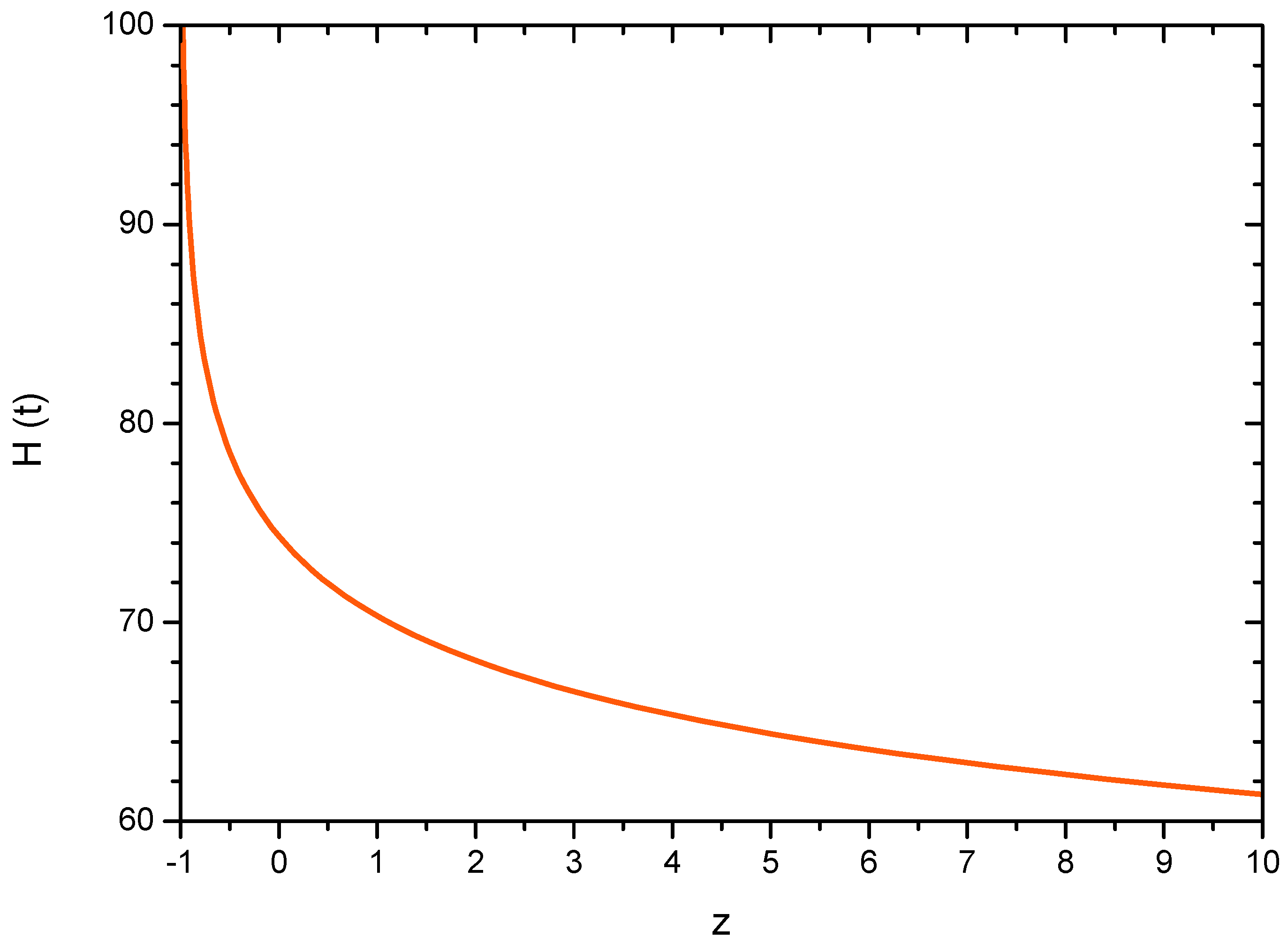
In a phantom field-dominated Universe, the EoS parameter is usually less than unity, that is, ${\omega }_D<-1$, which requires that the constant parameter $\alpha$ appearing in the scale factor should be negative, that is, $\alpha <0$. For the given Big Rip scenario, the Hubble parameter and the deceleration parameter (DP) are, respectively, $H\left(t\right)=-\frac{\alpha }{t_{BR}-t}$ and $q=-1-\frac{\dot{H}}{H^2}=-1+\frac{1}{\alpha }$. Additionally, we have $\dot{H}=-\frac{H^2}{\alpha }$ and $\ddot{H}=\frac{2}{{\alpha }^2}{H}^3$. One should note that, while the Hubble parameter contains two adjustable parameters, the deceleration parameter contains only one parameter, $\alpha$. The deceleration parameter in the present Big Rip scenario comes out to be a constant quantity which should be negative to provide an accelerating model. Because of this, we may constrain the parameter $\alpha$ from some recent observational constraint on the deceleration parameter. In a recent work, Camarena and Marra used the observational data from supernovae in a redshift range to constrain the DP as $q_0=-1.08\pm 0.29$ [47]. The central value of the deceleration parameter immediately fixes up the scale factor parameter as $\alpha =-12.49$. Consequently, the EoS parameter may be constrained as ${\omega }_D=-1.0533$. This value is in close agreement with some recent measurements, as mentioned earlier. Once $\alpha$ is fixed, the other parameter $t_{BR}$ may be obtained from the present value of the Hubble parameter. In Figure 1, we show the evolution of the Hubble parameter for the constrained value of $\alpha$ that predicts a finite-time future singularity. The Hubble parameter increases with the cosmic expansion and blows up at a finite future. Assuming $H_0=74.3$ km s⁻¹ Mpc⁻¹, the present model predicts a Big Rip occurring at a cosmic time $t_{BR}\simeq 16.14\mathrm{Gyr}$.

3.1. Brans-Dicke Scalar Field

Considering the Big Rip scenario, the evolutionary aspect of the Brans-Dicke scalar field may be studied within the framework of the GBD theory. Algebraic simplification of the field Equations (6) and (7) leads to the evolution equation for the BD scalar field as

$$-\frac{\dot{H}}{H}-3H=\frac{\dot{\varphi }}{\varphi }.$$

(18)

In terms of DP, we may express the evolution equation as

$$(q-2)H=\frac{\dot{\varphi }}{\varphi }.$$

(19)

In our model, we obtained the deceleration parameter to be a constant quantity, and consequently, the BD scalar field may be obtained by integrating Equation (19) as

$$\varphi =\frac{{\varphi }_0}{a_0^n}{a}^n,$$

(20)

where $n=q-2=\frac{1}{\alpha }-3$. $a_0$ and ${\varphi }_0$ are respectively the value of the scale factor and the BD scalar field at the present epoch. This relation clearly articulates a power-law behaviour of the BD scalar field with respect to the scale factor. It is worth mentioning here that the use of power-law functional behaviour of the scalar field is quite common in the literature. Since the deceleration parameter is a negative quantity in our model, the BD scalar field should decrease with the cosmic expansion.

The scale factor may be expressed as $a={\left(-\frac{\alpha }{H}\right)}^{\alpha }$, and consequently, the BD scalar field becomes

$$\frac{\varphi }{{\varphi }_0}={\left(\frac{H_0}{H}\right)}^{n\alpha },$$

(21)

which ultimately leads to

$$\frac{\ddot{\varphi }}{\varphi }=-3n{H}^2.$$

(22)

In terms of the redshift defined as $z=\frac{a_0}{a}-1$, the BD scalar field reduces to

$$\frac{\varphi }{{\varphi }_0}={(1+z)}^{-n}.$$

(23)

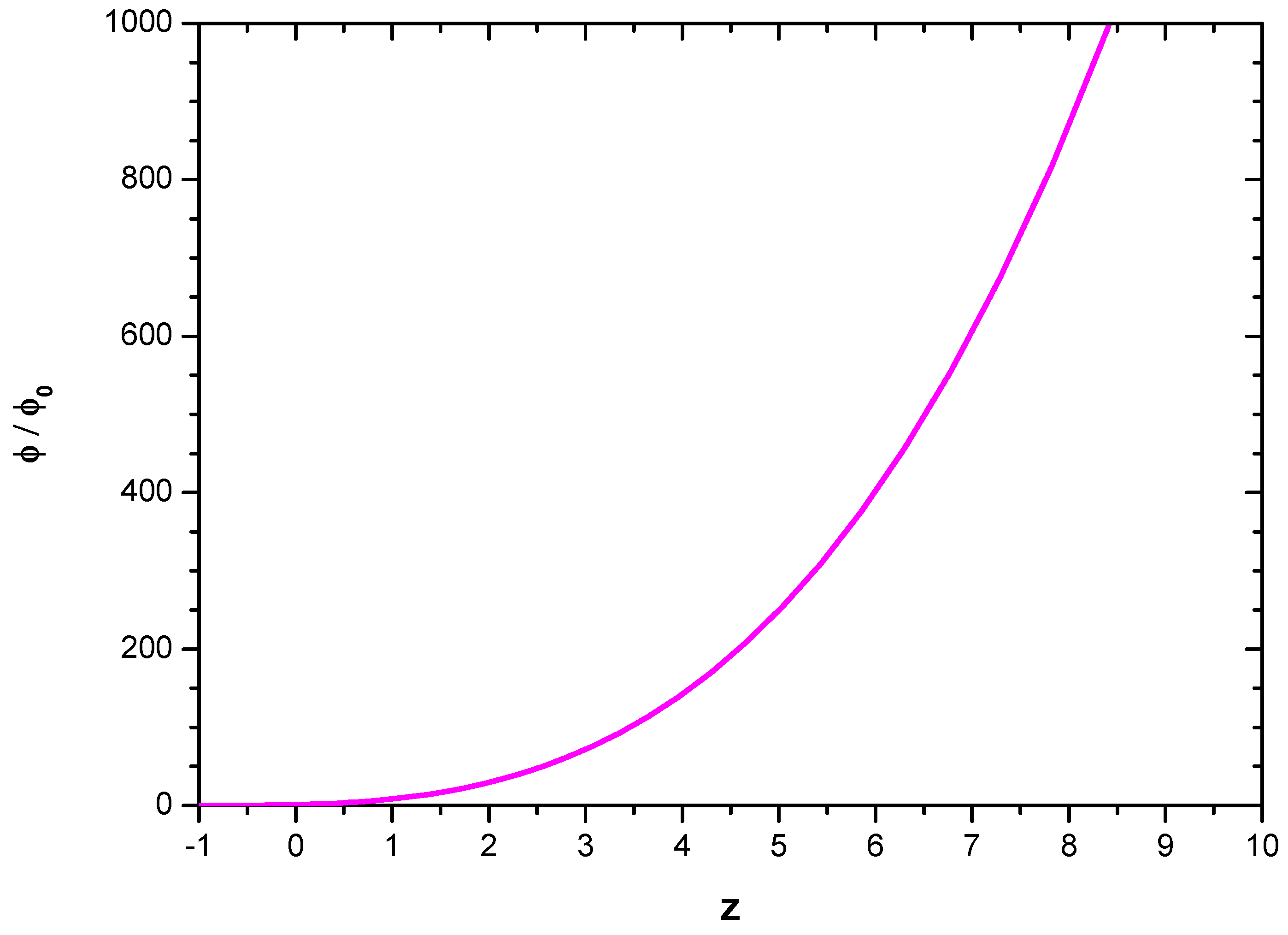
In Figure 2, the evolutionary aspect of the BD field is shown. The BD scalar field shows a decreasing trend from large positive values to vanishingly small values at late cosmic times. One should note from the figure that the BD scalar field behaves like ∼${\left(1+z\right)}^3$ in low redshift epochs.

3.2. Brans-Dicke Parameter

The BD parameter is a dynamical quantity in the GBD theory, and its behaviour depends on the dynamical behaviour of the BD scalar field. The BD parameter may be obtained from the GBD field Equations (5)–(7) as

$$\omega \left(\varphi \right)=\frac{1}{{\left(\frac{\dot{\varphi }}{\varphi }\right)}^2}\left[-{\displaystyle \frac{\rho +p}{\varphi }}-\frac{\ddot{\varphi }}{\varphi }+k\xi H\frac{\dot{\varphi }}{\varphi }-2\xi \dot{H}+2(k-1){\xi }^2{H}^2\right].$$

(24)

It should be mentioned here that, for a given Big Rip scenario as specified by a Hubble parameter H and a given cosmic anisotropy $\xi$, the dynamics of the BD scalar field is suitably obtained. Once the BD scalar field is obtained, the time-dependent aspect of the BD parameter now requires an equation of state $p={\omega }_D\rho$, a relationship between the pressure p and the energy density $\rho$. Replacing $\rho +p$ by $(1+{\omega }_D)\rho$ and using the fact that $\frac{\dot{\varphi }}{\varphi }=nH$ in Equation (24), we get

$$\omega \left(\varphi \right)=n^{-2}{H}^{-2}\left[-\left({\displaystyle \frac{1+{\omega }_D}{\varphi }}\right)\rho +\left((k\xi +3)n+2(k-1){\xi }^2\right)H^2\right].$$

(25)

For the given Big Rip scenario, the conservation equation for the cosmic fluid

$$\dot{\rho }+3H(\rho +p)=0$$

(26)

can be reduced to

$$\frac{\dot{\rho }}{\rho }=-\frac{2}{\alpha }H.$$

(27)

The energy density may be obtained from the integration of the conservation equation as

$$\rho ={\rho }_0{\left(\frac{H}{H_0}\right)}^2,$$

(28)

where ${\rho }_0$ is the present value of the energy density. Here, we used the fact that $\frac{a}{a_0}={\left(\frac{H_0}{H}\right)}^{\alpha }$. It is now straight-forward to obtain the pressure as

$$p=\left(\frac{2}{3\alpha }-1\right){\rho }_0{\left(\frac{H}{H_0}\right)}^2,$$

(29)

so that $p+\rho =\frac{2}{3\alpha }{\rho }_0{\left(\frac{H}{H_0}\right)}^2$. The Brans-Dicke parameter may now be expressed in terms of the Hubble parameter as

$$\omega (H,\xi ,\alpha )={\omega }_0(H_0,\xi ,\alpha )-\chi \left[{\left(\frac{H}{H_0}\right)}^{(n\alpha -2)}-1\right],$$

(30)

where $\chi =\frac{2{\rho }_0{H}_0^{\left(\right(3+n)\alpha -1)}}{3\alpha {\varphi }_0{n}^2}$ and ${\omega }_0(H_0,\xi ,\alpha )=\frac{k\xi +3}{n}+2(k-1){\left(\frac{\xi }{n}\right)}^2-\chi$ is the present value of the BD parameter.

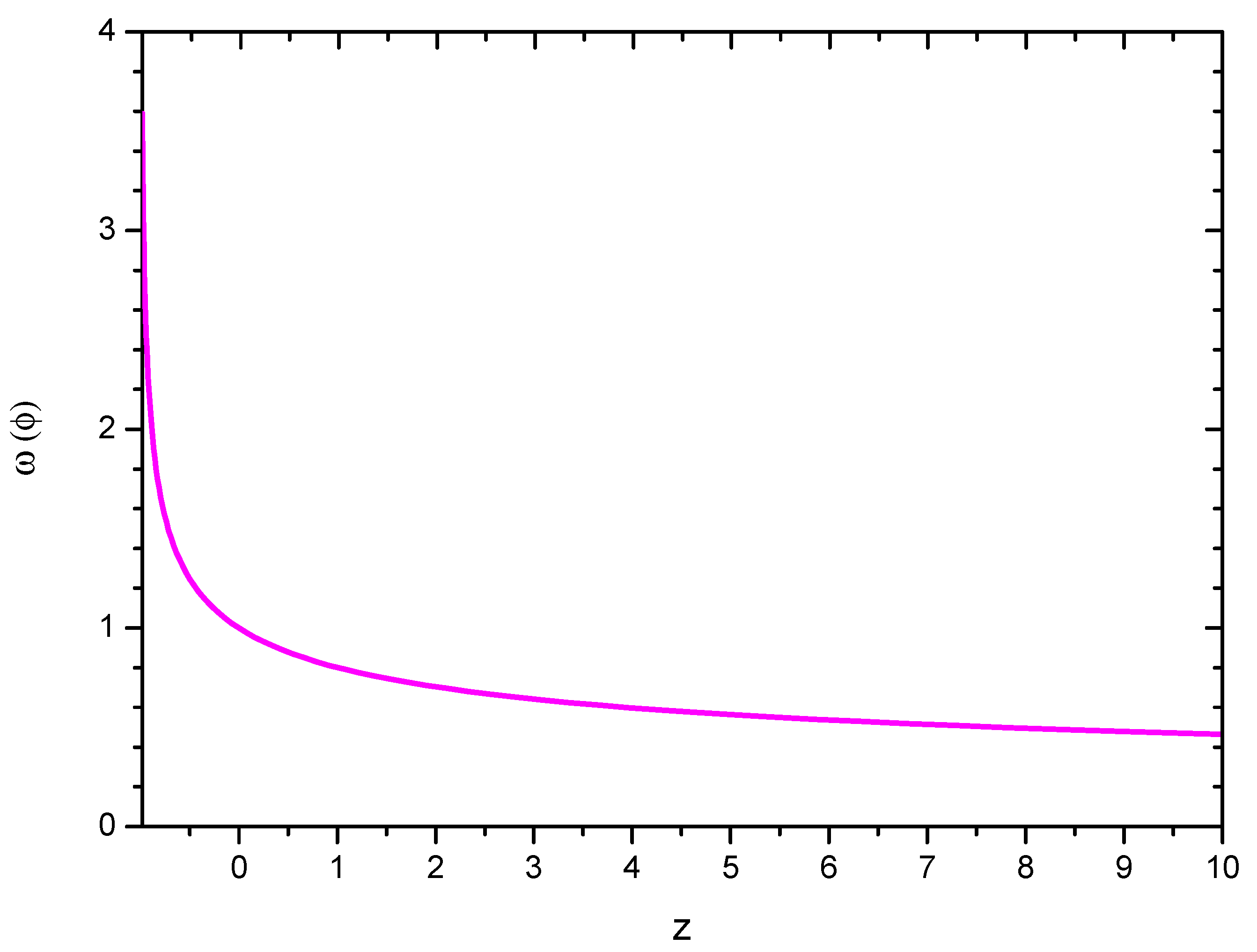
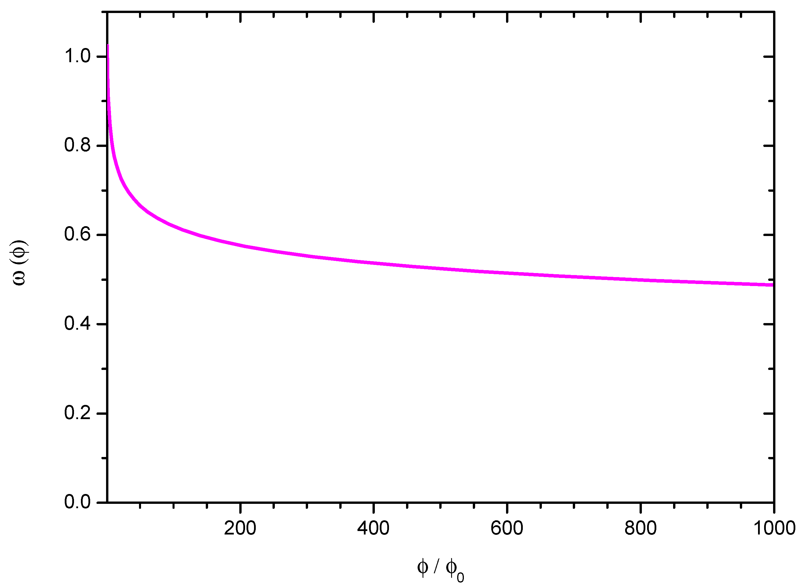
One may note that the anisotropy affects the Brans-Dicke parameter, but it does not participate in its evolution. Only the non-evolving part of the Brans-Dicke parameter is modified in the presence of cosmic anisotropy. In fact, as is evident from Equation (30), the cosmic anisotropy brings about a change in the required present value of the BD parameter. Similar results have already been observed in an earlier work [32], where it was shown that for a power-law expansion and an exponential expansion law of the scale factor, the cosmic anisotropy affects only that part of the BD parameter which does not evolve with time. The similarity between this Big Rip model and that of the power-law behaviour and the exponential expansion model is that the deceleration parameter is non-evolving. Because of this, we may infer that, for the time-independent deceleration parameter, the cosmic anisotropy will not contribute to the evolution of the Brans-Dicke parameter. However, for models with a time-dependent deceleration parameter, the cosmic anisotropy affects the BD parameter as a whole [36,38]. In Figure 3, the BD parameter (normalized to its value at the present epoch) is shown for a representative value of the cosmic anisotropy $\xi$. It is observed that the BD parameter increases with the cosmic expansion. Since the Hubble parameter blows up at a time $t\simeq t_{BR}$, the BD parameter also blows up at that epoch. In Figure 4, the evolutionary aspect of the BD parameter with respect to the BD scalar field is shown. With an increase in the BD scalar field, $\omega (H,\xi ,\alpha )$ decreases from a much higher value to low positive values. However, the decrement in $\omega (H,\xi ,\alpha )$ slows down for higher values of the scalar field. One may estimate the BD parameter at the present epoch within the purview of the present formalism to get a rip scenario at a finite future. In fact, for a finite time future singularity such as the one discussed in the present work within GBD theory, we require the BD parameter to be approximately $\omega (z=0)\simeq -3.6\times {10}^9$ at the present epoch.

3.3. Self-Interacting Potential

Within the GBD formalism, the time-dependence aspect of the self-interacting potential may be obtained as

$$V\left(\varphi \right)=2\varphi \left[\left\{(2k+1){\xi }^2+3n-\frac{\omega \left(\varphi \right)}{2}{n}^2\right\}{H}^2-\frac{\rho }{\varphi }\right].$$

(31)

In order to assess the effect of the cosmic anisotropy, we may express the self-interacting potential as

$$\frac{V\left(\varphi \right)}{2\varphi }=\left\{(2k+1){\xi }^2-\frac{{\omega }_0}{2}{n}^2\right\}{H}^2+\left[3n+\frac{\chi n^2}{2}\left({\left(\frac{H}{H_0}\right)}^{(n\alpha -2)}-1\right)\right]H^2-\frac{\rho }{\varphi }.$$

(32)

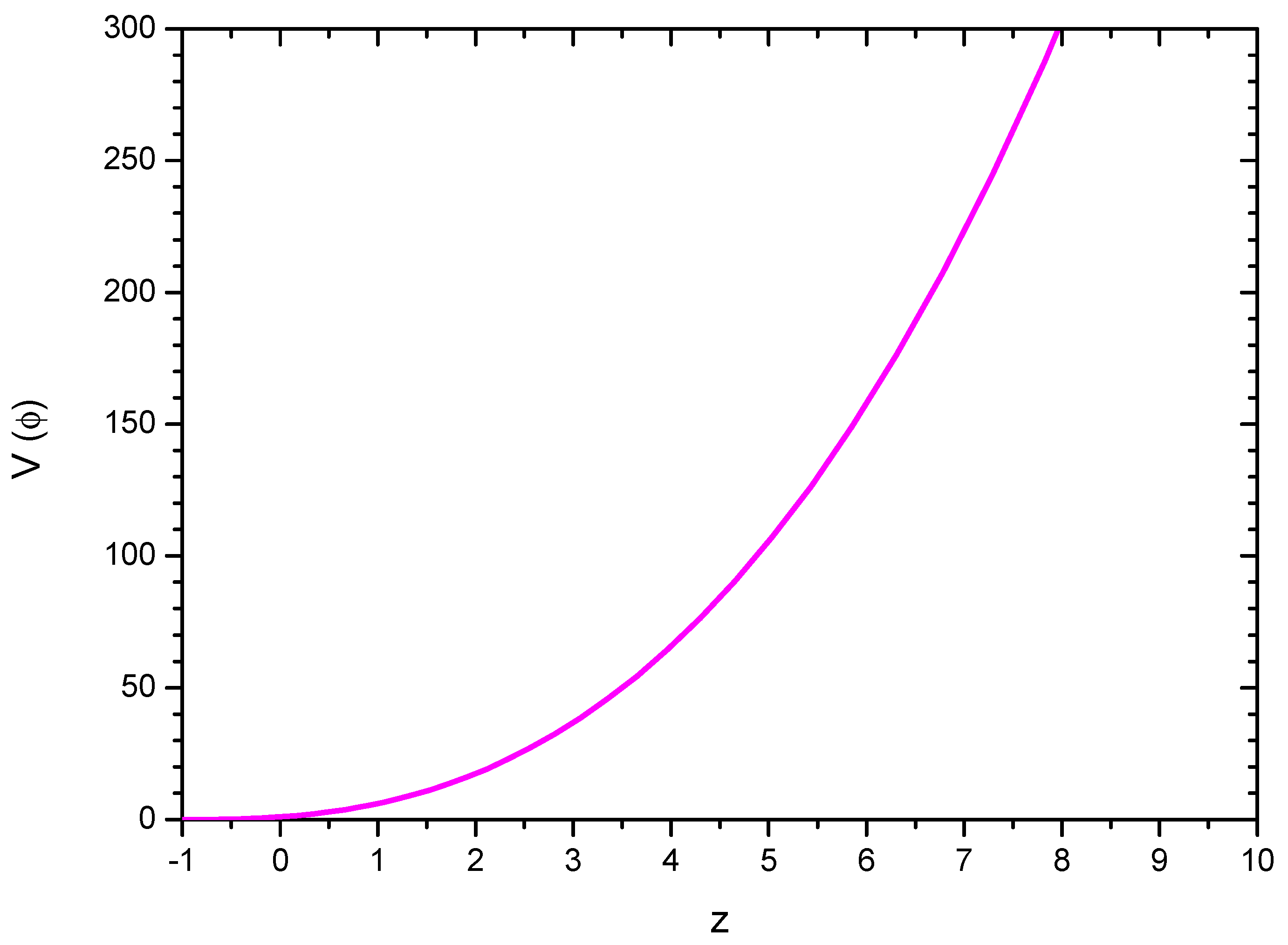
In the above Equation (32), the first term in the right-hand side bears the contribution of the cosmic anisotropy. In Figure 5, we show the evolutionary behaviour of the self-interacting potential for a given cosmic anisotropy. Since in the Big Rip scenario, we discussed in the present work a large negative value of ${\omega }_0=\omega (z=0)$ is being required, the effect of the cosmic anisotropy becomes negligibly small. However, in other scenarios such as a bouncing one, we may get a substantial effect of the cosmic anisotropy on the self-interacting potential [36]. Because of this, we chose a representative value $k=1.0001$ or a corresponding $\xi =0.999967$ to plot the figure. The value of the self-interacting potential in the figure is normalized to its present value. One should note that, with the growth of cosmic expansion, $V\left(\varphi \right)$ decreases from a higher value to small values at late times. This behaviour may be translated in terms of the scalar field to infer that the self-interacting potential shows an increasing trend with the BD scalar field.

4. Summary and Conclusions

In the present work, we studied a Big Rip scenario within the framework of a generalized Brans-Dicke theory. An LRSBI Universe is considered to incorporate directional anisotropy in the expansion rates. Such a model provides a more general approach compared to the FRW model. The generalized Brans-Dicke theory having a cosmological constant can be recast as a GR-like theory with cosmic fluid dominated by dark energy. The effective cosmological constant for such effective cosmic fluid dominated by dark energy may provide a quintessence-like or phantom-like behaviour depending on the nature of the scalar field. On the basis of the nature of the BD scalar field which has been reconstructed from the observational $H\left(z\right)$ data, we showed that the present model favours a phantom dark energy model. In Phantom models, the energy density and the scale factor may grow sharply within a finite time, leading to a Big Rip situation. We considered a Big Rip scale factor with an arbitrary parameter, that was fixed from a recent observational value of the deceleration parameter, which ultimately fixes the effective EoS parameter as ${\omega }_D=-1.05$ in close conformity with recent observational estimates. Additionally, the present model witnesses a Big Rip scenario at a time $t_{BR}\simeq 16.14\mathrm{Gyr}$. We studied the dynamical aspects of the scalar field, Brans-Dicke parameter, and the self-interacting potential. In conformity with other scalar field models, the BD scalar field shows a decreasing behaviour with cosmic time. The Brans-Dicke parameter, on the other hand, increases with the cosmic expansion. To the BD scalar field, the BD parameter (as normalized to its present value) decreases from a high value to almost constant values for higher values of the scalar field. In some recent tests concerning the gravitational radiation from gravitational wave bursts on the BD theory, the bounds on the BD parameter may be $\omega \ge {10}^4$∼${10}^5$ [27] or $\omega \ge {10}^6$ [24]. Montenegro et al. used $\omega =-1$ to obtain Big Rip kinds of solutions in the BD theory [22]. However, our present model requires a high negative value of the BD parameter at the present epoch of the order of ∼$-{10}^9$ to witness a Big Rip scenario in the finite future.

In our model, the anisotropy parameter does not affect the BD scalar field. It affects the BD parameter, but does not contribute to its time evolution aspect. In principle, only the non-evolving part of the BD parameter is affected by the anisotropy parameter. This is a feature usually observed for BD gravity models with a constant deceleration parameter [32]. However, the anisotropy affects the self-interacting potential. Since we require quite a large magnitude of the present epoch value of the BD parameter to get a viable Big Rip scenario, a small variation of the cosmic anisotropy does not substantially bring about a change in its numerical value.

References

- Ratra, B.; Peebles, P.J. Cosmological consequences of a rolling homogeneous scalar field. Phys. Rev. D 1988, 37, 3406. [Google Scholar] [CrossRef]
- Sahni, V.; Starobinsky, A. The Case for a Positive Cosmological Lambda-term. Int. J. Mod. Phys. D 2000, 9, 373. [Google Scholar] [CrossRef]
- Sahni, V.; Starobinsky, A. Reconstructing dark energy. Int. J. Mod. Phys. D 2006, 15, 2105. [Google Scholar] [CrossRef]
- Caldwell, R.R. A phantom menace? Cosmological consequences of a dark energy component with super-negative equation of state. Phys. Lett. B 2002, 545, 23–29. [Google Scholar] [CrossRef] [Green Version]
- Tripathi, A.; Sangwan, A.; Jassal, H.K. Dark energy equation of state parameter and its evolution at low redshift. J. Cosmol. Astropart. Phys. 2017, 2017, 012. [Google Scholar] [CrossRef] [Green Version]
- Hinshaw, G.; Larson, D.; Komatsu, E.; Spergel, D.N.; Bennett, C.; Dunkley, J.; Nolta, M.R.; Halpern, M.; Hill, R.S.; Odegard, N.; et al. Nine-year Wilkinson Microwave Anisotropy Probe (WMAP) observations: Cosmological parameter results. Astrophys. J. Suppl. Ser. 2013, 208, 19. [Google Scholar] [CrossRef] [Green Version]
- Amanullah, R.; Lidman, C.; Rubin, D.; Aldering, G.; Astier, P.; Barbary, K.; Burns, M.S.; Conley, A.; Dawson, K.S.; Deustua, S.E.; et al. Supernova Cosmology Project. Spectra and Hubble Space Telescope light curves of six type Ia supernovae at 0.511 < z < 1.12 and the Union2 compilation. Astrophys. J. 2010, 716, 712. [Google Scholar]
- Kumar, S.; Xu, L. Observational constraints on variable equation of state parameters of dark matter and dark energy after Planck. Phys. Lett. B 2014, 737, 244–247. [Google Scholar] [CrossRef]
- Aghanim, N.; Akrami, Y.; Ashdown, M.; Aumont, J.; Baccigalupi, C.; Ballardini, M.; Banday, A.J.; Barreiro, R.B.; Bartolo, N.; Basak, S.; et al. Planck 2018 results-VI. Cosmological parameters. Astron. Astrophys. 2018, 641, A6. [Google Scholar]
- Goswami, G.K.; Yadav, A.K.; Mishra, B.; Tripathy, S.K. Modeling of Accelerating Universe with Bulk Viscous Fluid in Bianchi V Space-Time. Fortscr. Phys. 2021, 69, 2100007. [Google Scholar] [CrossRef]
- Stefancic, H. Expansion around the vacuum equation of state: Sudden future singularities and asymptotic behavior. Phys. Rev. D 2005, 71, 084024. [Google Scholar] [CrossRef] [Green Version]
- Frampton, P.H.; Ludwick, K.J.; Scherrer, R.J. The little rip. Phys. Rev. D 2011, 84, 063003. [Google Scholar] [CrossRef] [Green Version]
- Nojiri, S.I.; Odintsov, S.D. Unified cosmic history in modified gravity: From F(R) theory to Lorentz non-invariant models. Phys. Rep. 2011, 505, 59–144. [Google Scholar] [CrossRef] [Green Version]
- Frampton, P.H.; Ludwick, K.J.; Nojiri, S.; Odintsov, S.D.; Scherrer, R.J. Models for little rip dark energy. Phys. Lett. B 2012, 708, 204–211. [Google Scholar] [CrossRef] [Green Version]
- Dabrowski, M.P. Future state of the universe. Ann. Phys. 2006, 15, 352–363. [Google Scholar] [CrossRef]
- Balcerzak, A.; Dabrowski, M.P. Strings at future singularities. Phys. Rev. D 2006, 73, 101301. [Google Scholar] [CrossRef] [Green Version]
- Granda, L.N.; Loaiza, E. Big Rip and Little Rip Solutions in Scalar Model with Kinetic and Gauss-Bonnet Couplings. Int. J. Mod. Phys. D 2012, 21, 1250002. [Google Scholar] [CrossRef] [Green Version]
- Vasilev, T.B.; Bouhmadi-López, M.; Martín-Moruno, P. Classical and quantum fate of the little sibling of the big rip in f(R) cosmology. Phys. Rev. D 2019, 100, 084016. [Google Scholar] [CrossRef] [Green Version]
- Hanafy, W.E.; Saridakis, E.N. f(T) cosmology: From Pseudo-Bang to Pseudo-Rip. arXiv 2020, arXiv:2011.15070. [Google Scholar] [CrossRef]
- Ray, P.P.; Tarai, S.; Mishra, B.; Tripathy, S.K. Cosmological models with Big rip and Pseudo rip Scenarios in extended theory of gravity. Forschr. Phys. 2021, 69, 2100086. [Google Scholar] [CrossRef]
- Pati, L.; Kadam, S.A.; Tripathy, S.K.; Mishra, B. Rip cosmological models in extended symmetric teleparallel gravity. Phys. Dark Univ. 2022, 35, 100925. [Google Scholar] [CrossRef]
- Montenegro, A.E., Jr.; Carneiro, S. Exact solutions of Brans-Dicke cosmology with decaying vacuum density. Class. Quant. Grav. 2007, 24, 313–327. [Google Scholar] [CrossRef] [Green Version]
- Tirandari, M.; Saaidi, K. Anisotropic inflation in Brans-Dicke gravity. Nucl. Phys. B 2017, 925, 403–414. [Google Scholar] [CrossRef]
- Zhang, X.; Yu, J.; Liu, T.; Zhao, W.; Wang, A. Testing Brans-Dicke gravity using the Einstein Telescope. Phys. Rev. D 2017, 95, 124008. [Google Scholar] [CrossRef] [Green Version]
- Koyama, K. Testing Brans-Dicke gravity with screening by scalar gravitational wave memory. Phys. Rev. D 2020, 102, 021502(R). [Google Scholar] [CrossRef]
- Bonino, A.; Camera, S.; Fatibene, L.; Orizzonte, A. Solar system tests in Brans-Dicke and palatini f(R)-theories. Eur. Phys. J. Plus 2020, 135, 951. [Google Scholar] [CrossRef]
- Arun, K.G.; Pai, A. Tests of General Relativity and alternative theories of gravity using gravitational wave observations. Int. J. Mod. Phys. D 2013, 22, 1341012. [Google Scholar] [CrossRef] [Green Version]
- Nordtvedt, K., Jr. Post-Newtonian Metric for a General Class of Scalar-Tensor Gravitational Theories and Observational Consequences. Astrophys. J. 1970, 161, 1059. [Google Scholar] [CrossRef]
- Wagoner, R.V. Scalar-tensor theory and gravitational waves. Phys. Rev. D 1970, 1, 3209. [Google Scholar] [CrossRef]
- Freund, P.G. Kaluza-Klein cosmologies. Nucl. Phys. B 1982, 209, 146–156. [Google Scholar] [CrossRef]
- Green, M.B.; Schwarz, J.H.; Witten, E. Superstring Theory; Two Volumes; Cambridge Univerity Press: Cambridge, UK, 1987. [Google Scholar]
- Tripathy, S.K.; Behera, D.; Mishra, B. Unified dark fluid in Brans-Dicke theory. Eur. Phys. J. C 2015, 75, 1–11. [Google Scholar] [CrossRef]
- Sahoo, B.K.; Singh, L.P. Time-dependence of Brans-Dicke Parameter ω for an Expanding Universe. Mod. Phys. Lett. A 2002, 17, 2409–2415. [Google Scholar] [CrossRef] [Green Version]
- Tahmasebzadeh, B.; Karami, K. Generalized Brans-Dicke inflation with a quartic potential. Nucl. Phys. B 2017, 918, 1–10. [Google Scholar] [CrossRef] [Green Version]
- De Felice, A.; Tsujikawa, S. Conditions for the cosmological viability of the most general scalar-tensor theories and their applications to extended Galileon dark energy models. J. Cosmol. Astropart. Phys. 2012, 2012, 007. [Google Scholar] [CrossRef]
- Tripathy, S.K.; Pandey, S.; Sendha, A.P.; Behera, D. Bouncing scenario in Brans-Dicke theory. Int. J. Geom. Methods Phys. 2020, 17, 2050056. [Google Scholar] [CrossRef]
- Sharif, M.; Waheed, S. Cosmic acceleration and Brans-Dicke theory. J. Exp. Theor. Phys. 2012, 115, 599–613. [Google Scholar] [CrossRef] [Green Version]
- Tripathy, S.K.; Pradhan, S.K.; Naik, Z.; Behera, D.; Mishra, B. Unified dark fluid and cosmic transit models in Brans-Dicke theory. Phys. Dark Univ. 2020, 30, 100722. [Google Scholar] [CrossRef]
- Buiny, R.V.; Berera, A.; Kephart, T.W. Asymmetric inflation: Exact solutions. Phys. Rev. D 2006, 73, 063529. [Google Scholar] [CrossRef] [Green Version]
- Watanabe, M.; Kanno, S.; Soda, J. Inflationary Universe with anisotropic Hair. Phys. Rev. Lett. 2009, 102, 191302. [Google Scholar] [CrossRef]
- Antoniu, I.; Perivolaropoulos, L. Searching for a cosmological preferred axis: Union 2 data analysis and comparison with other probes. J. Cosmol. Astropart. Phys. 2012, 12, 1012. [Google Scholar] [CrossRef]
- Tripathy, S.K. Late-time cosmic acceleration and role of skewness in anisotropic models. Astrophys. Space Sci. 2014, 350, 367–374. [Google Scholar] [CrossRef]
- Caldwell, R.R.; Kamionkowski, M.; Weinberg, N.N. Phantom energy: Dark energy with w < −1 causes a cosmic doomsday. Phys. Rev. Lett. 2003, 91, 071301. [Google Scholar] [PubMed]
- Frampton, P.H.; Takahashi, T. The fate of dark energy. Phys. Lett. B 2003, 557, 135–138. [Google Scholar] [CrossRef] [Green Version]
- Nesseris, S.; Perivolaropoulos, L. Fate of bound systems in phantom and quintessence cosmologies. Phys. Rev. D 2004, 70, 123529. [Google Scholar] [CrossRef] [Green Version]
- McInnes, B. The phantom divide in string gas cosmology. Nucl. Phys. B 2005, 718, 55–82. [Google Scholar] [CrossRef] [Green Version]
- Camarena, D.; Marra, V. Local determination of the Hubble constant and the deceleration parameter. Phys. Rev. Res. 2020, 2, 013028. [Google Scholar] [CrossRef] [Green Version]
Figure 1.
Hubble parameter as a function redshift. The Hubble parameter is in km s−1 Mpc−1 units.
Figure 2.
Evolutionary behaviour of the BD scalar field.
Figure 3.
Brans-Dicke parameter as a function of redshift.
Figure 4.
Evolutionary behaviour of the Brans-Dicke parameter with respect to the BD field.
Figure 5.
Evolutionary behaviour of the self-interacting potential.
Publisher’s Note: MDPI stays neutral with regard to jurisdictional claims in published maps and institutional affiliations. |
© 2022 by the authors. Licensee MDPI, Basel, Switzerland. This article is an open access article distributed under the terms and conditions of the Creative Commons Attribution (CC BY) license (https://creativecommons.org/licenses/by/4.0/).
Share and Cite
MDPI and ACS Style
Pradhan, S.K.; Tripathy, S.K.; Naik, Z.; Behera, D.; Bhuyan, M. Big Rip Scenario in Brans-Dicke Theory. Foundations 2022, 2, 128-139. https://0-doi-org.brum.beds.ac.uk/10.3390/foundations2010007
AMA Style
Pradhan SK, Tripathy SK, Naik Z, Behera D, Bhuyan M. Big Rip Scenario in Brans-Dicke Theory. Foundations. 2022; 2(1):128-139. https://0-doi-org.brum.beds.ac.uk/10.3390/foundations2010007
Chicago/Turabian StylePradhan, Sasmita Kumari, Sunil Kumar Tripathy, Zashmir Naik, Dipanjali Behera, and Mrutunjaya Bhuyan. 2022. "Big Rip Scenario in Brans-Dicke Theory" Foundations 2, no. 1: 128-139. https://0-doi-org.brum.beds.ac.uk/10.3390/foundations2010007