
GDPR-Compliant Social Network Link Prediction in a Graph DBMS: The Case of Know-How Development at Beekeeper


Department of Comptuer Science and Information Technology, Lucerne University of Applied Sciences and Arts (HSLU), CH-6002 Luzern, Switzerland
*
Author to whom correspondence should be addressed.
Knowledge 2022, 2(2), 286-309; https://0-doi-org.brum.beds.ac.uk/10.3390/knowledge2020017
Submission received: 1 March 2022
/
Revised: 12 April 2022
/
Accepted: 26 April 2022
/
Published: 19 May 2022
(This article belongs to the Special Issue Big Data and Databases)
Abstract
:The amount of available information in the digital world contains massive amounts of data, far more than people can consume. Beekeeper AG provides a GDPR-compliant platform for frontline employees, who typically do not have permanent access to digital information. Finding relevant information to perform their job requires efficient filtering principles to reduce the time spent on searching, thus saving work hours. However, with GDPR, it is not always possible to observe user identification and content. Therefore, this paper proposes link prediction in a graph structure as an alternative to presenting the information based on GDPR data. In this study, the research of user interaction data in a graph database was compared with graph machine learning algorithms for extracting and predicting network patterns among the users. The results showed that although the accuracy of the models was below expectations, the know-how developed during the process could generate valuable technical and business insights for Beekeeper AG.
1. Introduction
The European Union’s General Data Protection Regulation (GDPR) strictly regulates data usage, severely limiting available machine learning capabilities. It is challenging for companies to process data in a GDPR-compliant manner, extract information values, and use predictive analytics models. Adding to this, social networks such as Facebook and LinkedIn have gained popularity over the last decade. These networks usually aim to attract the largest number of users. And then, there are public social networks, which serve to monetize and support the dissemination of information and knowledge among their members [1]. These networks produce massive amounts of data, which is too much for any reader to absorb. Therefore, companies have realized the need to reduce users’ time spent searching for documents and contact information [2].
Beekeeper AG provides companies with solutions in the form of social networks, where employees can chat, share posts, and network within their company. Users use the platforms to communicate and find work-related information. Nevertheless, due to GDPR, analyzing the textual body of user interactions, such as posts, comments, and chats, is not allowed without consent. Therefore, it is impossible to gain insights from textual data across the spectrum of users. Exploring the network structure of employees provides data-driven insights into how information flows within an organization.
Analyzing a social network structure is still a challenging task today, thanks to the dynamic and incomplete nature of the data [3]. At another point, the same network may have meaningful variations in structure and different members. Interpreting user interactions as a graph, where the nodes are users and elements, enables further extraction of user-user relationships. In such a graph, sparsity is vital as there are always fewer existing links than non-existing ones, resulting in an imbalance of relationships. Another important point is link prediction. It is one of the most popular algorithms for predicting connections between two nodes. The relationship can be based on similarity or probability, but the similarity-based approach is more prevalent in research because it is difficult to find suitable node features [4].
The goal was to build knowledge for the given use case about graph machine learning algorithms under GDPR compliance and compare two different approaches by applying link prediction to graph and table data within three artifacts. Beekeeper evaluated the results by comparing the forecasts with ground truth (users who provided consent to analyze their data). So far, the research presents a quantitative and qualitative comparison of graph structure mining approaches and a case study on know-how development in big data management.
1.1. Use Case
Beekeeper AG is the partner company for this research, providing the use case. The company offers a mobile application for corporate target groups to establish a high-quality communication solution for companies whose employees have limited access to computers and laptops, such as hotel workers, construction workers, customer service personnel, etc. The application acts as a social networking platform that enables online collaboration and communities within the customer’s organization. Frontline employees have fewer opportunities to consume information online than someone working in front of a computer. The various streams and groups of employees on the Beekeeper platform ensure that information is disseminated throughout the organization. Yet, according to Beekeeper [5], frontline employees spent three hours searching online for information they needed to do their jobs. It does not only reduce an employee’s productive time, but it can also lead to a decline in service quality. Thus, knowing how information spreads offline among employees improves the understanding of the flow of information within the organization and identifies potentially isolated members of the organization who are not integrated into corporate communications. Due to GDRP rules, text data cannot be accessed, making text analytics for suggesting content to peer users impossible. However, anonymized metadata of user interactions can be used for analysis. Therefore, graph mining techniques are used for this purpose. Beekeeper would like to evaluate whether machine learning models for link prediction can provide accurate results for extracting and predicting user relationships using metadata. The extracted user connections might support the future optimization of recommendation algorithms to show users content that is likely relevant and/or interesting to them.
1.2. Research Goals, Questions, and Objectives
The main goal of this research was to investigate whether modelling data in graph databases and applying graph mining can provide accurate results for extracting and predicting user relationships in enterprise social networks under the constraints of the GDPR. In addition, the results of this research and the applied methods were used to help Beekeeper develop know-how on the implementation of graph databases and graph machine learning algorithms in the production environment to build the competency to offer them as a product feature to their customers in the future. Another research objective was to experiment by applying different supervised and unsupervised machine learning algorithms to the dataset provided by Beekeeper. Moreover, the research aimed at comparing two selected methods for predicting user relationships and providing insight into the advantages and disadvantages of their GDPR-compliant application. The models were evaluated based on the following aspects:
- Results of model accuracy
- Training time
- Model features
- Advantages and disadvantages of the models
- Disadvantages of the individual models
- Model performance on small datasets
The research results contribute to a scientific understanding of the online and offline flow of information within an enterprise’s social network and provide empirical insights into how employees are connected and may be connected in the future. Based on the described objectives, a research question with three sub-questions was defined:
RQ1. To what extent can machine learning algorithms on graphs predict a relationship between users?
RQ1.1. How accurately can results be obtained for link prediction with in-database Neo4j algorithms?
RQ1.2. How accurately can open-source libraries such as scikit-learn predict outcomes for user relationships?
RQ1.3. What are the commonalities, differences, advantages, and disadvantages of the two technologies?
To answer these research questions, the following artifacts were planned:
- Artifact 1: Building Knowledge Graph-Based on User Interaction
- Artifact 2: Link Prediction with Neo4J Graph Machine Learning Algorithms
- Artifact 3: Link Prediction for User Relationships with scikit-learn
Artifact 1 served as a data preparation phase and allowed us to explore the feasibility of translating the information around user activity into a graph representation. Once the data were placed in a graph representation, artifacts 2 and 3 were permitted to apply our suggested link prediction algorithms.
1.3. Limitations
First and foremost, the research does not entirely focus on delivering the model parameters for the highest possible accuracy but on providing a know-how development for the applications of machine learning algorithms under GDPR constraints by using Beekeeper data.
Beekeeper user activity dataset considered for the period between 2019–2020, which contains 204 different user events related to user interaction in the platform such as likes of the content, reading comments, chat activity, login activity, etc. As per the confidential agreement, neither the name of the customer nor any data-related personal information can be mentioned in this work. As mentioned above, it was not possible to access and process non-anonymized user data. Therefore, any hypothesis and conclusions regarding the textual content of user interactions are excluded from this work. Social networks change dynamically [6] over time. It is beyond the scope of this work to analyze the extent to which the frequency of interactions varies over time. However, the goal was to gain procedural know-how about uncovering and predicting new and existing relationships among users without analyzing data content solely based on the given graph data structure. The research on relationships in this article was limited to the user–user context; the study of user–item relationships, such as users and posts, was not part of this research.
2. State of the Art
The following section presents the state-of-the-art technologies, algorithms, and principles related to this research.
2.1. Social Networks
As discussed in the introduction, social networks are not a new phenomenon; evolving computer technologies enabled a different form than painting on the wall. Boyd and Ellison defined social networks as follows:
We define social network sites as web-based services that allow individuals to (1) construct a public or semi-public profile within a bounded system, (2) articulate a list of other users with whom they share a connection, and (3) view and traverse their list of connections and those made by others within the system [1] (p. 211).
Depending on the platform’s functions, users can publish information, such as comment, share or chat with others. Although social networks aim to be accessible to a wide range of users, members still tend to divide themselves into separate groups based on factors such as age, location, etc. Social networks do not exist just in private life. Companies have recognized the need for an organized form of information storage that shapes work culture [7]. Slack, Confluence, or SharePoint are now an integral part of knowledge sharing and communication in companies. According to Meske et al., such systems can be considered enterprise social networks (ESN). ESNs enable internal communication between employees and different departments for work-related or non-work-related purposes. An ESN has similar characteristics and features to a traditional social network but focuses more on knowledge sharing, documentation, and fostering innovation [8]. On the other hand, Drahošová and Balco have listed aspects of compliance risk, stating that information leakage or unintentional disclosure of sensitive data can pose a financial and reputational risk to companies.
A key difference in the purpose of an ESN is that it is not designed to attract new users, as it is not open to every user with Internet access but only to company employees. A typical user of an ESN is looking for documents, contact information [2], or perhaps the expertise of another colleague to get their work done. For example, enabling online training that is mandatory but does not have to be completed in-person saves time for the employee and provides more flexibility in administrative tasks. It is especially beneficial for frontline employees who may not be flexible in their work. Although the purpose of an ESN is work-related, it is usually supported by companies to allow non-work-related groups on their platform based on various interests, hobbies, etc., as part of their company culture. Posting and sharing non-work-related information positively impacts employee engagement [9]. “Social networks face two problems that lead to difficulties in analyzing the structure: Incompleteness and Dynamics” [3]. Since social interactions are not static, the actual structure of the network may be different when the network is observed at another time lag. Therefore, it is impossible to draw conclusions about the entire network, only about the observed point in time. The following section discusses how users can form communities and relationships with each other.
2.2. Community Detection
Community detection is essential for understanding network structure. Although the concept of a community is not strictly defined [10], it can be applied in various domains. In the real world, ground truth is often not available [11], making the results of different community detection algorithms not directly comparable. Communities can be overlapping or non-overlapping. Overlap allows a person to be a member of multiple communities at the same time, for example, a person can be a member of swimming, tennis, and book clubs simultaneously, whereas non-overlap, i.e., disjoint, means the nodes have no other relationships in the network. In recent years, the detection of overlapping communities has become an important research topic to accurately model complex systems. It is computationally intensive because finding the optimal clique size in the whole network [12] requires many mathematical calculations. In addition, the captured community structure also depends on the algorithm [13]. Thus, applying different algorithms may result in different community structures due to the underlying mathematics. Furthermore, it may even be possible that no optimal solution can be found. It is essential to introduce the modularity measure in terms of community detection, which is defined by Newman [14] as follows: “The modularity is, up to a multiplicative constant, the number of edges falling within groups minus the expected number in an equivalent network with edges placed at random.” In other words, the modularity measure in networks indicates how good a network clustering is. Yang et al. noted that it remains challenging to evaluate the accuracy of proposed algorithms because communities in many real-world networks are small and therefore, likely to be biased and not objectively defined. Moreover, they pointed out that communities play an essential role in spreading epidemics or innovations. Social ties and their dynamics within the network shape the flow of information [15]. Therefore, it is vital to consider the connection between nodes and communities and the dynamics of interactions [13] in the network, validating it from time to time.
2.3. Link Prediction
Link prediction is another crucial research area in network research. Zareie and Sakellariou [16] define link prediction as follows: “Link prediction is the estimation of the likelihood of link formation between each pair of nodes for which a link does not exist.” Zareie and Sakellariou distinguished different approaches to calculating the missing links. One is the similarity-based method, which considers the structural similarities within the network for the pair of nodes. The other is the probabilistic method, which requires node and link characteristics to calculate the probability of the existing link. It was also pointed out that the similarity-based method is more prevalent in research as it is difficult to find accurate node features. Predicting connections in social networks is often challenging when data are sparse, i.e., there are usually more “no” connections in a network than connections between nodes. It leads to an imbalance within a dataset. Downsampling is an excellent approach to balancing the classes so non-links and links are equally represented but can lead to a loss of patterns. Based on its success in collaborative filtering, Menon and Elkan [17] proposed the matrix factorization technique for predicting links by combining latent features of nodes and edges.
2.4. Graph Databases
Graph databases store data in a graph structure that consists of nodes and relationships, and both can have properties. They are considered NoSQL databases, and the information is stored in an entity-relationship model. It is the main difference between it and a relational database, as the data are not stored in tables. In the industry, graph databases are often used for fraud detection, recommendation systems, or social network modeling, to name a few examples. Neo4j has become one of the most popular and market-leading graph databases. Graph mining algorithms help to discover patterns in a graph. Various distance and similarity measures are used to extract the features and structure of the nodes and relationships. Distance is used to calculate how far apart the nodes are, and the similarity measures are used to compare how much they are similar. Liben-Nowell and Kleinberg [6] (p. 1001) overview the different distance measures and how they are calculated.
When considering how nodes are connected in a network, there are two common approaches. One is called a “random network,” in which one node is connected to another with equal probability. The distribution of the degrees of a node follows the Poisson distribution, which means most nodes have the same number of connections. The other is a so-called scale-free network where node distribution follows the power law [18], meaning most nodes have fewer connections, and very few nodes have a high number of links to other nodes. Broido and Clauset [19] stated that social networks are weakly scale-free, meaning the power-law distribution is generally absent in social networks. Therefore, it is crucial to extract the degree of distribution and connectivity of the network in order to define the network’s fundamental properties. Neo4j divides graph mining algorithms into four main categories: Centrality, Community detection, Similarity, and Pathfinding.
The mentioned algorithms are defined by Neo4j as follows: Centrality algorithms are used to determine the importance of distinct nodes in a network. Community detection algorithms are used to evaluate how groups of nodes are clustered or partitioned and their tendency to strengthen or break apart. Similarity algorithms compute the similarity of pairs of nodes using different vector-based metrics. Pathfinding algorithms find the shortest path between two or more nodes or evaluate the availability and quality of paths [20]. Furthermore, centrality, community detection, and similarity algorithms are considered unsupervised since no ground truth is available.
2.5. Machine Learning on Graphs
Machine learning algorithms on graphs have attracted a lot of attention in both research and industry. Graph databases are becoming increasingly popular in customer relationship management, product recommendation, and fraud detection. During the COVID-19 pandemic, graphical neural networks became known for modeling epidemic spread [21]. There are three standard machine learning algorithms: unsupervised, supervised, and semi-supervised. They can all be applied to graphs depending on the use case. Neo4j offers in-database machine learning algorithms, but other vendors are on the market. The following algorithms are considered node embedding algorithms, which compute a low-dimensional vector representation of the nodes that can be used as features for further machine learning algorithms.
GraphSAGE. The algorithm was presented as an inductive method that generates node embeddings by sampling and aggregating features from the local neighborhood of the node instead of whole graph classification and can be trained in both supervised and unsupervised ways [22]. The method applies a new approach as existing methods follow transduction, which requires all nodes to be present in the graph during training. Hamilton et al. [23] discussed how most methods for graph convolutional network architectures are not suitable for scaling large graphs and classifying entire graphs.
Node2vec. The algorithm is a semi-supervised method that learns feature representations for nodes. The algorithm was proposed by Grover and Leskovec [24] and uses random walks to extract node features in a low-dimensional space. It is used to compute node pair similarities or link predictions.
Fast Random Projection (Fast RP). The algorithm is a node embedding algorithm based on the Johnson–Lindenstrauss lemma, that preserves the high-dimensional distances of points in a low-dimensional Euclidean space [25].
Another common type of machine learning algorithm is supervised learning. A machine learning problem can be considered supervised if labels are available to train the data set and predict the outcome. The basic idea of supervised machine learning models is to use a trained model with input variables to predict the outcome for , the output variable.
Link prediction. One of the main purposes of link prediction algorithms is to predict relationships between nodes, that have two main purposes: one is to extract existing relationships that are not present in the graph but are likely to be present in real life. The other purpose is to predict future relationships, such as which item will be purchased next. Neo4j’s in-database link prediction algorithm fits a logistic regression to make predictions and is currently only applicable to heterogeneous graphs where the nodes represent the same entity types. The feature vectors can be obtained by node embedding techniques. The relationship types are usually binary-labeled with 0 and 1; 0 means there is no relationship, and 1 means there is a relationship between two nodes.
Node classification. The algorithms predict a categorical class or probability to which class a given node likely belongs. In other words, the algorithm predicts the label of the node and assigns the one with the highest probability. Neo4j’s node classification uses logistic regression to calculate the probability of belonging to a particular class.
Another popular topic related to machine learning algorithms on graphs is graph classification. The problem is approached by recognizing that the nodes are graph instances, resulting in a hierarchical graph [26]. StellarGraph provides two algorithms: for supervised problems Graph Convolutional Network and for unsupervised problems DeepGraph Convolutional Neural Network [27].
3. Materials and Methods
In this section, the methodology and applied technologies of the research are presented. The main methodology of this work is to solve the business problem stated in the use case by applying a design-oriented approach [28] to know-how development.
Machine learning projects can be designed in several ways, depending on the use case and complexity of the project. In this research we used the following framework [29] (p. 33):
- Look at the big picture.
- Get the data.
- Discover and visualize the data to gain insights.
- Prepare the data for machine learning algorithms.
- Select a model and train it.
- Fine tune your model.
- Present your solution.
- Launch, monitor, and maintain your system.
In our research, an 80:20 split was used for training and testing the model, and the model was validated with, for example, a cross-validation method.
The above-mentioned steps are also valid as an underlying concept for machine learning projects on graph data.
3.1. Data Preparation
Beekeeper provided the data in a CSV file format. It was then extracted using API endpoints and methods from an existing cloud tenant of a customer on the Beekeeper platform. As per the agreement with Beekeeper, the client cannot be named, only that they are in the transportation industry. The data were pre-cleaned by Beekeeper. Table 1 contains the list of variables in the dataset. The dataset included ~70 million rows with a size of 13 GB of data for a period from 1 January 2019 to 28 February 2020.
The CSV file containing the data was loaded and converted using Python. The variables in Table 2 were selected to be loaded from the original dataset. Due to performance issues and hardware limitations, the number of rows in the original dataset was reduced to 10 million.
3.2. Data Transformation
The goal of the transformation steps was to perform descriptive analysis and model the user–item interactions in the Neo4j database. The transformation started with the decomposition of the API endpoints. The resource paths contained the type of interaction element (for example, post, comment, etc.) and its ID. The paths were split into separate columns, with each path element forming a single column. Some of the paths contained multiple-element IDs, of which only the first was considered, as there was no indication of how the remaining IDs were used.
In the further transformation steps, the following elements were used: ‘Streams’, ‘Posts’, ‘Groups’, ‘Conversations’, ‘Users’, ‘Comments.’ Since these API endpoints were relevant to the planned artifacts, the rest of the provided API endpoints were not considered further in this research. The hashed users were converted using the label encoder module of scikit-learn to simplify handling user IDs in an integer format. Based on Beekeeper’s API documentation, the method values were combined with the last element of the API path. The step resulted in a descriptive form of the interactions between the user and the elements in the platform. The next transformation was to convert the exchanges into a format that would allow them to have a binary value. This was necessary for two reasons: first, to make it easier to load the interactions into Neo4j, and second, to easily calculate the cumulative sum values for the different items, for example, the number of likes on a post. A separate transformation was required to extract users’ chat interactions; hence, we filtered the decomposed API path by chat interactions with its participating users. Since the dataset contained multiple chat IDs in some rows in one record for one user, only the first chat ID was extracted for simplicity. The data frame was stored separately, containing the two user IDs chatting with each other and the chat ID in one row. This data frame was not loaded into Neo4j, but it was used for clustering, degree distribution, and artifact design.
3.3. Data Model in Neo4j
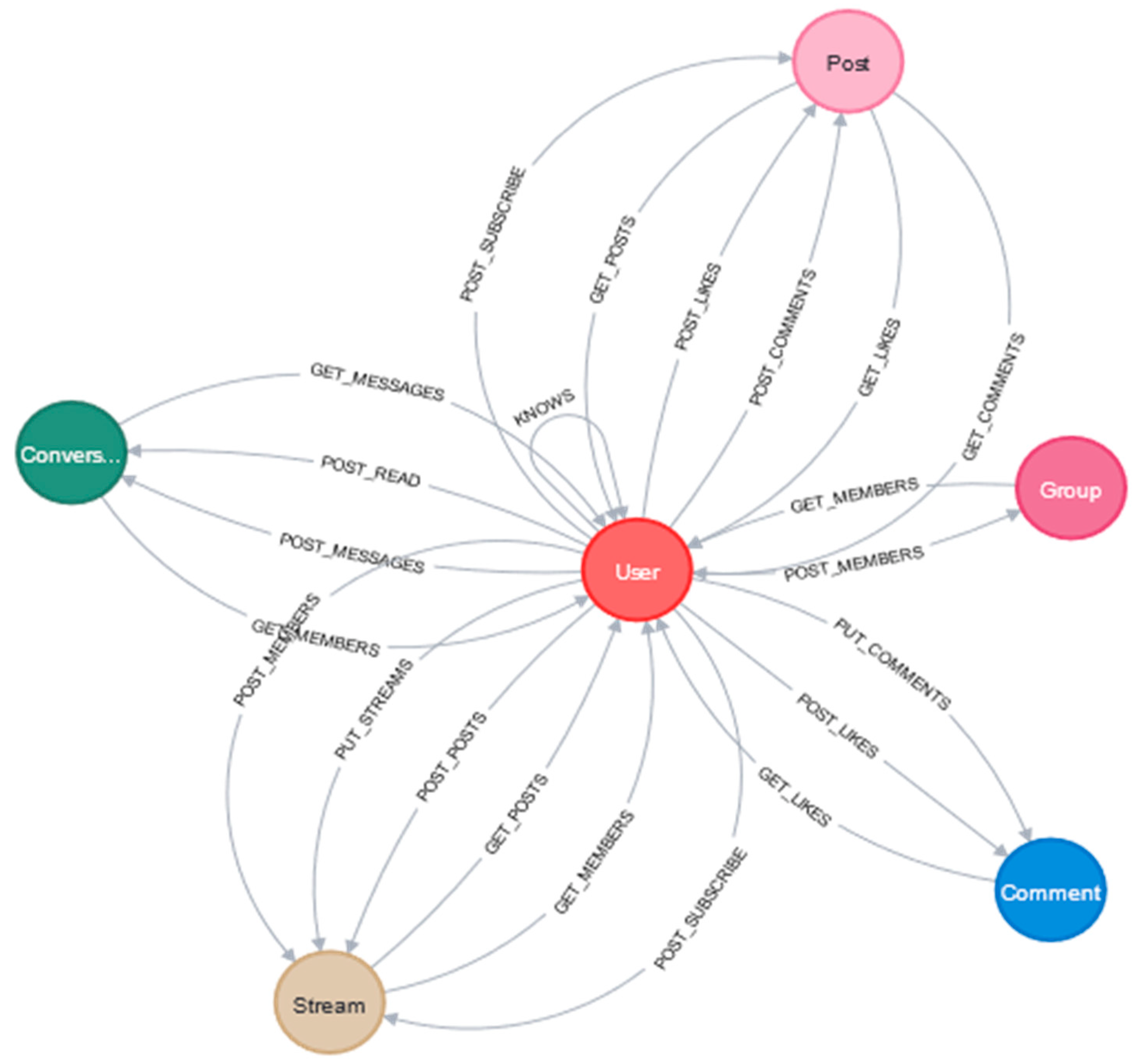
The data frame was loaded with the binary values of the interactions into Neo4j as a CSV file, using various scripts to obtain the predefined data model, which is demonstrated in Figure 1. The properties and data types of the data model are listed in Table 3. The values in the CSV column represent the column names of the CSV file from which the data are loaded into Neo4j. Due to slow performance in Neo4j during the load process, 750.000 rows were used to establish the data model. The properties and data types were set with the Cypher scripts.
The rows of CSV data with KNOWS relationships were loaded into the graph database, where the nodes and relationships were assigned as per the columns. The count property is a dummy value that has the purpose of loading the relationship based on the binary variables in the CSV file.
Weights can be calculated for the relationships between users. However, in this research, relationship weights are not considered because the interest of the work is to extract and predict static relationships. Nevertheless, the data model is designed in such a way that it enables querying of the relationship weights in case of future interest. The graph database includes 5446 nodes and 250,569 relationships in total after the load.
3.4. Exploratory Analysis
After the data transformation, an exploratory analysis was performed on the data. Two main techniques were used: descriptive analysis to learn about the main patterns and extract statistical features from the data. The study also includes the visualization of time series and applying dimensionality reduction techniques with unsupervised machine learning. Since networks change dynamically, the results were only meant for the given sample. The data sample includes 1st January 2019; due to New Year’s wishes, increased user activity is probably present. Thus, this period seems to be suitable to capture several relationships.
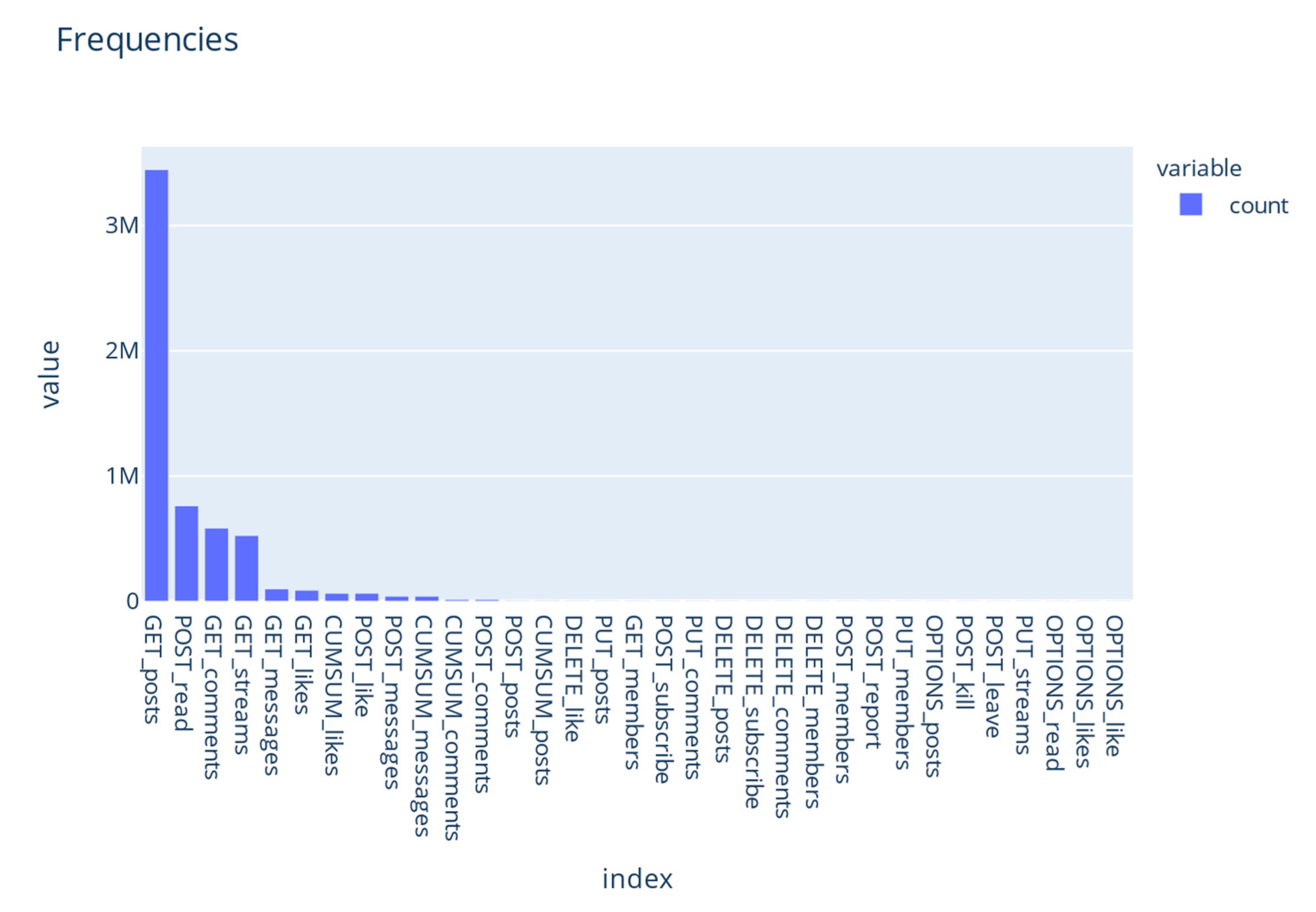
The unsupervised part was performed using Neo4j’s GraphSAGE in-database graph neural network algorithm and the TensorBoard Embedding Projector tool. Table 4 shows an overview of the number of unique values and the frequency of each variable, e.g., that there were 4008 different users in the selected snapshot of the data and who was the most active user. Figure 2 demonstrates that the most frequent user interaction is retrieving posts, as the distribution of the user interactions and the GET_posts is the most common type in the sample. This interaction type means that a user is loading a post. Posts are part of a stream and are visible to all members of the given stream. The users tend to behave passively [30], i.e., they consume information rather than actively responding, sharing, or liking content. Posting likes, comments, etc., is considered active behavior, and the primary active behavior on the network is liking content, which is the POST_like.
Furthermore, Figure 2 indicates that users show relatively passive behavior in their platform usage. The x-axis represents the user interaction, and the y-axis the frequency of the interaction. Interactions starting with CUMSUM and OPTIONS_read, OPTIONS_likes, and OPTIONS_like are not relevant for this research and were further ignored.
3.5. Artifact Design
The artifacts were envisioned based on the research question. The research aims to compare the designed artifacts with which methodology is suitable for applying machine learning algorithms. Artifact 1 aims to extract the current structure of relationships. Artifact 2 demonstrates how in-database link prediction algorithms can be used for graphs. Artifact 3 illustrates the application of machine learning for link predictions as tabular structured data, not graphs. It is important to note that the provided dataset neither has many original features nor does it have categorical variables relevant to the planned artifacts. It means, for tabular data, it must be considered that the prediction for nodes is made in pairs per row, so the model needs pairwise computed features. The Neo4j algorithm considers the graph structure of the data. Thus, individual node features can be used for the model.
3.5.1. Artifact 1: Building Knowledge Graph-Based on User Interaction
This artifact aims to extract the current relationships of users—who knows whom—within Neo4j. The who knows whom type of relationship is not explicitly present on the Beekeeper platform, and second, there is no baseline data to confirm the relationships. It only results in an assumption based on the premise that when two or more users have a conversation, there is a need for information exchange, either personal or professional. Beekeeper could verify whether the two users are in the same department or organizational unit in the company, which helped to determine whether it is likely that they know each other or not. Due to the limitations of the GDPR, this research does not attempt to label the relationship as professional or private between the users. Therefore, only the chat interactions were used, as there is less evidence in other interactions. It cannot be clearly defined whether users liked or commented on the content because they knew the user or were more likely to respond to the content itself. There are interactions in the dataset which did not involve a second user. Those interactions were excluded from the artifact as they could have been caused by the network dynamics not capturing the other user. If the other user did not respond to or never read the message, it is considered irrelevant to Artifact 1.
During the design and prototyping, the user node represents the user, the conversation represents the chat, and the three interactions represent what the user exactly did. The first interaction with the chat item is always GET_messages. This interaction always occurs regardless of whether the user replies or reads the message.
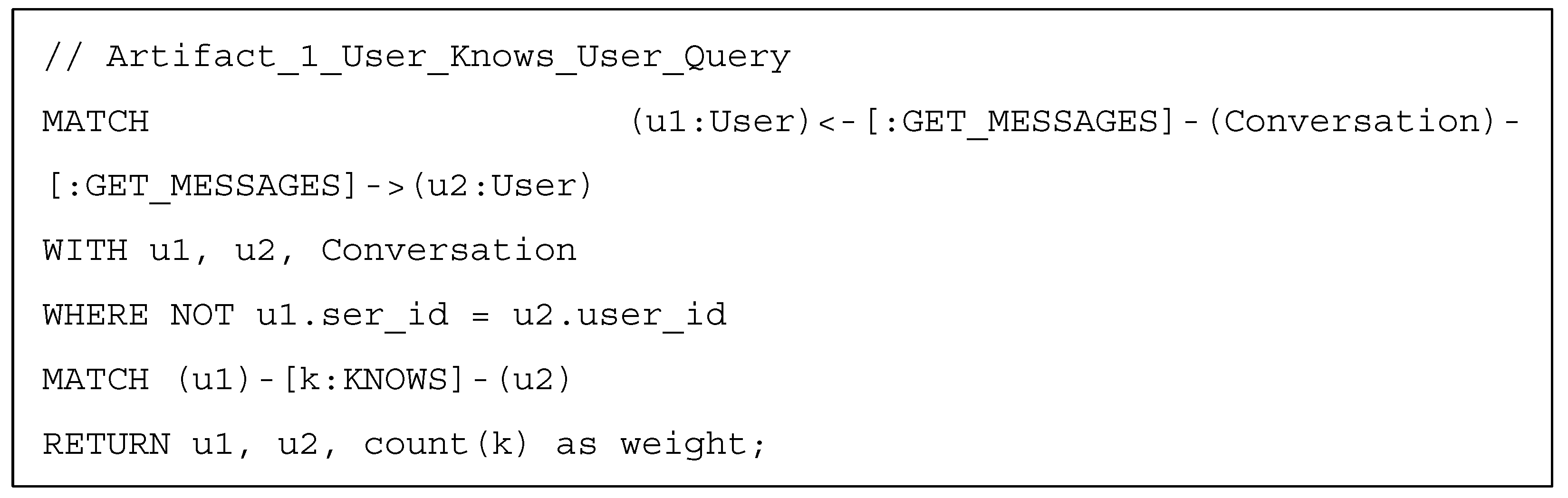
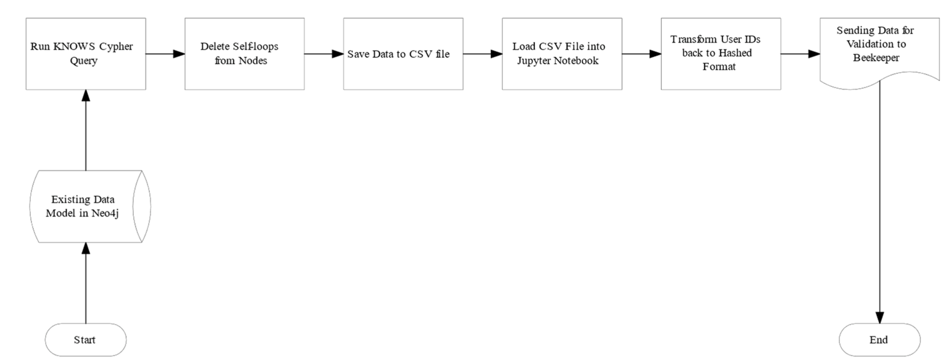
The total number of users in the database was 2819 during the experiment. A query was designed (Figure 3) that resulted in a new relationship, KNOWS, which was written into the database. The extraction of the GET_Messages type of interaction was sufficient to design this artifact since it was the most frequent interaction. These interactions capture that the user is interacting with messages. However, the user is not necessarily reacting to a chat message in the form of a reply. Self-loop relationships are to be excluded from the model since the start and end nodes of the relationship are the same user. These had to be deleted since users are unlikely to ever go into a conversation with themselves. Figure 4 shows the process steps for Artifact 1.
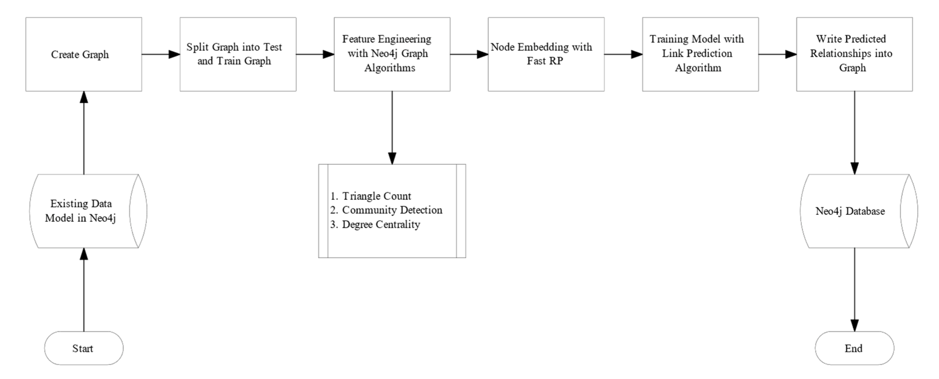
3.5.2. Artifact 2: Link Prediction with Neo4J Graph Machine Learning Algorithms
Artifact 2 represents a predictive model for link prediction using Neo4j’s in-database algorithms. The designed artifact is used to predict user relationships by applying transductive learning and fitting logistic regression to predict probabilities for the user relationship. For prototyping, we used Neo4j’s Graph Data Science Library version 1.7 algorithms. Artifact 2 preserves the graph structure of the data. Training and testing of the models were executed internally in the database, i.e., every transaction happens in the database, and no external algorithms or programming languages were used. The design of the artifact can be divided into eight main steps.
Step 1 is optional. As there might be changes in the data in a production environment, it needs to be ensured that there are no self-loops in the graph. Therefore, deleting the relations KNOWS is essential.
Step 2 is to create an undirected graph with the relationship KNOWS and the label User—the query results in a graph model, which is stored in memory.
Steps 3 and 4 create a training graph and a test graph from the graph model. The graph model is split into a training graph and a test graph. The algorithm labels the relationships, whether they are an existing or not-existing connections between the nodes. The given parameters of the splitting algorithm ensure no overlap between the set of training and testing relationships. Since the ratio of relationships is highly imbalanced due to social networks, the negativeSamplingRatio parameter for class imbalance is 1.0 by default but can also be calculated manually.
The Neo4j documentation summarizes the purpose of relationship splitting as determining the label as positive or negative for each training or test sample. Identify the pair of nodes for which the relationship features are calculated.
Step 5. Engineering a feature using degree centrality. The algorithm uses Freeman’s formula [31] (p. 231) to calculate the centrality of a graph. A single node in an undirected graph is the number of neighbors [31] (p. 220) with which there is a connection. The following equation is used to calculate the degree of nodes, where is a single node and = 1 if and only if and are connected by a line, 0 otherwise.
The equation means the higher the number, the more connections a node has. A value of 0 means, the node is isolated from the network. There are other centrality measures, such as PageRank, eigenvector centrality, or betweenness centrality.
Step 6: Triangle count. The triangle count algorithm [32] is a community detection algorithm determining the number of connected triangles per node in an undirected graph by using the following equation to calculate the triangle count:
The equation results in an integer representing the connection of three nodes, where each node is connected to another. One node can belong to several triangles.
Step 7: Computing Louvain. The Louvain algorithm optimizes the modularity of communities, proposed by a research team at the University of Louvain [33]. The algorithm extracts the hierarchical community structure, meaning one node or even several communities can be a part of several communities, allowing overlaps. The algorithm is considered unsupervised. However, since companies are organized into hierarchical structures, this research dataset contains no information on such structures. The Louvain algorithm might help reveal information about the company’s organizational structure, which can be used to predict relationships.
Step 8 is to apply a node embedding algorithm, which extracts the nodes with their features as vectors. Node embedding algorithms perform two significant actions: first, the network is constructed as a similarity matrix, and second, a dimension reduction technique is applied [34]. The extracted vectors will be used as numerical features to train the link prediction algorithms. Neo4j offers three types of algorithms for node embedding: GraphSAGE [23], Fast Random Projection [34], and Node2vec [24]. Chen et al. found evidence that their proposed Fast Random Projection (Fast RP) algorithm is 4000× faster in computational times than other state-of-the-art algorithms, such as Node2vec or DeepWalk. Here, Fast RP will be used as a node embedding algorithm since it is the only algorithm in production quality offered by Neo4j.
The algorithm optimizes the similarity matrix and utilizes a very sparse random projection. The extended version of the algorithm allows two additional parameters: featureProperties and propertyDimension. The feature properties are the previously computed features such as triangle count and communityId. Table 5 demonstrates the applied parameter values. The feature properties were adjusted; the rest of the parameters remained unchanged and were used as defaults in the documentation.
In step 9, the link prediction algorithm is applied using the node embeddings from step 8. We adjusted the negativeClassWeight parameter to 1 to balance the classes for a 1:1 ratio; validationFold stands for stratified k-fold cross-validation. The concurrency value is the number of threads used to run the algorithm. The penalty is used for logistic regression, indicating how strongly the model should be penalized for misclassifications; 0 is no penalty, and 1 is a very strong penalty. The remaining parameters were used as specified in the product documentation [35]. Table 6 summarizes the parameters that were used with the link prediction algorithm.
The link prediction algorithm fits a logistic function and sigmoid function with values between 0 and 1. Logistic regression predicts the probability of the label for a given input variable. The threshold is 0.45 for a provided label, i.e., if the probability is less than 0.45, the label is predicted to be 0. Otherwise, it is expected to be 1.
Figure 5 demonstrates the process steps described for prototype Artifact 2. The predicted positive relationships are written back into the database. These can be visualized with Neo4j Bloom or downloaded in a JSON or CSV format. The topN parameter defines the top 30 relationships, and the threshold determines the probability score above which the relationships are returned, in this case, 0.45. However, both topN and the threshold are arbitrary.
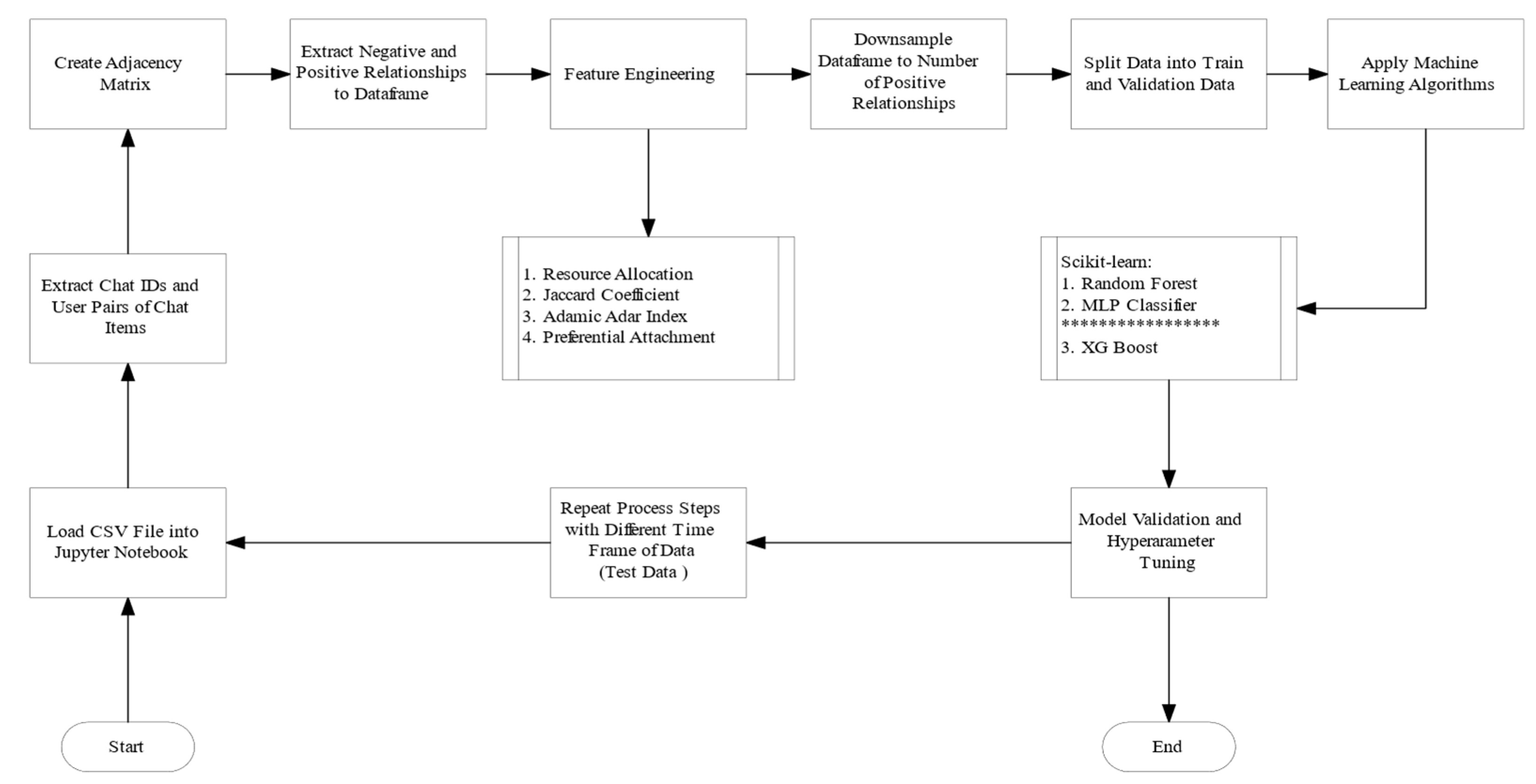
3.5.3. Artifact 3: Link Prediction for User Relationships with Scikit-Learn
The purpose of Artifact 3 is to create a predictive model for link prediction using scikit-learn. This artifact demonstrates a model architecture for machine learning without using Neo4j.
By taking a different approach in the design, this artifact treats the data as tabular and makes the predictions pairwise for the nodes. Therefore, the model requires different features than Artifact 2. They need to be engineered for the node pairs. Python is used as the main programming language for prototyping, feature engineering, NetworkX, and predictive modeling with the scikit-learn libraries. The first 15,000,000 rows were loaded for the training model, and the test set was created from the 15,000,001–30,000,000 rows.
Step 1 is a recap of the transformation steps. The data were transformed to split the API path into columns and label-encoded the user IDs as variables for easier handling. The dataset was filtered only for the variable conversations where only one user was in the chat. The users were paired based on conversation ID, and since only the relationship link and not the weighting was of interest, only the first interaction of the conversation was retained. The resulting data frame contains the two user IDs and the conversation ID. The column weights are not further considered.
Step 2 uses NetworkX and matrices to prepare the dataset for predictive modeling. NetworkX is used to create an undirected graph from the resulted data frame of step 1. This graph is converted next into an adjacency matrix to be able to extract negative and positive relationships.
The binary values of the adjacency matrix will be the labels of the dataset for the predictive modeling. The matrix is converted into a data frame with each user pair’s extracted 0 or 1 label. The self-connections, for example, 1 to 1 and duplicated relationships, were excluded from the data frame as it does not matter whether 1 knows 2 or 2 knows 1; the relationship is required to be captured only once. Because self-relationship provides no valuable information for the model, these values were also excluded.
Step 3 is engineering features, as only features for pairwise scores are considered for the model since the data are treated as tabular data. The features are engineered with the algorithms of the NetworkX library, under the link prediction algorithms [36]. We selected the following algorithms for feature engineering:
Preferential attachment. Preferential attachment is a probabilistic algorithm that calculates the probability that a new node will connect to another node based on the number of its connections [37].
The algorithm uses the following formula, where is the degree of the i-th node:
Resource allocation index. The resource allocation index is a similarity-based measurement algorithm indicating the proximity of two pairs of nodes [38] by using the following equation, where x and y are not directly connected, where Γ(x) is the set of neighbors of node x, and k(z) the degree of the common neighbor nodes:
If the result of the equation is close to 0, it means the nodes are not close to each other.
Jaccard coefficient. The Jaccard coefficient is a similarity measure defined by Paul Jaccard. It compares the number of shared neighbors with the total number of neighbors of the two nodes indicated by A and B in the equation:
The result can have a value between 0 and 1; the closer the number is to 1, the more similar the nodes are.
Adamic–Adar index. The Adamic–Adar algorithm is a similarity-based measure calculating the proximity of nodes by logarithmizing the degrees of common nodes of x and y [39]. The formula of the resource allocation index is very similar to that of Adamic and Adar [38]. Zhou et al. pointed out that the difference between the two indices is insufficient in the case of a small degree, but when the degree in the network is large, the resource allocation index performs better.
The listed algorithms are all available in the NetworkX library. The four features are computed for each node pair; the results of the algorithms are stored in a data frame. The last step is to merge all the data frames into one, resulting in the user pairs, four feature columns, and a label column with 0 and 1.
In step 4, the data are downsampled based on the matrix from step 2. The node pairs with 0 labels are randomly resampled to the same number as the positive samples. Downsampling was necessary because the data set was unbalanced due to the high number of non-connections between nodes. Applying downsampling may result in pattern loss, but otherwise, the model would conclude that there are mainly no relationships between users and would fail to learn to predict the positive ones.
Step 5 is the construction of the predictive machine learning model with scikit-learn. Only Random Forest Classifier is discussed because it performed better than the other algorithms. Random Forest [40] is an ensemble learning method used for binary classification in this context, and belongs to the family of decision tree algorithms. The working mechanism of random forest is that individual models are trained with bootstrap sampling for prediction, forming an ensemble of trees. In the end, the main class determines the winning label for the model by voting. Random forests have gained popularity within the machine learning community because they are robust, perform well on large datasets, and handle many variables. The negative point is that they are sensitive to unbalanced classes, as the tuning of hyperparameters will likely lead to overfitting the model. Figure 6 demonstrates the process steps of Artifact 3.
4. Results
4.1. Resulting Artifacts
4.1.1. Artifact 1: Who knows who Knowledge Graph
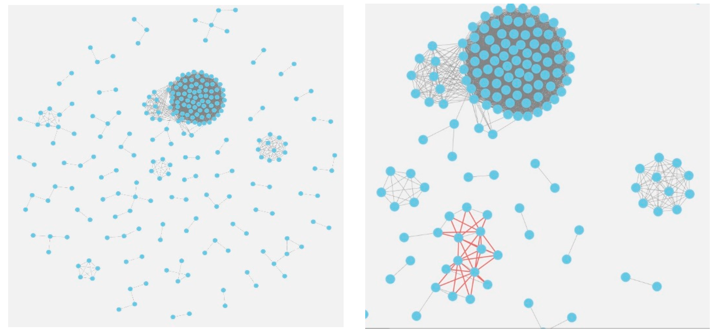
Based on the chat interactions, the first resulting artifact is a labeled property graph created by Neo4j that shows who knows whom in the network. The visual layer of the artifact is represented with Neo4j Bloom in Figure 7. The resulting query can be saved in a JSON and CSV file format, meaning the users and their relationships. Filtering of the individual users or different coloring of the nodes is possible. Non-existing connections are not displayed in the tabular representation, only the positive ones.
4.1.2. Artifact 2: Link Prediction using Neo4j in-Database Algorithms
The second resulting artifact is a predictive machine learning model using Neo4j in-database algorithms. The visual representation of the results was done using Neo4j Bloom, which displays the predicted relationships (see Figure 7). The database contains 2819 user nodes, which were used to build the model. Artifact 2 is a probabilistic model providing the 30 highest predicted probabilities. They are above the defined threshold of 0.45. In other words, the red lines in Figure 7 represent predicted relationships where the probability value is above 0.45, indicating that users know each other, and these are written as different relationships in the graph. With Neo4j Bloom, the KNOWS_PREDICTED relationship is visualized on the layer of artifact 1 to better understand where the predicted relationships are located within the network. The prediction probability is the same for both users, i.e., with an undirected graph, the direction is not considered. Hence, the probability value is the same regardless of whether user A knows user B or vice versa. Therefore, there are two arrows for one relationship in the visualization in Neo4j Bloom. The resulted visualization can be exported in different formats, for example, CSV, JSON, or PNG.
4.1.3. Artifact 3: Link Prediction with Scikit-Learn
The third resulting artifact is a predictive machine learning model with scikit-learn using its Random Forest Classifier algorithm. The model is called the Train Model. The model was trained on a downsampled dataset with 3605 positive and 3605 negative samples, using a mixed split ratio of 80:20 for the training and validation set. A grid search was applied to look for the best model parameter that reached the highest accuracy. These parameters were used with the test dataset to evaluate the model’s performances with accuracy, precision, and recall metrics. These metrics are built-in. The prediction result is a vector with values between 0 and 1, representing the predicted classes for the user pairs. Optionally, the model can return probability scores instead of binary categories. The main reasons the random forest algorithm over the neural network was preferred were its architecture and tuning of the parameters. Finding the best performing model for a neural network requires much more parameter knowledge than random forests. Therefore, neural networks may perform better in academia. Still, for production implementation, random forest is likely the better choice because the results are easier to understand and explain to a broad audience how they work.
4.2. Evaluation of Artifacts
Several evaluation metrics were used for the machine learning models, with metrics for precision, recall, accuracy, and area under the curve (AUC). Beekeeper was asked to provide feedback on the relationships sampled from Artifact 1, and the prediction results for Artifact 2 and Artifact 3.
Evaluating the artifacts with ground truth data in the customer tenant allows a better understanding of model quality and improvement of data labels. The evaluation was done based on the labeling of Beekeeper on the predicted user relationship types. The relationships from Neo4j were downloaded in CSV format. This CSV file was formatted to extract the user IDs and weights from the string values in three columns. Since the user IDs are hashed in the original format, the user IDs used in Neo4J were “mapped back” to the original hashed IDs.
The validation sample included 3373 users, including the user pairs, depending on the artifact, the probability score, and predicted classes. Beekeeper assigned to these user pairs the job position division, business unit, user status, and relationship type. The column status of the users means whether a user is still an active user or has been suspended. The relationship type is in the validation column, indicating the users’ relationship: cross-departmental communication, colleagues’ interaction, manager interaction, security report, or unknown. We received the validation file from Beekeeper on 2 December 2021.
The precision-recall area under the curve (AUCPR) displays the precision and recall variety at different thresholds, and the goal is to have the area under the PR curve maximized, which represents a good classifier model.
Precision (P) is defined as the number of true positives over the number of true positives plus the number of false positives :
Recall (R) is defined as the number of true positives over the number of true positives plus the number of false negatives :
The so-called baseline average precision mean score (AP) has a value of 0.5, and the perfect classifier 1. Under 0.5, the classifier is not considered performant. The AP is calculated with the following equation:
Accuracy is a good measure when classes are balanced, but a social network usually has fewer existing connections than non-existing connections, so AUCPR is a more appropriate metric for evaluation. Neo4j can only return AUCPR as an evaluation metric, so Artifact 3 was also evaluated using the precision-recall curve to compare the results. Since the data were balanced, accuracy as a metric is applicable. However, balancing the data required a trade-off for pattern loss, which must be considered when interpreting the results.
4.2.1. Evaluation of Artifact 1
The sample included 300 users for Artifact 1, which was sent to Beekeeper to validate the user relationships, whether the users knew each other or not.
The resulted model is time-dependent, and the captured network structure could be different in a different time frame, such as during the vacation or vacation season.
The validation by Beekeeper confirmed that out of 300 relationships, 278 exist. Twenty-two relationships could not be found in the system. Almost one-third of the validated relationships were classified as incident reporting. Interesting is the unknown relationship status because these users had chat interaction. However, there is no evidence that they would know each other in the system. Looking at whether the users were suspended, only 2 relationships out of 22 are unknown because of the suspended status.
4.2.2. Evaluation of Artifact 2
We first evaluated with the AUCPR metric using cross-validation defined in the validationFolds stem parameter, so no separate validation dataset has been used for the model. Furthermore, the data contained only one week of time lag. Therefore, creating an additional validation set besides the test and training split would not have been meaningful. Hence, 120 user relationships were sent to Beekeeper for validation.
Table 7 represents the results of the Link Prediction algorithm extracted from the Neo4j Desktop. TrainGraphScore here means the AUCPR score. The results for prediction might be saved either as CSV or in JSON format. The algorithm returns the winning model with the penalty and epoch values, along with the highest train and test scores. The epoch stands for how many times the data has been trained, and the penalty is the value for the L2 regularization.
The predicted results can be streamed with the stream mode of the link prediction algorithm, allowing the extraction of node pairs and predicted connections. Then, the streamed user pairs were provided again to Beekeeper for further validation, to determine whether more evidence could be found that these connections exist in the client’s system.
The test graph scores 0.344, indicating that the model performs moderately poorly overall, but it is considered acceptable due to the absence of the original features.
Beekeeper’s validation of predicted relationships confirms that all the relationships are accurate and exist in the system. Thus, although the predictive models have an average low AUCPR score, they are performing well from a business domain perspective, as all the relationships exist, and there are no unknown labels. However, the data sent to Beekeeper for validation contained 60 duplicated user pairs, which means only 60 out of 120 users could be considered.
The model predicted relationships with colleagues’ interaction labels with the highest number of user pairs: 56. Followed by security reports with 48 user pairs, and manager interaction with the lowest number of user pairs, with 16.
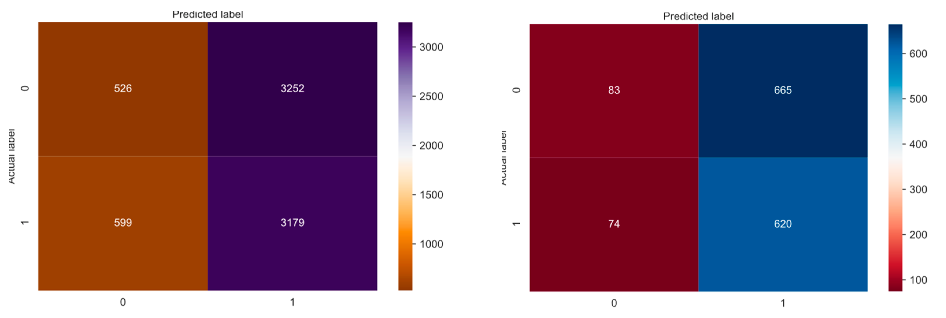
4.2.3. Evaluation of Artifact 3
Artifact 3 was evaluated with the visual observation of the precision-recall curve of the Train Model and its confusion matrix, using 5-fold cross-validation for the grid search. After the data transformation, the test dataset included 7556 samples, with 3778 negative and 3778 positive relationships. Using a test dataset ensures that, in the case of model tuning based on the results with the validation data, the tuned model can be evaluated with unseen data. The test dataset was created using the original dataset’s 15–30 million rows.
The correlation matrix (see Table 8) of the downsampled features shows no strong linear correlation between the variables. We computed it on the data frame of the Train Model before splitting the data into test and train sets. The strongest positive correlation between the resource allocation index and the Adamic–Adar index is reasonable due to the similarity of the underlying mathematics of the algorithms. The Jaccard similarity score has the lowest correlation coefficient with the other features. There is no negative correlation present in the model’s feature set.
Random forests and other decision tree-based algorithms are not affected by multicollinearity [41] (p. 268). Therefore, the features can be used in the current setup without further testing multicollinearity.
Figure 8 shows that the model classifies a lot of false positives, although the classes have been balanced. Looking at the precision-recall curves of both datasets, we see the precision values decrease with an increasing recall rate, and after a specific value, they seem to be more balanced, taking the value of 0.5.
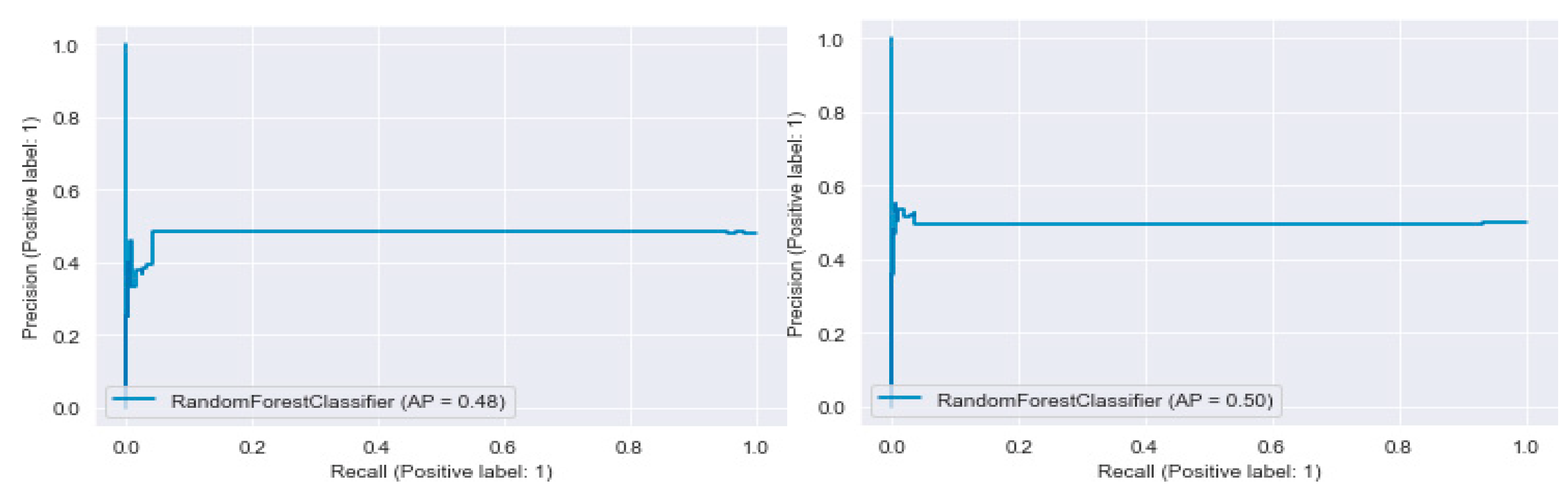
Figure 9 represents the PR curve of the Train Model for prediction on the validation dataset with the random forest classifier. The plot shows that the classifier is performing at its baseline. The model’s performance with the test dataset uses the random forest classifier. The average precision score (AP) is 0.51, which can be considered moderate for both models. The visual representation of the PR curves shows evidence that the classifier is not performing better than random guessing and is performing well only at a low recall rate, meaning the returned results are precise; however, the number of these values is only a few.
Max_Depth determines the depth of the tree, and N_Estimators are the maximum number of trees to grow. Table 9 displays the model results with the maximum accuracy and AUC, returning their hyperparameters and the highest probability score found with grid search. The difference between AUC and accuracy is that the AUC considers the probability scores of the predictions, while accuracy considers the correctness of the predicted classes. Accuracy is, in this case, applicable because the classes were balanced out. However, the precision-recall metrics are more appropriate for implementing the algorithm in a production environment due to the class imbalance in real-life data.
Although the hyperparameters are different, the best scores, the mean best scores of the cross-validation, are similar for both datasets.
Table 10 demonstrates the results of the model metrics with the validation and test datasets of the Train Model. The high recall rate means that our model is predicting the true positive classes well, but the low precision rate indicates the high number of false positives, which we have seen in the confusion matrices.
Table 11 displays the key comparative numerical aspects of Artifact 2 and Artifact 3. The validation results by Beekeeper will be in the Discussion chapter of this work. The average precision (AP Score) in scikit-learn is the same metric as the AUCPR score yielded by the algorithm of Neo4j. Therefore, based on these metrics, the average precision of the two artifacts is comparable.
5. Discussion
5.1. Insights from the Artifact Evaluation
Analyzing the feature quality revealed that using node embeddings for predictive models is likely more suitable, as engineered numerical features have been primarily zeros. Artifacts 1 and 2 have demonstrated their advantages for visualizing using a graph database, and Artifact 3 has presented an alternative solution without using a graph database. The two approaches to link prediction were compared, one as a graph and the other as tabular data, showing the similarities and differences between the advantages and disadvantages of the models.
We compared the performance of Artifact 2 (link prediction using Neo4j Graph Data Science Library, GDSL) with Artifact 3 (link prediction using scikit-learn). Neo4j only allowed AUC as a measure, which can be considered an average precision where the average is over different classification thresholds. In terms of AUC, Artifact 3 is better. However, the precision of Artifact 3 is still random (50%) in the balanced dataset because the baseline probability is 50%. This means that the prediction is not useable in practice. Additionally, we observed that Artifact 3 is much slower in computation time. We noticed that Artifact 3 uses relationship features between nodes instead of individual node features. It compares the set of standard user interactions (chats). However, it is clear that better, more selective features need to be found, either structurally or by looking at the actual content.
5.2. Lessons Learned in the Study Case (Beekeeper)
The work presented in this research has a relevant impact on Beekeeper’s business direction and the potential development of future features around user behavior.
GDPR data has consistently added value to the Beekeeper business model since the company guarantees total privacy to its users. However, it also represents a limitation to improving user experience through simple recommendations or analyzing user behavior for the purpose of understanding the final users better because the company cannot openly analyze the user data without their consent.
This study shows the first milestones to understanding users’ behavior at Beekeeper under a GDPR context. It shows the need to find a balance between privacy and user data consent to reach higher levels of precision. Moreover, this opens the door to developing potential strategies to convince customers to provide consent to improve Beekeeper services.
Beekeeper keeps closer contact with its customers through a customer success department, which empowers users to provide constant feedback and identify valuable use cases that may qualify to be implemented as a new feature in Beekeeper.
Once a potential use case or feature qualifies for development, there is a need to discover a prototype or proof of concept. This happens typically in the industry in two phases:
- Outsourcing the prototype to industry partners and consultants such as Price Waterhouse Coopers, Accenture, etc.
- Internal research and development or prototyping through an academic partner.
In practice, outsourcing the prototype leads to more costs since integration partners add a tag price on the advisory services and implementation and push the negotiation to have a percentage of the revenue generated by the newly implemented feature. This is a natural effect in industry collaborations or partnerships to justify the costs of allocating resources on both sides. However, the latter mostly happens when the client does not know how a new technology works.
In practice, Beekeeper has noticed the benefits of exploring potential proofs of concepts in advance with academic partners, leading to internal know-how. This enables the company to collect more feedback from end-users. In other words, it enables Beekeeper to fine-tune potential new features several times in a cost-effective way.
Once the feature gains maturity and is ready to be implemented, it may be outsourced to industry partners or consultants. Nevertheless, the requirements are more precise, which saves costs in prototyping and human capital expertise in the long run.
Developing know-how in advance allows startups or companies such as Beekeeper with limited human expertise resources to have a better negotiation position with partner integrators or consultants since the limitations, risks, and disadvantages are mostly known in advance. Therefore, it leads to a more effective solution and collaboration.
5.3. Summary and Outlook
The article compared two different approaches to predicting user relationships in an enterprise social network without knowing the content, only by evaluating the graph structure. The main objective of this research was to find evidence of whether machine learning can be applied to GDPR-compliant data with accurate results. The study provided descriptive insights using statistical analysis and used experiments to show potential ways for predictive modeling of user relationships.
Our further recommendation is to try different features and run the models on other customers’ data or time frames. Combining StellarGraph with Keras delivered promising results when combined with Neo4j node embeddings. Therefore, experimenting with graph neural networks was suggested for future research.
This study offered many lessons in the application of graph mining and added to know-how development, but the predictive results were below expectations. More research is needed in feature engineering and selection for link prediction based on structural graph features that anonymize and hide content. Behavioral modelling, liking, and commenting activities could be considered as future research topics. Commonly linked nodes for other types of interactions (posts, likes, comments) as features should also be studied.
Author Contributions
R.K.: Experiments, analysis, and prototype implementation as part of her master’s thesis, M.K.: Research design, interpretation, guidance, manuscript structure, conclusions, outlook, and further research, J.A.M.: Data analysis, experiments’ interpretation, Beekeeper business perspective, data anonymization, data extraction, and data validator with the Beekeeper customer to enable Artifact 2 and 3 evaluations. All authors have read and agreed to the published version of the manuscript.
Funding
Beekeeper provided financing to give GDPR-compliant data for this research study and extra hours of data engineering to extract the needed information from the core Beekeeper cloud solution through a series of anonymization steps.
Data Availability Statement
The primary RAW dataset and files to reproduce the study can be found at https://zenodo.org/record/6309436#.Yh0a_hPMIeZ.
Conflicts of Interest
The authors declare no conflict of interest.
References
- Boyd, D.M.; Ellison, N.B. Social Network Sites: Definition, History, and Scholarship. J. Comput.-Mediat. Commun. 2007, 13, 210–230. [Google Scholar] [CrossRef] [Green Version]
- Heim, S.; Yang, S. Content Attractiveness in Enterprise Social Networks. In Proceedings of the 2nd European Conference on Social Media (ecsm 2015), Porto, Portugal, 9–10 July 2015; pp. 199–206. Available online: https://www.webofscience.com/wos/woscc/full-record/WOS:000404225700025 (accessed on 11 October 2021).
- Wang, P.; Xu, B.; Wu, Y.; Zhou, X. Link Prediction in Social Networks: The State-of-the-Art. arXiv 2014, arXiv:physics/1411.5118. Available online: http://arxiv.org/abs/1411.5118 (accessed on 29 March 2021). [CrossRef] [Green Version]
- Rajaraman, A.; Ullman, J.D.; Leskovec, J. (Eds.) Mining Social-Network Graphs. In Mining of Massive Datasets, 2nd ed.; Cambridge University Press: Cambridge, UK, 2014; pp. 325–383. [Google Scholar] [CrossRef] [Green Version]
- Beekeeper—The Secure Employee App. Beekeeper. Available online: https://www.beekeeper.io/en/home-copy/ (accessed on 1 June 2021).
- Liben-Nowell, D.; Kleinberg, J. The link-prediction problem for social networks. J. Am. Soc. Inf. Sci. Technol. 2007, 58, 1019–1031. [Google Scholar] [CrossRef] [Green Version]
- Meske, C.; Wilms, K.; Stieglitz, S. Enterprise Social Networks as Digital Infrastructures-Understanding the Utilitarian Value of Social Media at the Workplace. Inf. Syst. Manag. 2019, 36, 350–367. [Google Scholar] [CrossRef] [Green Version]
- Drahošová, M.; Balco, P. The Benefits and Risks of Enterprise Social Networks. In Proceedings of the 2016 International Conference on Intelligent Networking and Collaborative Systems (INCoS), Ostrava, Czech Republic, 7–9 September 2016; pp. 15–19. [Google Scholar] [CrossRef]
- Luo, N.; Guo, X.; Lu, B.; Chen, G. Can non-work-related social media use benefit the company? A study on corporate blogging and affective organizational commitment. Comput. Hum. Behav. 2018, 81, 84–92. [Google Scholar] [CrossRef]
- Fortunato, S. Community detection in graphs. Phys. Rep. 2010, 486, 75–174. [Google Scholar] [CrossRef] [Green Version]
- Yang, Z.; Algesheimer, R.; Tessone, C.J. A Comparative Analysis of Community Detection Algorithms on Artificial Networks. Sci. Rep. 2016, 6, 1–18. [Google Scholar] [CrossRef] [Green Version]
- Ding, Z.; Zhang, X.; Sun, D.; Luo, B. Overlapping Community Detection based on Network Decomposition. Sci. Rep. 2016, 6, 24115. [Google Scholar] [CrossRef] [Green Version]
- Rosvall, M.; Delvenne, J.-C.; Schaub, M.T.; Lambiotte, R. Different approaches to community detection. arXiv 2019, arXiv:Physics/1712.06468. [Google Scholar] [CrossRef] [Green Version]
- Newman, M.E.J. Modularity and community structure in networks. Proc. Natl. Acad. Sci. USA 2006, 103, 8577–8582. [Google Scholar] [CrossRef] [Green Version]
- Harush, U.; Barzel, B. Dynamic patterns of information flow in complex networks. Nat. Commun. 2017, 8, 2181. [Google Scholar] [CrossRef] [Green Version]
- Zareie, A.; Sakellariou, R. Similarity-based link prediction in social networks using latent relationships between the users. Sci. Rep. 2020, 10, 20137. [Google Scholar] [CrossRef]
- Menon, A.K.; Elkan, C. Link Prediction via Matrix Factorization. In Machine Learning and Knowledge Discovery in Databases; Gunopulos, D., Hofmann, T., Malerba, D., Vazirgiannis, M., Eds.; Springer: Berlin/Heidelberg, Germany, 2011; Volume 6912, pp. 437–452. [Google Scholar] [CrossRef] [Green Version]
- Barabási, A.-L.; Pósfai, M. Network Science; Cambridge University Press: Cambridge, UK, 2016; Available online: http://barabasi.com/networksciencebook/ (accessed on 5 November 2021).
- Broido, A.D.; Clauset, A. Scale-free networks are rare. Nat. Commun. 2017, 10, 1017. [Google Scholar] [CrossRef]
- Algorithms—Neo4j Graph Data Science. Neo4j Graph Database Platform. Available online: https://neo4j.com/docs/graph-data-science/1.7/algorithms/ (accessed on 15 October 2021).
- Panagopoulos, G.; Nikolentzos, G.; Vazirgiannis, M. Transfer Graph Neural Networks for Pandemic Forecasting. arXiv 2021, arXiv:2009.08388. Available online: http://arxiv.org/abs/2009.08388 (accessed on 15 October 2021).
- Hamilton, W.L.; Ying, R.; Leskovec, J. Inductive Representation Learning on Large Graphs. arXiv 2020, arXiv:1706.02216. Available online: http://arxiv.org/abs/1706.02216 (accessed on 13 December 2020).
- Hamilton, W.L.; Ying, R.; Leskovec, J. Representation Learning on Graphs: Methods and Applications. arXiv 2017, arXiv:1709.05584. [Google Scholar]
- Grover, A.; Leskovec, J. node2vec: Scalable Feature Learning for Networks. arXiv 2016, arXiv:1607.00653. Available online: http://arxiv.org/abs/1607.00653 (accessed on 15 April 2021).
- Fast Random Projection—Neo4j Graph Data Science. Neo4j Graph Database Platform. Available online: https://neo4j.com/docs/graph-data-science/1.7/algorithms/fastrp/ (accessed on 15 October 2021).
- Li, M.; Wang, X.; Gao, K.; Zhang, S. A Survey on Information Diffusion in Online Social Networks: Models and Methods. Information 2017, 8, 118. [Google Scholar] [CrossRef] [Green Version]
- Graph Classification—StellarGraph 1.2.1 Documentation. Available online: https://stellargraph.readthedocs.io/en/stable/demos/graph-classification/ (accessed on 15 October 2021).
- Österle, H.; Becker, J.; Frank, U.; Hess, T.; Karagiannis, D.; Krcmar, H.; Loos, P.; Mertens, P.; Oberweis, A.; Sinz, E.J. Memorandum Zur Gestaltungsorientierten Wirtschaftsinformatik. Available online: http://www.alexandria.unisg.ch/Publikationen/71074 (accessed on 5 May 2021). (In German) [CrossRef]
- Géron, A. Hands-On Machine Learning with Scikit-Learn, Keras, and TensorFlow, 2nd ed.; O’Reilly Media, Inc.: Newton, MA, USA, 2019; Available online: https://www.oreilly.com/library/view/hands-on-machine-learning/9781492032632/ (accessed on 5 December 2021).
- Escobar-Viera, C.G.; Shensa, A.; Bowman, N.D.; Sidani, J.E.; Knight, J.; James, A.E.; Primack, B.A. Passive and Active Social Media Use and Depressive Symptoms Among United States Adults. Cyberpsychol. Behav. Soc. Netw. 2018, 21, 437–443. [Google Scholar] [CrossRef]
- Freeman, L.C. Centrality in social networks conceptual clarification. Soc. Netw. 1978, 1, 215–239. [Google Scholar] [CrossRef] [Green Version]
- Becchetti, L.; Boldi, P.; Castillo, C.; Gionis, A. Efficient semi-streaming algorithms for local triangle counting in massive graphs. In Proceedings of the 14th ACM SIGKDD International Conference on Knowledge Discovery and Data Mining, Las Vegas, NV, USA, 24–27 August 2008; Association for Computing Machinery: New York, NY, USA; pp. 16–24. [CrossRef] [Green Version]
- Blondel, V.D.; Guillaume, J.-L.; Lambiotte, R.; Lefebvre, E. Fast unfolding of communities in large networks. J. Stat. Mech. 2008, 2008, P10008. [Google Scholar] [CrossRef] [Green Version]
- Chen, H.; Sultan, S.F.; Tian, Y.; Chen, M.; Skiena, S. Fast and Accurate Network Embeddings via Very Sparse Random Projection. arXiv 2019, arXiv:1908.11512. Available online: http://arxiv.org/abs/1908.11512 (accessed on 21 October 2021).
- Link Prediction—Neo4j Graph Data Science. Available online: https://neo4j.com/docs/graph-data-science/1.7/algorithms/ml-models/linkprediction/ (accessed on 5 November 2021).
- Link Prediction—NetworkX 2.6.2 Documentation. Available online: https://networkx.org/documentation/stable/reference/algorithms/link_prediction.html (accessed on 16 November 2021).
- Barabasi, A.L.; Albert, R. Emergence of scaling in random networks. Science 1999, 286, 509–512. [Google Scholar] [CrossRef] [Green Version]
- Zhou, T.; Lu, L.; Zhang, Y.-C. Predicting Missing Links via Local Information. Eur. Phys. J. B 2009, 71, 623–630. [Google Scholar] [CrossRef] [Green Version]
- Adamic, L.A.; Adar, E. Friends and neighbors on the Web. Soc. Netw. 2003, 25, 211–230. [Google Scholar] [CrossRef] [Green Version]
- Breiman, L. Random Forests. Mach. Learn. 2001, 45, 5–32. [Google Scholar] [CrossRef] [Green Version]
- Kotsiantis, S.B. Decision trees: A recent overview. Artif. Intell. Rev. 2013, 39, 261–283. [Google Scholar] [CrossRef]
Figure 1.
Data Model in Neo4j.

Figure 2.
Frequencies of User Interactions.

Figure 3.
Cypher Query “who knows who”.

Figure 4.
Process Diagram for Artifact 1.

Figure 5.
Process Diagram for Artifact 2.

Figure 6.
Process Diagram for Artifact 3.

Figure 7.
Labeled Property Graph Visualized with Neo4j Bloom (left) and Predicted Relationships with Link Prediction (right). Screenshot from Neo4j Bloom of the USER-KNOWS-USER query.
Figure 7.
Labeled Property Graph Visualized with Neo4j Bloom (left) and Predicted Relationships with Link Prediction (right). Screenshot from Neo4j Bloom of the USER-KNOWS-USER query.

Figure 8.
Confusion Matrix of Train Model with Validation Dataset (left) and Test Dataset (right), based on subsampling of chat interactions.
Figure 8.
Confusion Matrix of Train Model with Validation Dataset (left) and Test Dataset (right), based on subsampling of chat interactions.

Figure 9.
Precision-Recall Curve of Train Model on Validation Dataset (left) and Test Dataset (right).
Figure 9.
Precision-Recall Curve of Train Model on Validation Dataset (left) and Test Dataset (right).


Table 1.
Variable Names and Types of Original Dataset.
| Variable Name | Description | Data Type |
|---|---|---|
| _inserted_at | The time of insert into the database | Datetime |
| id | Anonymized ID of the interaction | String |
| occurred_at | The time of user interaction happened | Datetime |
| user_id | Anonymized ID of the user | String |
| is_bot | True or False whether the interaction was performed by a bot | Boolean |
| client | Client of user device | String |
| client_version | Client version of user device | String |
| path | API endpoint of interaction | String |
| normalized_path | Normalized API endpoint | String |
| method response_status | HTTP Response Status Code | String |
| turnaround_time | Turnaround time | String |
Table 2.
Selected Variables Based on Data Model.
| Variable Name | Description | Data Type |
|---|---|---|
| occured_at | The time the user interaction happened | Datetime |
| user_id | Anonymized ID of the user | Integer |
| client | Client of user device | Integer |
| path | API endpoint of interaction | String |
| normalized_path | Normalized API endpoint | String |
Table 3.
Data Model Node Details.
| Node Type | Property | CSV Column | Data Type |
|---|---|---|---|
| Post | post_id | posts | Integer |
| User | user_id | user_id | Integer |
| Group | group_id | groups | Integer |
| Comment | comment_id | comments | Integer |
| Stream | stream_id | streams | Integer |
Table 4.
Statistical Overview of the Dataset Sample (First 15 million records).
| User_Id | Client | Client_Version | Path | Normalized Path | Method | |
|---|---|---|---|---|---|---|
| unique | 4008 | 5 | 45 | 138835 | 150 | 6 |
| top | - | app-ios | 4.23.6b49 | /status | /{streamid}/posts | GET |
| freq | 104637 | 8664127 | 8551708 | 1607679 | 2770088 | 12943606 |
Table 5.
Parameters Used for the Fast RP Algorithm.
| Parameter Name | Parameter Value |
|---|---|
| propertyDimension | 45 |
| embeddingDimension | 250 |
| featureProperties | [“communityId”, “triangles”, ‘degree’], |
| relationshipTypes | [“KNOWS_REMAINING”] |
| iterationWeights | [0, 0, 1.0, 1.0] |
| normalizationStrength | 0.05 |
| mutateProperty | ‘fastRP_Embedding_Extended’ |
Table 6.
Link Prediction Model Parameters.
| Parameter Name | Parameter Value |
|---|---|
| trainRelationshipType | ‘KNOWS_TRAINGRAPH’ |
| testRelationshipType | ‘KNOWS_TESTGRAPH’, |
| modelName | ‘FastRP-embedding |
| featureProperties | [fastRP_Embedding_Extended], |
| validationFolds | 5 |
| negativeClassWeight | 1.0 |
| randomSeed | 2 |
| concurrency | 1 |
| params | [{penalty: 0.5, maxEpochs: 1000}, {penalty: 1.0, maxEpochs: 1000}, penalty: 0.0, maxEpochs: 1000}] |
Table 7.
Train and Test Results of Link Prediction Model with Neo4j Fast RP Algorithm.
| Model Name | Parameter Value | |||
|---|---|---|---|---|
| Winning Model | TrainGraphScore | TestGraphScore | ||
| Max Epochs | Penalty | |||
| myModel | 1000 | 0.5 | 0.352 | 0.344 |
Table 8.
Feature Correlation Matrix of Artifact 3 of Training and Validation Data.
| Feature Name | Adamic_Score | Jaccard_Score | Resource_All_Score | Pref_Att_Score |
|---|---|---|---|---|
| adamic_score | 1.000000 | 0.369536 | 0.934130 | 0.661546 |
| jaccard_score | 0.369536 | 1.000000 | 0.138377 | 0.011785 |
| resource_all_score | 0.934130 | 0.138377 | 1.000000 | 0.741458 |
| pref_att_score | 0.661546 | 0.011785 | 0.741458 | 1.000000 |
Table 9.
Artifact 3 Random Forest Classifier Train Model Results.
| Parameter Name | Validation Dataset | Test Dataset | ||
|---|---|---|---|---|
| Max_Depth | N_Estimator | Max_Depth | N_Estimator | |
| Grid best parameter (max. accuracy) | 10 | 50 | 5 | 10 |
| Grid best parameter (max. AUC) | 10 | 100 | 5 | 50 |
| Score Name | ||||
| Grid best score (accuracy) | 0.516 | 0.516 | ||
| Grid best score (AUC) | 0.511 | 0.512 | ||
| Sample size | 7210 | 7556 | ||
Table 10.
Evaluation Metrics of Train Model (based on balanced data).
| Parameter Name | Validation Dataset | Test Dataset |
|---|---|---|
| Accuracy | 0.516 | 0.490 |
| Precision | 0.510 | 0.494 |
| Recall | 0.876 | 0.858 |
Table 11.
Comparison of Artifact 2 and 3 of the trained models.
| Model Name | AUC (Average Precision) | Training Time | Model Features | Model Performance on Small Datasets |
|---|---|---|---|---|
| Artifact 2 with Fast RP (Trained Graph) | 0.352 (Table 8) [n.a.] | 758 ms | 3–features per node | N/A |
| Artifact 3 with Random Forest Classifier (Validation Data) | 0.511 (Table 10) [0.50] (Figure 9) | 13 084 ms | 4–features pairwise | Higher AP |
Publisher’s Note: MDPI stays neutral with regard to jurisdictional claims in published maps and institutional affiliations. |
© 2022 by the authors. Licensee MDPI, Basel, Switzerland. This article is an open access article distributed under the terms and conditions of the Creative Commons Attribution (CC BY) license (https://creativecommons.org/licenses/by/4.0/).
Share and Cite
MDPI and ACS Style
Korányi, R.; Mancera, J.A.; Kaufmann, M. GDPR-Compliant Social Network Link Prediction in a Graph DBMS: The Case of Know-How Development at Beekeeper. Knowledge 2022, 2, 286-309. https://0-doi-org.brum.beds.ac.uk/10.3390/knowledge2020017
AMA Style
Korányi R, Mancera JA, Kaufmann M. GDPR-Compliant Social Network Link Prediction in a Graph DBMS: The Case of Know-How Development at Beekeeper. Knowledge. 2022; 2(2):286-309. https://0-doi-org.brum.beds.ac.uk/10.3390/knowledge2020017
Chicago/Turabian StyleKorányi, Rita, José A. Mancera, and Michael Kaufmann. 2022. "GDPR-Compliant Social Network Link Prediction in a Graph DBMS: The Case of Know-How Development at Beekeeper" Knowledge 2, no. 2: 286-309. https://0-doi-org.brum.beds.ac.uk/10.3390/knowledge2020017