
Sixteen Years of Measurements of Ozone over Athens, Greece with a Brewer Spectrophotometer


1
Department of Geology and Geoenvironment, National and Kapodistrian University of Athens, 15784 Athens, Greece
2
Biomedical Research Foundation of the Academy of Athens, 11527 Athens, Greece
3
Research Centre of Atmospheric Physics and Climatology, Academy of Athens, 10680 Athens, Greece
4
Navarino Environmental Observatory (N.E.O.), 24001 Messenia, Greece
*
Author to whom correspondence should be addressed.
Oxygen 2021, 1(1), 32-45; https://0-doi-org.brum.beds.ac.uk/10.3390/oxygen1010005
Submission received: 18 May 2021
/
Revised: 20 July 2021
/
Accepted: 2 August 2021
/
Published: 3 August 2021
(This article belongs to the Special Issue Variability and Change of Oxygen Compounds in the Atmosphere)
Abstract
:Sixteen years (July 2003–July 2019) of ground-based measurements of total ozone in the urban environment of Athens, Greece, are analyzed in this work. Measurements were acquired with a single Brewer monochromator operating on the roof of the Biomedical Research Foundation of the Academy of Athens since July 2003. We estimate a 16-year climatological mean of total ozone in Athens of about 322 DU, with no significant change since 2003. Ozone data from the Brewer spectrophotometer were compared with TOMS, OMI, and GOME-2A satellite retrievals. The results reveal excellent correlations between the ground-based and satellite ozone measurements greater than 0.9. The variability of total ozone over Athens related to the seasonal cycle, the quasi biennial oscillation (QBO), the El Nino Southern Oscillation (ENSO), the North Atlantic Oscillation (NAO), the 11-year solar cycle, and tropopause pressure variability is presented.
1. Introduction
Ozone is a minor natural component of the clean atmosphere, found primarily in two regions. Approximately 10% of the Earth’s atmospheric ozone resides in the troposphere, while 90% is found in the stratosphere (commonly referred to as the “ozone layer”) [1]. Year-to-year fluctuations in total ozone are determined by the balance between chemical processes that produce and destroy ozone and the effects of atmospheric motions that transport ozone [2]. Certain industrial processes and human activities are the root cause of the release of ozone-depleting substances (ODSs) into the atmosphere. ODSs are manufactured halogen source gases that are controlled worldwide by the Montreal Protocol.
Concern about changes in ozone abundance is an important subject, not only for the scientific community, but the general public and governments as well. The importance of observational and modeling results about ozone trends lies in its tremendous importance for the life and ecosystems at the location under investigation [3]. Changes in stratospheric ozone can change the large-scale atmospheric state, influencing the climate, both directly through radiative effects, and indirectly by affecting stratospheric and tropospheric circulation [4].
Total ozone measurements have been conducted in Athens, Greece, since 1989, with a Dobson spectrophotometer No 118, which is part of the World Ozone and UV Data Centre (WOUDC) of the WMO [5]. The authors found a correlation coefficient of 0.96 with Total Ozone Mapping Spectrometer (TOMS) data, although the TOMS values were slightly lower than the Dobson ones. The Dobson measurements were also compared with TOMS (version 6) and solar backscatter ultraviolet radiometer (SBUV) measurements, and better correlations were obtained on sunny days [6]. Long-term measurements of stratospheric ozone in Greece have also been conducted in Thessaloniki since 1982, with a MKII Brewer spectrophotometer #005 [7].
The aim of this study was the estimation of the variability and trends of total ozone over Athens, Greece, from a Brewer spectrophotometer operating in Athens since July 2003. This research contributes to developing understanding of the processes that control ozone abundance. The ozone data set from the Brewer spectrophotometer is compared with TOMS, Ozone Monitoring Instrument (OMI), and Global Ozone Monitoring Experiment 2 (GOME-2A and GOME-2B) satellite retrievals. This is the first time we have analyzed long-term ground-based measurements of total ozone in Athens with the Brewer spectrophotometer. The measurements cover the period 2003–2019; i.e., after the ozone decline of the 1980s and 1990s [8]. Detailed information on the data sources and methods are provided in Section 2. In Section 3, daily values, correlations, and monthly mean total ozone time series, as well as the ozone variability, are presented and described in detail. Finally, Section 4 provides concluding remarks on the main findings of this study.
2. Data Sources and Methods
In this study, we used measurements of total ozone column, made using a single Brewer MKIV spectrophotometer. This Brewer #001 monochromator has measured the columnar amount of ozone in Athens on a daily basis, since July 2003. The measurements are conducted on the roof of the Biomedical Research Foundation of the Academy of Athens (37.99° N, 23.78° E) at approximately 180 m a.s.l. [9]. The institute is located in a green area at about 4 km, away from the city center. On the east side of the station is mountain Hymettus, at a distance of about 1 km, and to the north and northeast of the station we find the large mountains of the county of Attica, Parnes, and Penteli, at distances of about 15 and 20 km from the station, respectively. Finally, to the south, the Saronic Gulf is about 10 km away [10].
The Brewer is an automated, diffraction-grating spectrometer that provides observations of the sun’s intensity in the near UV range. The instrument measures the intensity of radiation in the UV absorption spectrum of ozone at five wavelengths (306.3, 310.1, 313.5, 316.8, and 320.1 nm) with a resolution of 0.5 nm. These data are used to derive columnar ozone and sulfur dioxide amounts and the aerosol optical depth [11]. The total ozone column (TOC) is calculated as follows [12]:
where F is the weighted ratio of direct sun measurements at 4 spectral channels, i.e.,
F0, Δβ, and Δα are the same linear combinations for logΙ0(λ), βλ, and αλ, i.e.,
βλ is the Rayleigh scattering coefficient at λ, m is the effective pathlength of direct radiation through air, αλ is the ozone absorption coefficient at λ, and μ is the ratio of the effective pathlength of direct radiation through ozone to the vertical path. The extra-terrestrial constants F0 are determined from a long series of intercomparison measurements, as well as zero air mass (μ) extrapolations.
The instrument is calibrated regularly by the travelling standard Brewer #017, which is operated by International Ozone Services Inc., Toronto, Ontario, Canada (www.io3.ca) (last access: 3 August 2021). Calibrations of the Brewer #001 were performed in Thessaloniki in July 2002 and on site in Athens in July 2004, June 2007, September 2010, October 2013, and September 2019. Information about the stability of the instrument obtained from the results of the calibrations is presented in the Supplementary Materials of this study. Internal standard lamp tests are performed on a daily basis to detect possible instrumental drifts. Ozone data are recalculated after standard lamp test corrections and are analyzed using the O3BREWER data management software [13]. We note here that the Brewer #001 ozone data have been used in the past to evaluate NILU–UV multi–channel radiometer ozone data [14] and ultraviolet multifilter radiometer (UV-MFR) ozone retrievals [15].
The effect of stray light [16] or the effect of temperature dependence [17] may result in errors in the Brewer UV measurements and, consequently, in ozone retrievals. It is known that ozone measurements from a single monochromator Brewer spectrophotometers suffer from non-linearity at large ozone slant column amounts, due to the presence of instrumental stray light caused by scattering within the optics of the instrument. As the light path (air mass) through ozone increases, the effect of stray light on the measurements also increases [18]. In our study, in order to avoid any possible erroneous measurements at large solar zenith angles, we processed ozone measurements up to 70 solar zenith angles. Regarding the temperature dependence effect, there is no stratospheric temperature correction of ozone absorption coefficients in the latest version of the O3Brewer software which we used. At this point, it is worth mentioning that only direct sun (DS) measurements were processed to retrieve the daily TOC values; hence, measurements in the zenith sky scattered mode have not been considered.
In this study we compare the Brewer ground-based ozone data with satellite ozone data from the Total Ozone Mapping Spectrometer (TOMS) aboard Earth Probe, Ozone Monitoring Instrument (OMI) aboard AURA, and the Global Ozone Monitoring Experiment 2 aboard MetOp A (GOME-2A) and MetOp B (GOME-2B), respectively. More specifically, we analyzed: (a) the Earth Probe TOMS version 8 ozone overpass data for Athens (OVP293_epc.txt), which were downloaded from the website https://acdisc.gesdisc.eosdis.nasa.gov/data/EarthProbe_TOMS_Level3/TOMSEPOVP.008/ (last access: 25 June 2021), (b) the OMI version 8.5 (collection 3) ozone overpass data from the website https://avdc.gsfc.nasa.gov/pub/data/satellite/Aura/OMI/V03/L2OVP/OMTO3/ (last access: 25 June 2021), (c) the GOME-2A level-2 overpass data from the website https://avdc.gsfc.nasa.gov/pub/data/satellite/MetOp/GOME2/V03/L2OVP/GOME2A/ (last access: 25 June 2021), and (d) the GOME-2B level-2 overpass data from https://avdc.gsfc.nasa.gov/pub/data/satellite/MetOp/GOME2/V03/L2OVP/GOME2B/ (last access: 25 June 2021). We analyzed the satellite overpass ozone data for the station in Athens and, in addition, we assessed data within a 100 km radius from the Brewer site. Subsequently, we performed correlation analyses between the Brewer and the satellite ozone measurements using daily TOC values for common days between the four data pairs, Brewer and OMI, Brewer and GOME-2A, Brewer and GOME-2B, and Brewer and TOMS, which are presented in Section 3.
The Quasi Biennial Oscillation (QBO) component at 30 hPa on total ozone was examined by analyzing the monthly mean zonal winds at Singapore at 30 hPa (QBO30). For QBO at 50 hPa, we analyzed the monthly mean zonal winds at 50 hPa (QBO50). The data were provided by the Freie Universität Berlin (FU-Berlin) at http://www.geo.fu-berlin.de/met/ag/strat/produkte/qbo/qbo.dat (accessed on 8 May 2021) [19]. The possible impact of El Nino Southern Oscillation (ENSO) was examined by using the Southern Oscillation Index (SOI) from the Bureau of Meteorology of the Australian Government (http://www.bom.gov.au/climate/current/soi2.shtml) (access on 8 May 2021). The effect of the 11-year solar cycle on total ozone was investigated by analyzing the monthly sunspot number series from the World Data Center/Sunspot Index and Long-term Solar Observations (WDC/SILSO) of the Royal Observatory of Belgium, Brussels (http://sidc.be/silso/datafiles) (access on 8 May 2021). The monthly North Atlantic Oscillation (NAO) index was provided from the Climate Data Guide of NCAR at https://climatedataguide.ucar.edu/climate-data/hurrell-north-atlantic-oscillation-nao-index-pc-based (access on 8 May 2021).
Total ozone variability is also related to variability related to tropopause height, e.g., [20,21,22]. The impact of tropopause height variations on total ozone variability was examined by analyzing the tropopause pressure from the National Centers for Environmental Prediction/National Center for Atmospheric Research (NCEP/NCAR) reanalysis 1 data set computed on a 2.5° grid. The NCEP/NCAR reanalysis data were downloaded from the website https://www.esrl.noaa.gov/psd/data/gridded/data.ncep.reanalysis.tropopause.html (access on 30 April 2021) [23].
The mean annual ozone cycle was calculated for the period 2004–2018, and then the ozone time series were deseasonalized by subtracting the long-term monthly mean (2004–2018) pertaining to the same calendar month; i.e., monthly value–long-term monthly mean. Next, the deseasonalized data were used in a multivariate linear regression (MLR) model to describe influences of dynamic origin on total ozone variability. The MLR statistical model includes the QBO, SOLAR, ENSO, NAO, and trend terms, as described by Zerefos et al. [24] and later adopted by Eleftheratos et al. [25], for further analyses. Those studies, however, had a slightly different approach, as they also included the effects of aerosol optical depth (AOD) and Antarctic oscillation. Those studies examined stations in the northern and southern mid-latitudes, which justified the inclusion of the Antarctic oscillation in the MLR model. Due to the fact that our station is located in the northern and not in the southern mid-latitudes, we did not include the Antarctic oscillation proxy here. The AOD proxy was used by Zerefos et al. to account for the volcanic injections of El Chichon (1982) and Mt Pinatubo (1991) into the stratosphere, which caused large stratospheric disturbances, increasing ozone depletion. However, the AOD proxy has not been considered in this study, since the mentioned volcanic eruptions occurred in the past and should not affect the period of our analysis. The same procedure, i.e., deseasonalization and MLR analysis, was also applied to the tropopause pressure data, in order to estimate the tropopause pressure residuals (not shown here). Then, the residuals of tropopause pressure from the MLR analysis were correlated with the respective residuals of ozone, in order to determine the effect of tropopause height variations on total ozone variations. The correlation coefficient between the ozone and tropopause pressure residuals was R = +0.448 (t-value = 6.533, p < 0.0001, N = 172). The correlation is presented in Section 3.3.
3. Results and Discussion
3.1. Daily Values and Correlations
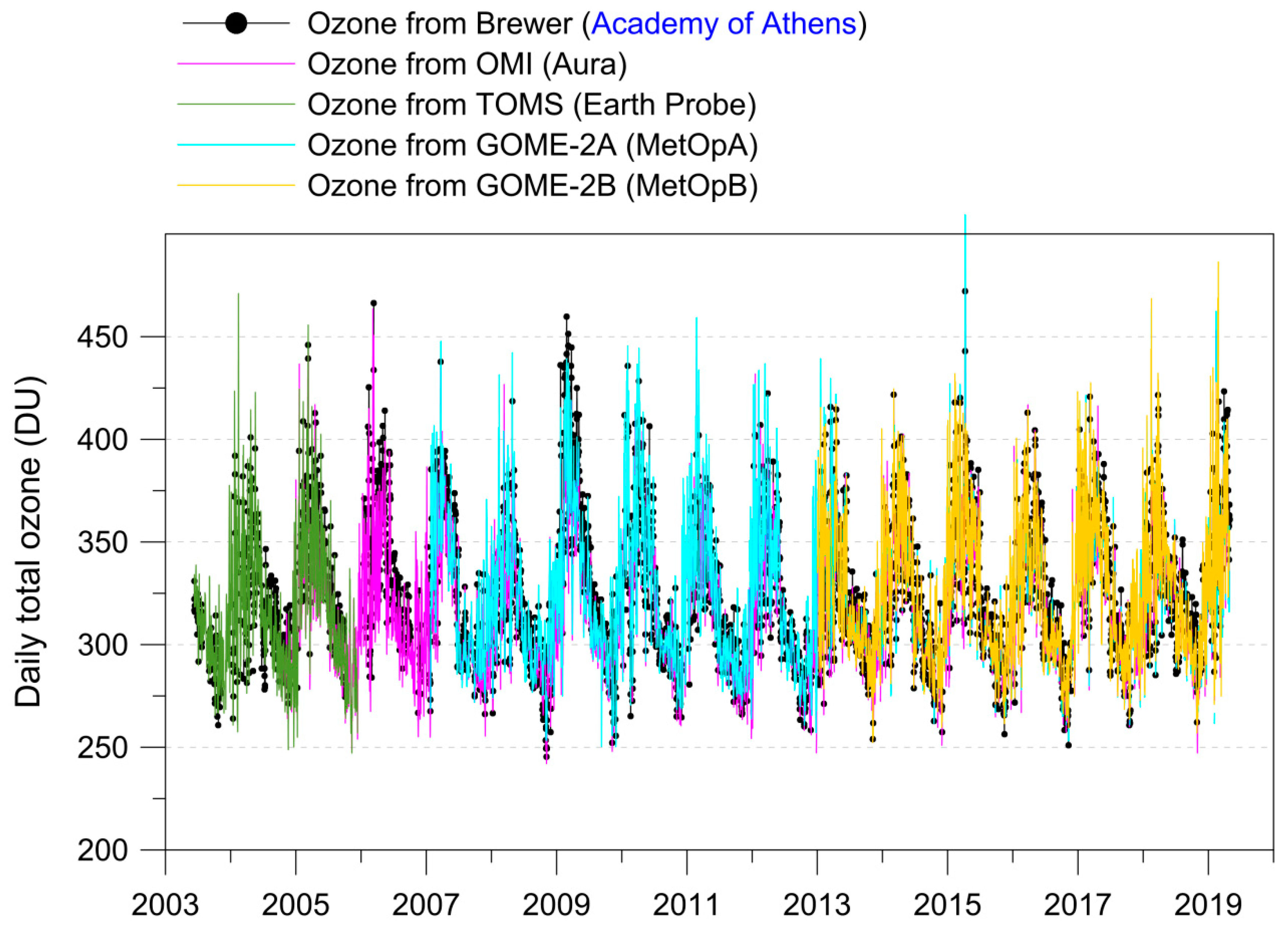
The daily column ozone measurements made by the Brewer spectrophotometer at the Academy of Athens from July 2003 to July 2019 are presented in Figure 1. The respective ozone columns retrieved by TOMS, OMI, GOME-2A, and GOME-2B satellite instruments agree fairly well with the ground-based Brewer measurements. The satellite overpass data were selected to be within a 100 km radius from the Brewer site. The daily values span between 250 DU and 500 DU; in full agreement with Tzanis [26], who compared daily column ozone observations from the Dobson spectrophotometer with SCIAMACHY, TOMS, and OMI satellite data. A good agreement between satellite data and a Brewer spectrophotometer has been demonstrated in other studies, for instance in Kim et al. [27], who used a Brewer spectrophotometer to evaluate the quality of the total ozone column (TOC) produced by multiple polar-orbit satellite measurements at three stations in Antarctica. As a result of their study, high correlations between the TOC from the Brewer and the TOC from TROPOMI and OMI measurements were observed, contrary to the correlations from AIRS measurements. The study confirmed the high quality of OMI TOCs.
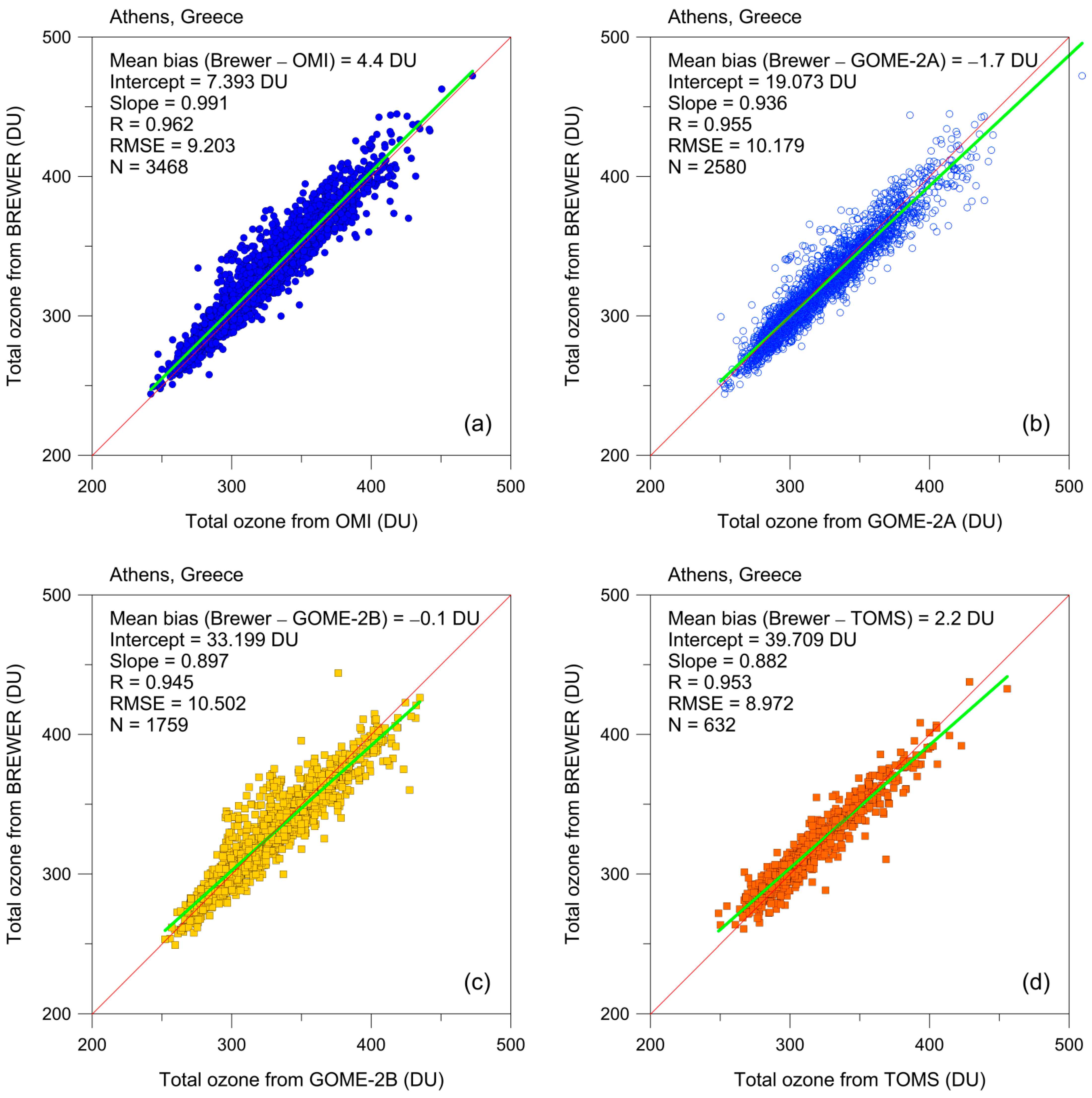
Figure 2 presents the Pearson correlation coefficients, R, the mean biases, the linear fit coefficients, and the root mean square error (RMSE) between ozone from the Brewer spectrophotometer and ozone from each of the satellite instruments. The numbers speak for themselves. The R between the Brewer and OMI, GOME-2A, GOME-2B, and TOMS ozone data are 0.962, 0.955, 0.945, and 0.953, respectively. The mean biases and RMSE between the four data pairs are: 4.4 DU and 9.2 DU (Brewer vs. OMI), −1.7 DU and 10.2 DU (Brewer vs. GOME-2A), −0.1 DU and 10.5 DU (Brewer vs. GOME-2B), and 2.2 DU and 9.0 DU (Brewer vs. TOMS). Accordingly, we provide the mean biases and RMSE between the four satellite data pairs of OMI, TOMS, GOME-2A, and GOME-2B, as follows: −5.3 DU and 7.8 DU (OMI vs. GOME-2A), −4.8 DU and 7.6 DU (OMI vs. GOME-2B), −2.7 DU and 7.7 DU (OMI vs. TOMS), and −1.5 DU and 5.2 DU (GOME-2A vs. GOME-2B). All R were tested for significance using the t–test formula for the correlation coefficient with n − 2 degrees of freedom [28] and were found to be statistically significant at a confidence level greater than 99%. More detailed correlation statistics between the various data pairs are provided in Table 1. It is evident that all correlation coefficients pass the significance level (p-values < 0.0001). We include here for the reader the statistical test of the correlation coefficient, which is:
3.2. Monthly Means and Annual Cycle
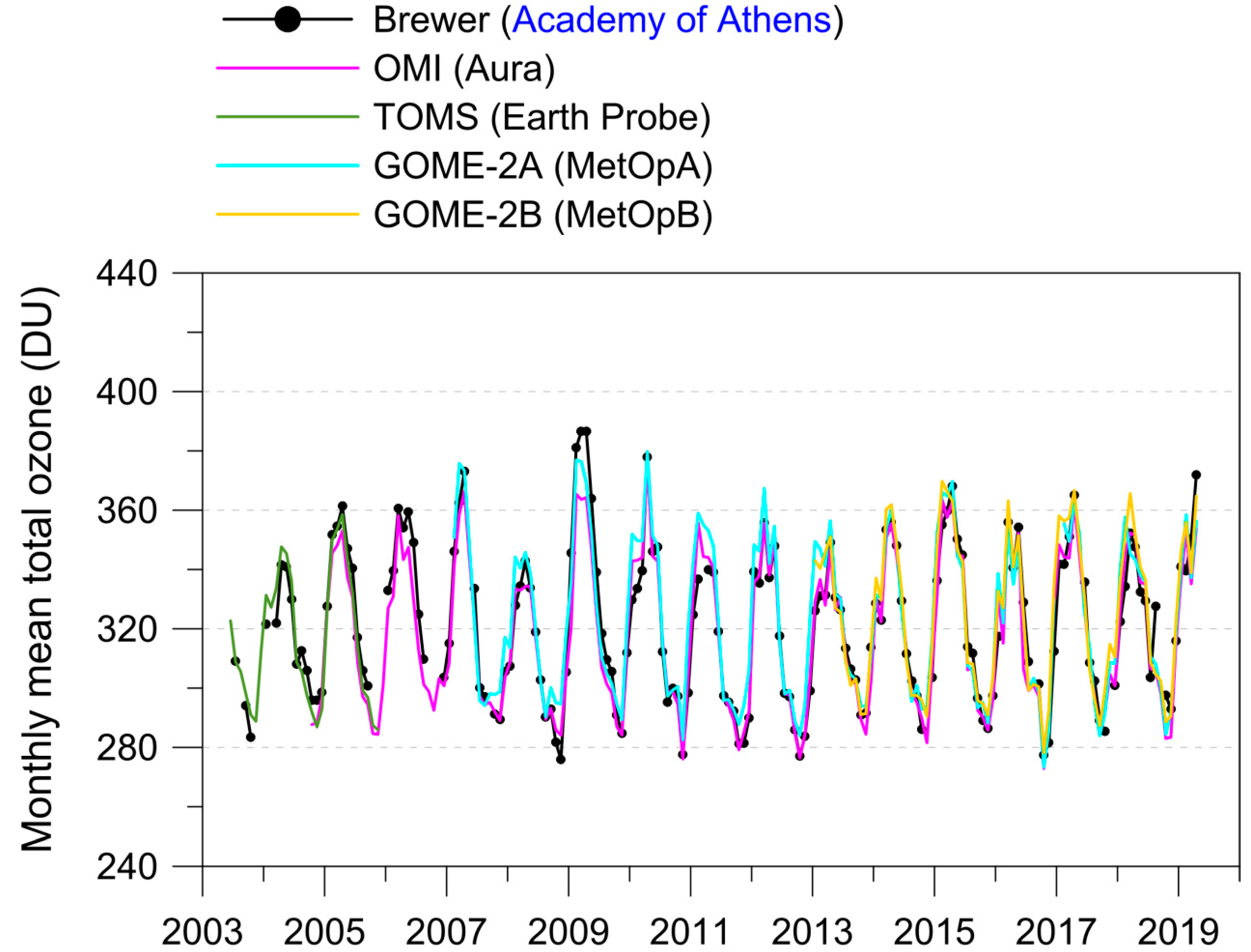
The monthly mean total ozone time series were computed from at least 14 daily averages and are shown in Figure 3 for the Brewer ground-based data in comparison to OMI, TOMS, GOME-2A, and GOME-2B satellite data. The monthly mean values range between 270 DU and 400 DU; again in agreement with results from Tzanis [18]. The long term mean ±2σ of total ozone over Athens is estimated to be 322 ± 53 DU, with no significant change since 2003. The respective estimates from OMI, TOMS, GOME-2A, and GOME-2B satellite data are 318 ± 51 DU, 316 ± 46 DU, 324 ± 53 DU, and 325 ± 51 DU, accordingly.
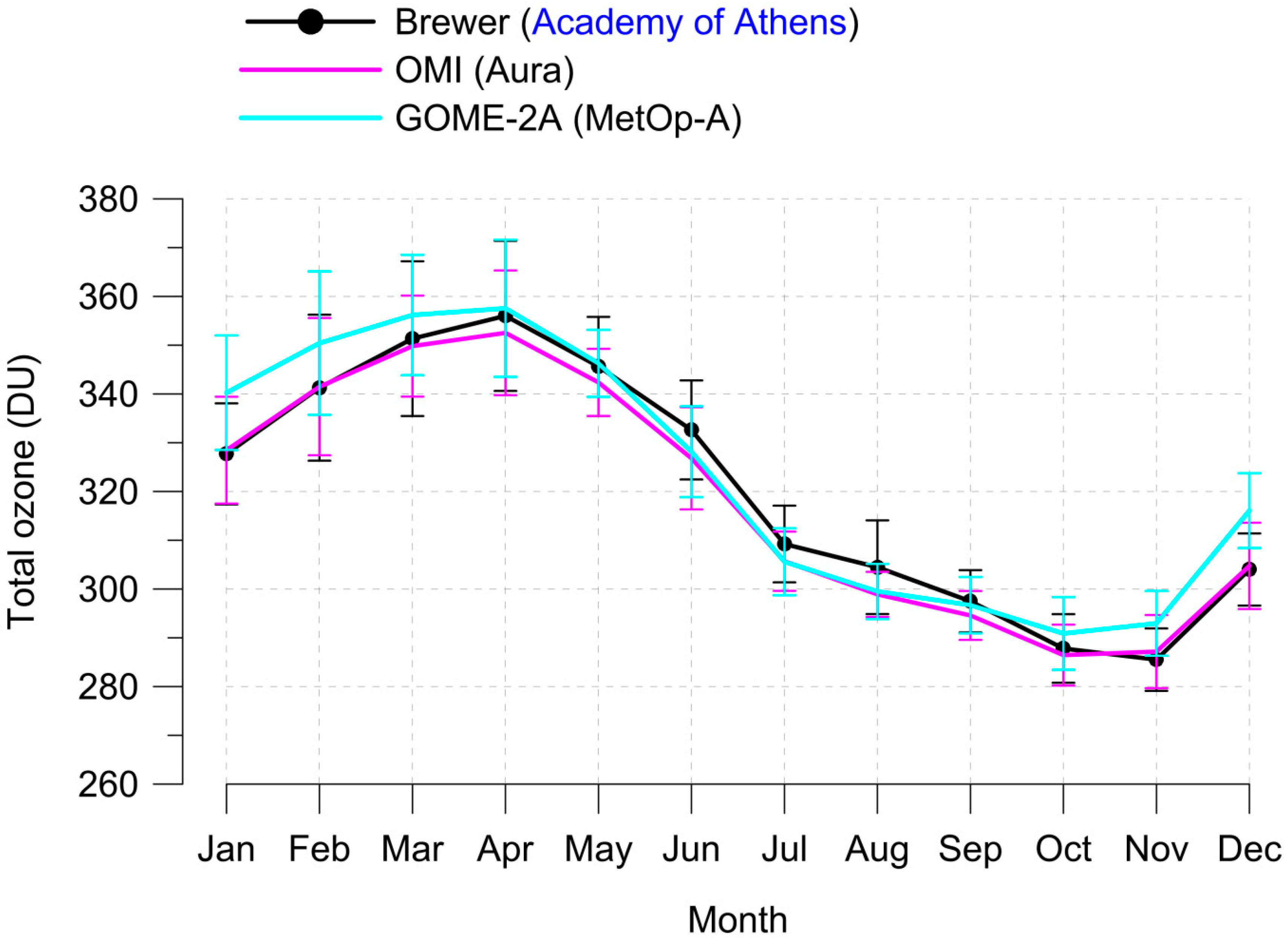
Figure 4 shows the seasonal cycle of total ozone over Athens for the period 2004–2018 from Brewer ground-based measurements and OMI and GOME-2A satellite retrievals. The highest values occurred in spring in March and April, while the lowest values occurred in autumn in October and November. This is a general and consistent feature seen in all three datasets. The explanation for the observed seasonal cycle is transport mechanisms. The spring maximums are a result of the increased transport of ozone from its source region in the tropics toward high latitudes during late autumn and winter. This poleward ozone transport is much weaker during the summer and early autumn periods and is weaker overall in the Southern Hemisphere [2]. Ozone transport from the tropics to the poles is caused by stratospheric wind patterns. In the mid-latitudes these patterns, known as the Brewer–Dobson circulation, make the ozone layer thickest in the spring and thinnest in the fall.
Table 2 summarizes the monthly mean differences between the Brewer, OMI, and GOME-2A total ozone data. The Brewer–OMI differences are within ±1% in all months except June, July, and August, where they are within ±2%, but even these are considered small. We note here that a difference of 1% corresponds to about 3 DU. Differences larger than ±2% are found between Brewer and GOME-2A in the winter months (November, December, January, and February). Similar deviations, larger than 2%, are also found between GOME-2A and OMI satellite data.
With regard to the observed differences, we must keep in mind that the Brewer instrument is operating at ground level, while the satellite instruments are measuring from space using different retrieval algorithms than the ground based instrument. The Brewer instrument is measuring continuously the ozone amount overhead, while the satellite instruments provide few measurements during the day, sometimes one or two measurements. In addition, the Brewer is a remote sensing instrument, while for the satellite data, we processed measurements within a 100 km radius from the Brewer site. The aforementioned issues are known to cause differences between ground measurements and satellite overpasses. However, despite the different approaches of the ground and satellite instruments, the average long-term differences between the ground and satellite measurements are small, within ±1%, indicating the maturity of the measuring systems in achieving such small deviations in the long-term.
3.3. Ozone Variability
We estimated the contribution of different explanatory variables to ozone fluctuations using MLR analysis, as explained in Section 2. The MLR statistical model is of the following form:
where i denotes the month and j is the year of the deseasonalized total ozone column (desTOC) and its components; that is, the QBO at 30 and 50 hPa, the ENSO, the NAO, the solar cycle effect (SOLAR), a straight line to fit the long term trend (TREND), and finally a tropopause pressure related term (TROP). We remind here that TOC data were deseasonalized by subtracting the long-term monthly mean (2004–2018) pertaining to the same calendar month. The contribution of the individual proxy terms is shown in Figure 5. The MLR analysis was applied to the deseasonalized ozone data, which are shown on the top panel of Figure 5 (black line). The two terms representing the QBO are shown by the lines with blue colors, followed by the ENSO term (red line), the NAO term (green line), the solar cycle term (orange line), and the trend term (brown line). The bottom panel of Figure 5 shows the residuals of ozone from the MLR model (grey color), together with the respective residuals of tropopause pressure from an MLR analysis that had been applied to the tropopause data in a previous step (magenta color). The ozone residuals are well correlated with the tropopause pressure residuals, indicating the dynamical influence on ozone induced by the tropopause movement. The graph shows that whenever the tropopause pressure decreases, i.e., tropopause height increases, the amount of ozone increases, and vice versa. We estimate that the correlation coefficient between ozone and tropopause height variations in Athens is +0.448 (slope = 0.376, error = 0.058, t-value = 6.533, p < 0.0001, N = 172).
The MLR regression coefficients and their standard errors are presented in Table 3. It appears that the regression coefficient of the QBO50 proxy is significant at the 90% confidence level (coefficient = 0.111, error = 0.059, t-value = 1.874, p-value = 0.063). The regression coefficient of the solar proxy is more significant than the QBO50 proxy (coefficient = −0.070, error = 0.018, t-value = −3.853, p-value = 0.00017). The regression coefficient of the trend proxy is not statistically significant (coefficient = 0.003, error = 0.013, t-value = 0.249, p-value = 0.803). Finally, the regression coefficient of the tropopause proxy is 0.378 ± 0.059 (t-value = 6.459, p-value < 0.0001).
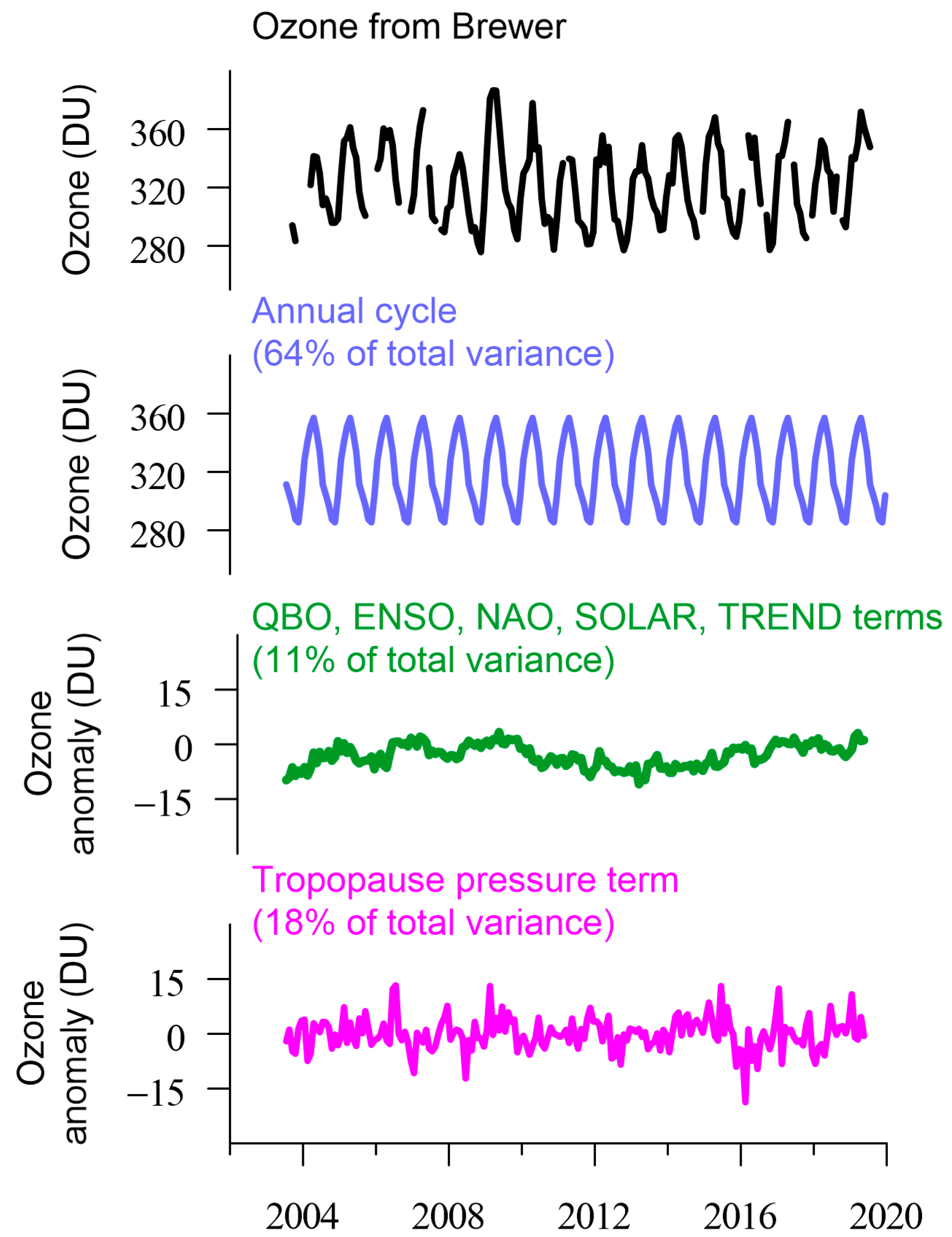
Figure 6 summarizes the monthly ozone data from the Brewer spectrophotometer, the seasonal cycle, the QBO (30 hPa, 50 hPa), ENSO, NAO, solar cycle and trend components joined together, and an estimated tropopause pressure related component. The amplitude of the annual cycle, calculated as ((maximum value–minimum value)/2), is about 35 DU and is estimated to contribute to about 64% to the observed ozone fluctuations. The QBO, ENSO, NAO, SOLAR, and TREND terms are estimated to together explain about 11% of the observed ozone fluctuations. Adding a tropopause pressure related term, the statistical model explains about 27% of ozone fluctuations.
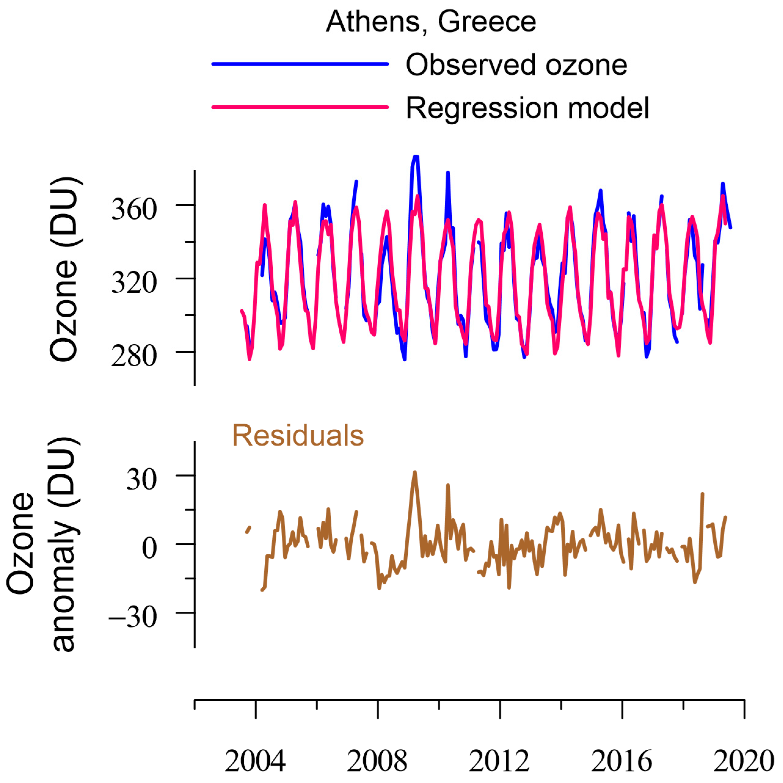
The contribution of all components to ozone fluctuations cumulatively is presented in Figure 7, which shows the observed versus the regressed ozone data. As can be seen, there is good agreement between the observed ozone data and the statistical model calculations obtained from Equation (7). The correlation coefficient between the observed and regressed ozone data is estimated as R = +0.941. The residuals (observed minus regressed data) are shown in the bottom panel.
4. Conclusions
We analyzed 16 years of total ozone measurements over Athens, Greece, with a Brewer spectrophotometer. The main findings can be summarized as follows:
- There are strong correlations between total ozone from the Brewer spectrophotometer and total ozone from the OMI, TOMS, GOME-2A and GOME-2B satellite instruments greater than 0.9.
- The main contribution to ozone variability comes from the seasonal cycle. We estimate that the seasonal variability explains about 64% of the variability in total ozone over Athens.
- Natural fluctuations (QBO, ENSO, NAO, solar cycle trend) together explain about 11% of total ozone variability. Adding the variability related to the tropopause pressure, the multiple linear regression model explains about 27% of ozone fluctuations.
- Accounting for seasonal, solar cycle, and tropopause pressure variability in a statistical regression model, we can simulate the variability of total ozone over Athens quite well.
- We estimate a small, insignificant change in total ozone over Athens, Greece, during the period 2003–2019 of 0.6 ± 4.9 DU (change ±2 standard error limits).
Supplementary Materials
The following are available online at https://0-www-mdpi-com.brum.beds.ac.uk/article/10.3390/oxygen1010005/s1, Figure S1: Information about the stability of the Brewer spectrophotometer according to the calibrations of the instrument in (1) 2004, (2) 2007, (3) 2010, (4) 2013 and (5) 2019.
Author Contributions
Conceptualization, K.E.; methodology, K.E., C.Z.; software, K.E.; formal analysis, K.E.; investigation, K.E., D.K., C.Z.; data curation, K.E., D.K.; writing—original draft preparation, K.E., D.K.; writing—review and editing, K.E., D.K.; visualization, K.E.; supervision, C.Z.; project administration, K.E., D.K.; funding acquisition, K.E., C.Z. All authors have read and agreed to the published version of the manuscript.
Funding
This research was partially funded by the Hellenic Foundation for Research and Innovation (H.F.R.I.) under the “First Call for H.F.R.I. Research Projects to support Faculty members and Researchers and the procurement of high-cost research equipment grant” (Project Number: 300).
Institutional Review Board Statement
Not applicable.
Informed Consent Statement
Not applicable.
Data Availability Statement
Brewer ozone data are submitted to WOUDC (Station ID 449-Academy of Athens) (https://woudc.org/data/stations/) (accessed on 25 June 2021). OMI and GOME-2 satellite ozone data were downloaded from the NASA Aura Validation Data Center (https://avdc.gsfc.nasa.gov/index.php?site=599065317) (access on 8 May 2021). The QBO data were provided by FU-Berlin (http://www.geo.fu-berlin.de/met/ag/strat/produkte/qbo/qbo.dat) (last access: 8 May 2021). The SOI data were provided from the Bureau of Meteorology of the Australian Government (http://www.bom.gov.au/climate/current/soi2.shtml) (access on 8 May 2021). The sunspots numbers were provided from the WDC Sunspot Index and Long-term Solar Observations of the Royal Observatory of Belgium, Brussels (http://sidc.be/silso/datafiles) (access on 8 May 2021). The NAO index was provided from NCAR Climate Data Guide (https://climatedataguide.ucar.edu/climate-data/hurrell-north-atlantic-oscillation-nao-index-pc-based) (access on 8 May 2021).
Acknowledgments
We the acknowledge support and funding of this work by the project “Panhellenic Infrastructure for Atmospheric Composition and Climate Change” (MIS 5021516), which is implemented under the action “Reinforcement of the Research and Innovation Infrastructure”, funded by the Operational Program “Competitiveness, Entrepreneurship and Innovation” (NSRF 2014–2020) and co-financed by Greece and the European Union (European Regional Development Fund).
Conflicts of Interest
The authors declare no conflict of interest.
References
- Langematz, U. Stratospheric ozone: Down and up through the anthropocene. ChemTexts 2019, 5, 8. [Google Scholar] [CrossRef] [Green Version]
- Salawitch, R.J.; Fahey, D.W.; Hegglin, M.I.; McBride, L.A.; Tribett, W.R.; Doherty, S.J. Twenty Questions and Answers About the Ozone Layer: 2018 Update, Scientific Assessment of Ozone Depletion: 2018; World Meteorological Organization: Geneva, Switzerland, 2019; p. 84. [Google Scholar]
- Bais, A.F.; Bernhard, G.; McKenzie, R.L.; Aucamp, P.J.; Young, P.J.; Ilyas, M.; Jöckel, P.; Deushi, M. Ozone–climate interactions and effects on solar ultraviolet radiation. Photochem. Photobiol. Sci. 2019, 18, 602–640. [Google Scholar] [CrossRef] [PubMed] [Green Version]
- Bais, A.F.; McKenzie, R.L.; Bernhard, G.; Aucamp, P.J.; Ilyas, M.; Madronich, S.; Tourpali, K. Ozone depletion and climate change: Impacts on UV radiation. Photochem. Photobiol. Sci. 2014, 14, 19–52. [Google Scholar] [CrossRef] [PubMed]
- Varotsos, C.A.; Cracknell, A.P. Three years of total ozone measurements over Athens obtained using the remote sensing technique of a Dobson spectrophotometer. Int. J. Remote Sens. 1994, 15, 1519–1524. [Google Scholar] [CrossRef]
- Varotsos, C.A. Total ozone measurements over Athens: Intercomparison between Dobson, TOMS (version 6) and SBUV measurements. Int. J. Remote Sens. 1998, 19, 3327–3333. [Google Scholar] [CrossRef]
- Fragkos, K.; Taylor, M.; Bais, A.F.; Fountoulakis, I.; Tourpali, K.; Meleti, C.; Zempila, M.M. Multi-decadal Trend Analysis of Total Columnar Ozone Over Thessaloniki. In Perspectives on Atmospheric Sciences; Karacostas, T.S., Bais, A.F., Nastos, P.T., Eds.; Springer Atmospheric Sciences, Springer International Publishing: Cham, Switzerland, 2017; pp. 983–988. [Google Scholar] [CrossRef]
- World Meteorological Organization. Scientific Assessment of Ozone Depletion: 2010; Report No. 52; Global Ozone Research and Monitoring Project: Geneva, Switzerland, 2011; p. 516. [Google Scholar]
- Zerefos Lab. Available online: http://www.bioacademy.gr/lab/zerefos (accessed on 25 June 2021).
- Gerasopoulos, E.; Kokkalis, P.; Amiridis, V.; Liakakou, E.; Perez, C.; Haustein, K.; Eleftheratos, K.; Andreae, M.; Andreae, T.W.; Zerefos, C.S.; et al. Dust specific extinction cross-sections over the Eastern Mediterranean using the BSC-DREAM model and sun photometer data: The case of urban environments. Ann. Geophys. 2009, 27, 2903–2912. [Google Scholar] [CrossRef] [Green Version]
- Kerr, J.B.; McElroy, C.T.; Olafson, R.A. Measurements of ozone with the Brewer ozone spectrophotometer. In Proceedings of the Quadrennial Ozone Symposium, Boulder, CO, USA, 4–9 August 1981; London, J., Ed.; National Center for Atmospheric Research: Boulder, CO, USA, 1980; pp. 74–79. [Google Scholar]
- Kerr, J.B. The Brewer Spectrophotometer. In UV Radiation in Global Climate Change; Gao, W., Schmoldt, D.L., Slusser, J.R., Eds.; Springer: Berlin/Heidelberg, Germany, 2010; pp. 160–191. [Google Scholar] [CrossRef]
- Software for Ozone Spectrophotometers. Available online: http://www.o3soft.eu/o3brewer.html (accessed on 30 April 2021).
- Kazantzidis, A.; Bais, A.F.; Zempila, M.M.; Meleti, C.; Eleftheratos, K.; Zerefos, C.S. Evaluation of ozone column measurements over Greece with NILU-UV multi-channel radiometers. Int. J. Remote Sens. 2009, 30, 4273–4281. [Google Scholar] [CrossRef]
- Raptis, P.I.; Kazadzis, S.; Eleftheratos, K.; Kosmopoulos, P.; Amiridis, V.; Helmis, C.; Zerefos, C. Total ozone column measurements using an ultraviolet multi-filter radiometer. Int. J. Remote Sens. 2015, 36, 4469–4482. [Google Scholar] [CrossRef]
- Fioletov, V.E.; Kerr, J.B.; Wardle, D.I.; Wu, E. Correction of stray light for the Brewer single monochromator. In Atmospheric Ozone, Proceedings of the Quadrennial Ozone Symposium, Hokkaido University, Sapporo, Japan, 3–8 July 2000; Shibasaki, K., Bojkov, R.D., Eds.; Hokkaido University: Sapporo, Japan, 2000; pp. 371–372. [Google Scholar]
- Weatherhead, E.; Theisen, D.; Stevermer, A.; Enagonio, J.; Rabinovitch, B.; Disterhoft, P.; Lantz, K.; Meltzer, R.; DeLuisi, J.; Rives, J.; et al. Temperature dependence of the Brewer ultraviolet data. J. Geophys. Res. Space Phys. 2001, 106, 34121–34129. [Google Scholar] [CrossRef]
- Zanjani, Z.V.; Moeini, O.; McElroy, T.; Barton, D.; Savastiouk, V. A calibration procedure which accounts for non-linearity in single-monochromator Brewer ozone spectrophotometer measurements. Atmos. Meas. Tech. 2019, 12, 271–279. [Google Scholar] [CrossRef] [Green Version]
- Naujokat, B. An Update of the Observed Quasi-Biennial Oscillation of the Stratospheric Winds over the Tropics. J. Atmospheric Sci. 1986, 43, 1873–1877. [Google Scholar] [CrossRef] [Green Version]
- Dameris, M.; Nodorp, D.; Sausen, R. Correlation between Tropopause Height Pressure and TOMS-Data for the EASOE-Winter 1991/1992. Beitr. Phys. Atmos. 1995, 68, 227–232. [Google Scholar]
- Hoinka, K.P.; Claude, H.; Köhler, U. On the correlation between tropopause pressure and ozone above central Europe. Geophys. Res. Lett. 1996, 23, 1753–1756. [Google Scholar] [CrossRef]
- Steinbrecht, W.; Claude, H.; Köhler, U.; Hoinka, K.P. Correlations between tropopause height and total ozone: Implications for long-term changes. J. Geophys. Res. Space Phys. 1998, 103, 19183–19192. [Google Scholar] [CrossRef]
- Kalnay, E.; Kanamitsu, M.; Kistler, R.; Collins, W.; Deaven, D.; Gandin, L.; Iredell, M.; Saha, S.; White, G.; Woollen, J.; et al. The NCEP/NCAR 40-year reanalysis project. Bull. Am. Meteorol. Soc. 1996, 77, 437–472. [Google Scholar] [CrossRef] [Green Version]
- Zerefos, C.; Kapsomenakis, J.; Eleftheratos, K.; Tourpali, K.; Petropavlovskikh, I.; Hubert, D.; Godin-Beekmann, S.; Steinbrecht, W.; Frith, S.; Sofieva, V.; et al. Representativeness of single lidar stations for zonally averaged ozone profiles, their trends and attribution to proxies. Atmos. Chem. Phys. Discuss. 2018, 18, 6427–6440. [Google Scholar] [CrossRef] [Green Version]
- Eleftheratos, K.; Kapsomenakis, J.; Zerefos, C.S.; Bais, A.F.; Fountoulakis, I.; Dameris, M.; Jöckel, P.; Haslerud, A.S.; Godin-Beekmann, S.; Steinbrecht, W.; et al. Possible Effects of Greenhouse Gases to Ozone Profiles and DNA Active UV-B Irradiance at Ground Level. Atmosphere 2020, 11, 228. [Google Scholar] [CrossRef] [Green Version]
- Tzanis, C. Total ozone observations at Athens, Greece by satellite-borne and ground-based instrumentation. Int. J. Remote Sens. 2009, 30, 6023–6033. [Google Scholar] [CrossRef]
- Kim, S.; Park, S.-J.; Lee, H.; Ahn, D.; Jung, Y.; Choi, T.; Lee, B.; Kim, S.-J.; Koo, J.-H. Evaluation of Total Ozone Column from Multiple Satellite Measurements in the Antarctic Using the Brewer Spectrophotometer. Remote Sens. 2021, 13, 1594. [Google Scholar] [CrossRef]
- von Storch, H.; Zwiers, F.W. Statistical Analysis in Climate Research; Cambridge University Press: Cambridge, UK, 1999; 484p, ISBN 0521450713. [Google Scholar]
Figure 1.
Daily total ozone over Athens, Greece (2003–2019) from Brewer ground-based measurements and OMI, TOMS, and GOME-2A and GOME-2B satellite measurements.
Figure 1.
Daily total ozone over Athens, Greece (2003–2019) from Brewer ground-based measurements and OMI, TOMS, and GOME-2A and GOME-2B satellite measurements.

Figure 2.
Correlation analysis between the Brewer and satellite ozone measurements for common days: (a) Brewer and OMI; (b) Brewer and GOME-2A; (c) Brewer and GOME-2B; (d) Brewer and TOMS.
Figure 2.
Correlation analysis between the Brewer and satellite ozone measurements for common days: (a) Brewer and OMI; (b) Brewer and GOME-2A; (c) Brewer and GOME-2B; (d) Brewer and TOMS.

Figure 3.
Monthly mean total ozone from July 2003 to July 2019 calculated from at least 14 daily averages from Brewer ground-based data, and OMI, TOMS, GOME-2A, and GOME-2B satellite data.
Figure 3.
Monthly mean total ozone from July 2003 to July 2019 calculated from at least 14 daily averages from Brewer ground-based data, and OMI, TOMS, GOME-2A, and GOME-2B satellite data.

Figure 4.
Mean annual cycle of total ozone over Athens, Greece (2004–2018) from Brewer ground-based data, and OMI, GOME-2A satellite data.
Figure 4.
Mean annual cycle of total ozone over Athens, Greece (2004–2018) from Brewer ground-based data, and OMI, GOME-2A satellite data.

Figure 5.
Contribution of different explanatory variables to ozone fluctuations over Athens, Greece, obtained from the MLR analysis. The bottom panel shows the residuals of ozone as related to the respective residuals of tropopause pressure.
Figure 5.
Contribution of different explanatory variables to ozone fluctuations over Athens, Greece, obtained from the MLR analysis. The bottom panel shows the residuals of ozone as related to the respective residuals of tropopause pressure.

Figure 6.
Time series of monthly ozone from the Brewer spectrophotometer versus the annual cycle; the QBO, ENSO, NAO, SOLAR, TREND terms grouped together; and the tropopause pressure term separately. The highest contribution comes from the seasonal cycle (see text).
Figure 6.
Time series of monthly ozone from the Brewer spectrophotometer versus the annual cycle; the QBO, ENSO, NAO, SOLAR, TREND terms grouped together; and the tropopause pressure term separately. The highest contribution comes from the seasonal cycle (see text).

Figure 7.
Observed and regressed columnar ozone over Athens, Greece, and respective residuals (observed–regressed).
Figure 7.
Observed and regressed columnar ozone over Athens, Greece, and respective residuals (observed–regressed).


Table 1.
Statistics of correlations between the Brewer and satellite ozone data pairs.
| Data Pair | R | Intercept (DU) | Slope | Error | t-Value | p-Value | RMSE | N |
|---|---|---|---|---|---|---|---|---|
| Brewer vs. OMI | +0.962 | 7.393 | 0.991 | 0.005 | 208.733 | <0.0001 | 9.203 | 3468 |
| Brewer vs. GOME-2A | +0.955 | 19.073 | 0.936 | 0.006 | 163.474 | <0.0001 | 10.179 | 2580 |
| Brewer vs. GOME-2B | +0.945 | 33.199 | 0.897 | 0.007 | 120.840 | <0.0001 | 10.502 | 1759 |
| Brewer vs. TOMS | +0.953 | 39.709 | 0.882 | 0.011 | 79.359 | <0.0001 | 8.972 | 632 |
| OMI vs. GOME-2A | +0.972 | 20.026 | 0.922 | 0.004 | 210.739 | <0.0001 | 7.824 | 2600 |
| OMI vs. GOME-2B | +0.972 | 20.283 | 0.923 | 0.005 | 169.102 | <0.0001 | 7.593 | 1668 |
| OMI vs. TOMS | +0.972 | 25.869 | 0.909 | 0.011 | 83.520 | <0.0001 | 7.736 | 405 |
| GOME-2A vs. GOME-2B | +0.988 | 2.591 | 0.987 | 0.005 | 218.776 | <0.0001 | 5.158 | 1122 |
Table 2.
Mean differences between Brewer and satellite total ozone data (1% ≅ 3 DU).
| Brewer—OMI | Brewer—GOME-2A | GOME-2A—OMI | |
|---|---|---|---|
| January | −0.2% (−1 DU) | −3.7% (−13 DU) | 3.6% (12 DU) |
| February | −0.1% (0 DU) | −2.6% (−9 DU) | 2.6% (9 DU) |
| March | 0.4% (2 DU) | −1.4% (−5 DU) | 1.8% (6 DU) |
| April | 1.0% (3 DU) | −0.4% (−2 DU) | 1.4% (5 DU) |
| May | 1.0% (3 DU) | −0.2% (−1 DU) | 1.1% (4 DU) |
| June | 1.8% (6 DU) | 1.4% (4 DU) | 0.4% (1 DU) |
| July | 1.2% (4 DU) | 1.2% (4 DU) | 0.0% (0 DU) |
| August | 1.9% (6 DU) | 1.7% (5 DU) | 0.2% (1 DU) |
| September | 1.0% (3 DU) | 0.3% (1 DU) | 0.7% (2 DU) |
| October | 0.5% (1 DU) | −1.1% (−3 DU) | 1.5% (4 DU) |
| November | −0.6% (−2 DU) | −2.5% (−7 DU) | 2.0% (6 DU) |
| December | −0.2% (−1 DU) | −3.8% (−12DU) | 3.7% (11 DU) |
| MEAN | 0.6% (2 DU) | −0.9% (−3 DU) | 1.6% (5 DU) |
Table 3.
MLR regression statistics for the proxy terms considered in Equation (7).
| MLR Regression Statistics | Coefficient | Error | t-Value | p-Value |
|---|---|---|---|---|
| Intercept | 2.623 | 1.683 | 1.556 | 0.12102 |
| QBO at 30 hPa | 0.002 | 0.039 | 0.047 | 0.96233 |
| QBO at 50 hPa | 0.111 | 0.059 | 1.874 | 0.06272 |
| ENSO | −0.093 | 0.069 | −1.348 | 0.17953 |
| NAO | 0.678 | 0.632 | 1.073 | 0.28472 |
| SOLAR | −0.070 | 0.018 | −3.853 | 0.00017 |
| TREND | 0.003 | 0.013 | 0.249 | 0.80335 |
| TROPOPAUSE | 0.378 | 0.059 | 6.459 | 1.15 × 10⁹ |
Publisher’s Note: MDPI stays neutral with regard to jurisdictional claims in published maps and institutional affiliations. |
© 2021 by the authors. Licensee MDPI, Basel, Switzerland. This article is an open access article distributed under the terms and conditions of the Creative Commons Attribution (CC BY) license (https://creativecommons.org/licenses/by/4.0/).
Share and Cite
MDPI and ACS Style
Eleftheratos, K.; Kouklaki, D.; Zerefos, C. Sixteen Years of Measurements of Ozone over Athens, Greece with a Brewer Spectrophotometer. Oxygen 2021, 1, 32-45. https://0-doi-org.brum.beds.ac.uk/10.3390/oxygen1010005
AMA Style
Eleftheratos K, Kouklaki D, Zerefos C. Sixteen Years of Measurements of Ozone over Athens, Greece with a Brewer Spectrophotometer. Oxygen. 2021; 1(1):32-45. https://0-doi-org.brum.beds.ac.uk/10.3390/oxygen1010005
Chicago/Turabian StyleEleftheratos, Kostas, Dimitra Kouklaki, and Christos Zerefos. 2021. "Sixteen Years of Measurements of Ozone over Athens, Greece with a Brewer Spectrophotometer" Oxygen 1, no. 1: 32-45. https://0-doi-org.brum.beds.ac.uk/10.3390/oxygen1010005