
Correction of Temperature Variation with Independent Water Samples to Predict Soluble Solids Content of Kiwifruit Juice Using NIR Spectroscopy


Abstract
:1. Introduction
2. Materials and Methods
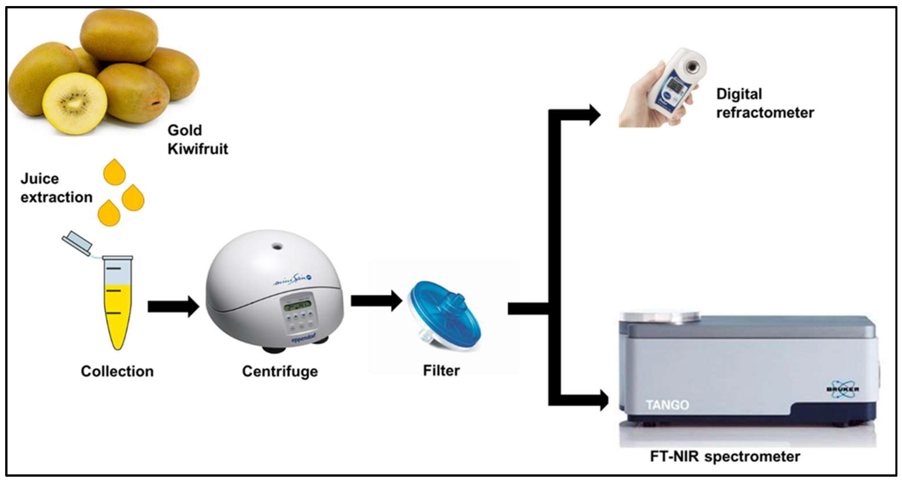
2.1. Sample Preparation
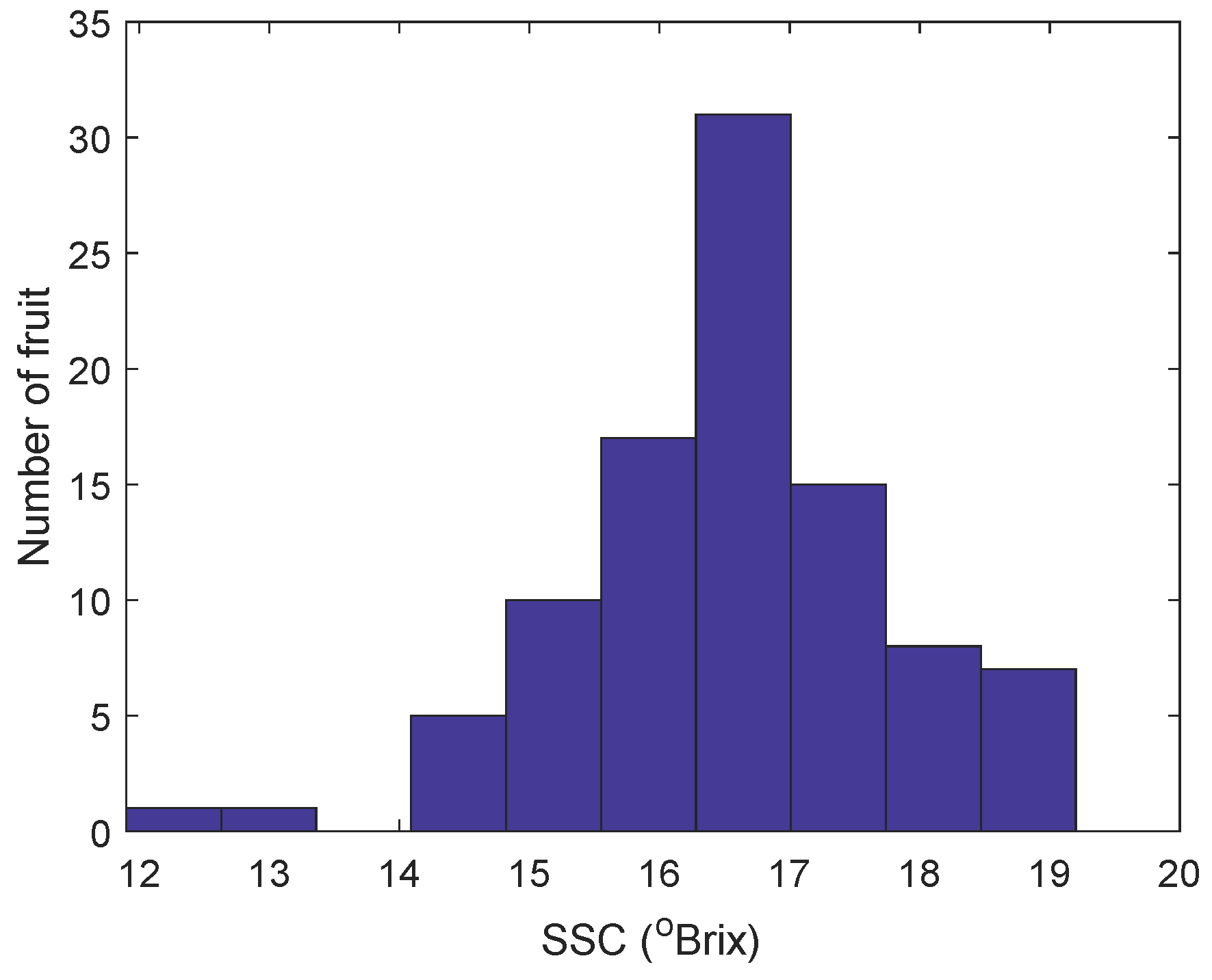
2.2. Reference SSC (°Brix) Measurement
2.3. FT-NIR Spectral Measurements
2.4. Aquaphotomics Analysis
2.5. Multivariate Analysis
2.5.1. SNV + 2D
2.5.2. EMSC
2.5.3. EPO
2.5.4. All Temperature Method
2.6. Statistical Analysis
3. Results and Discussion
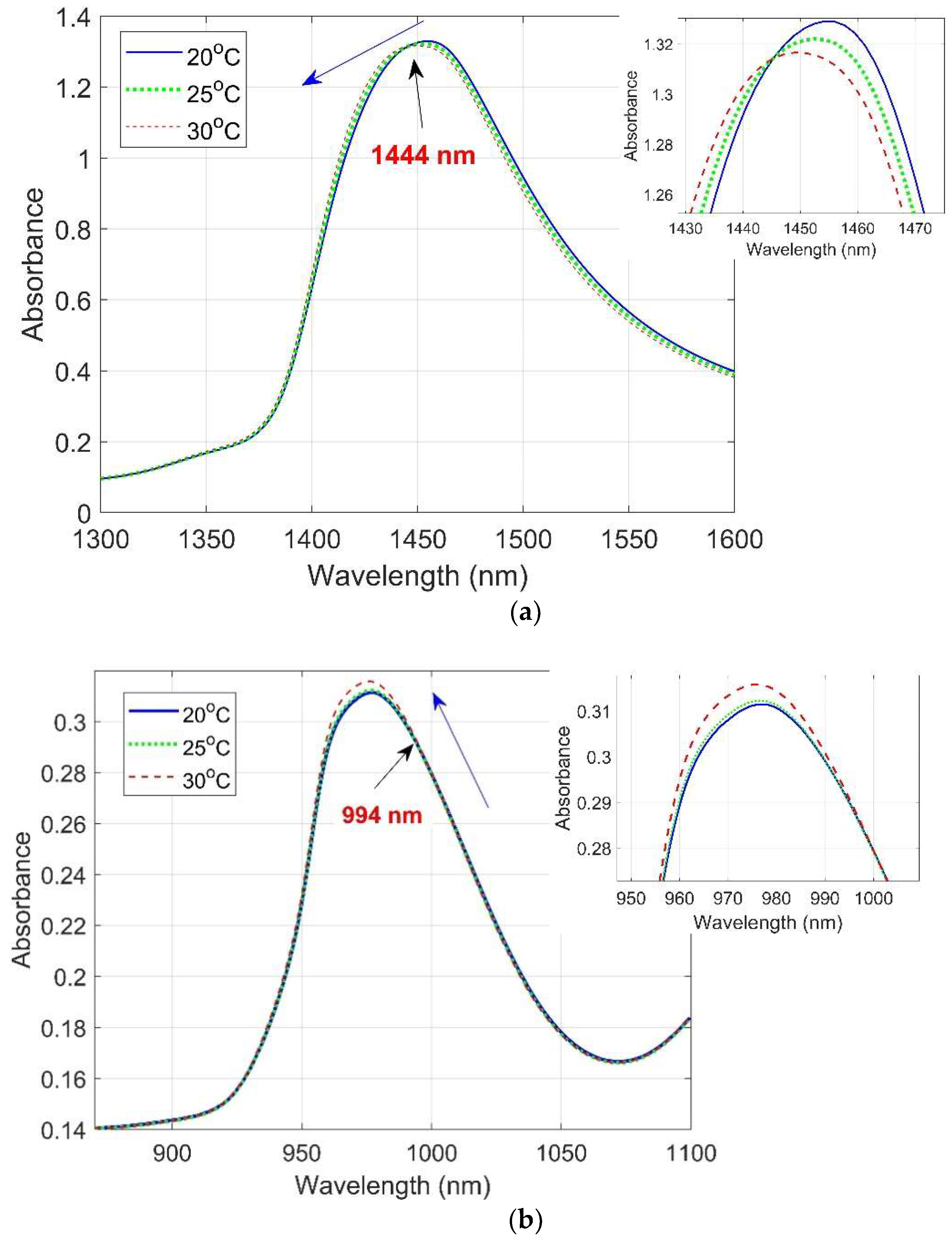
3.1. The Raw Spectra
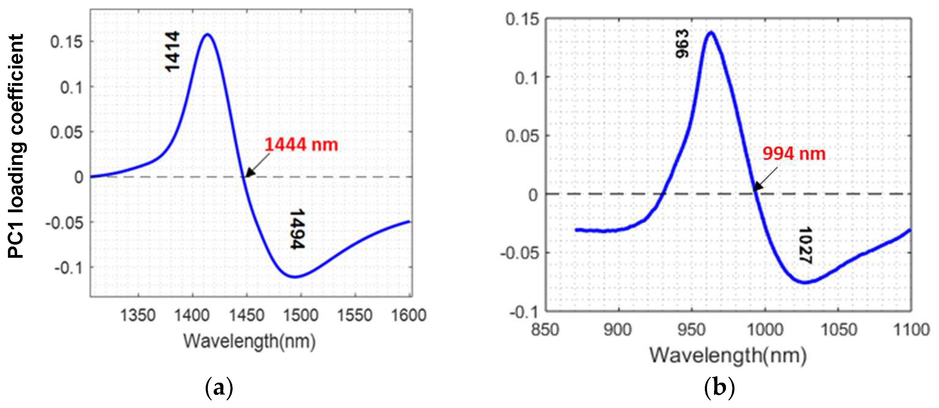
3.2. Aquaphotomics Analysis
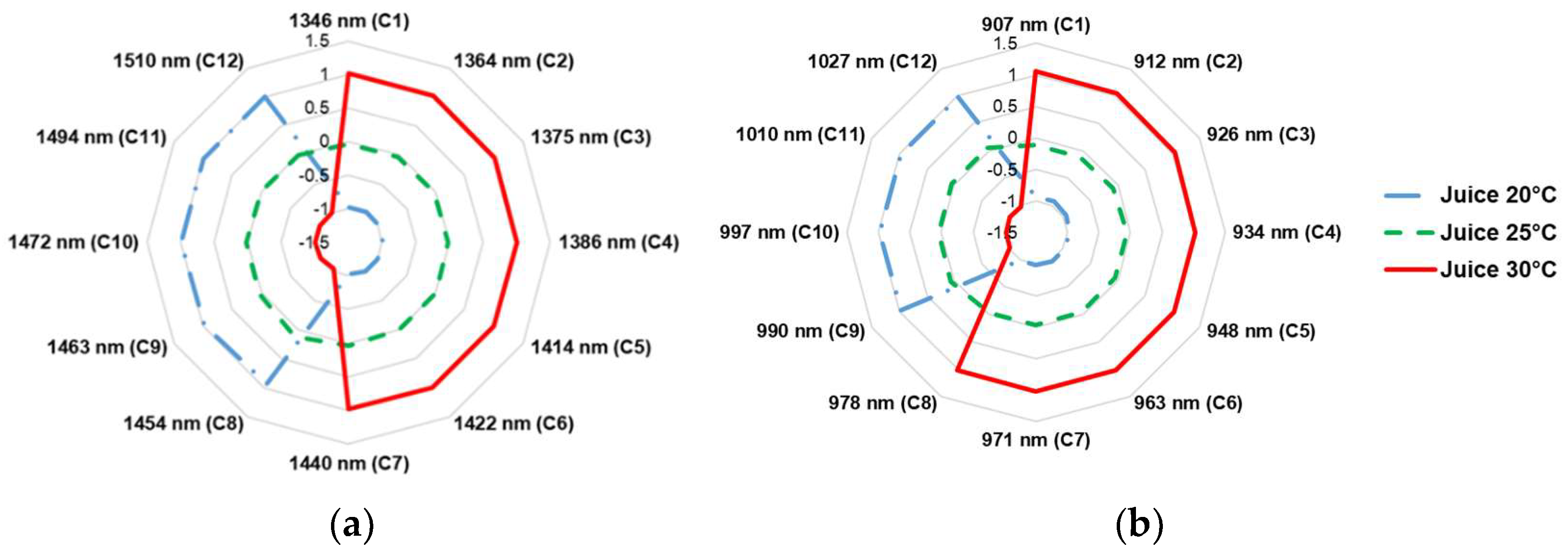
3.3. Aquagrams
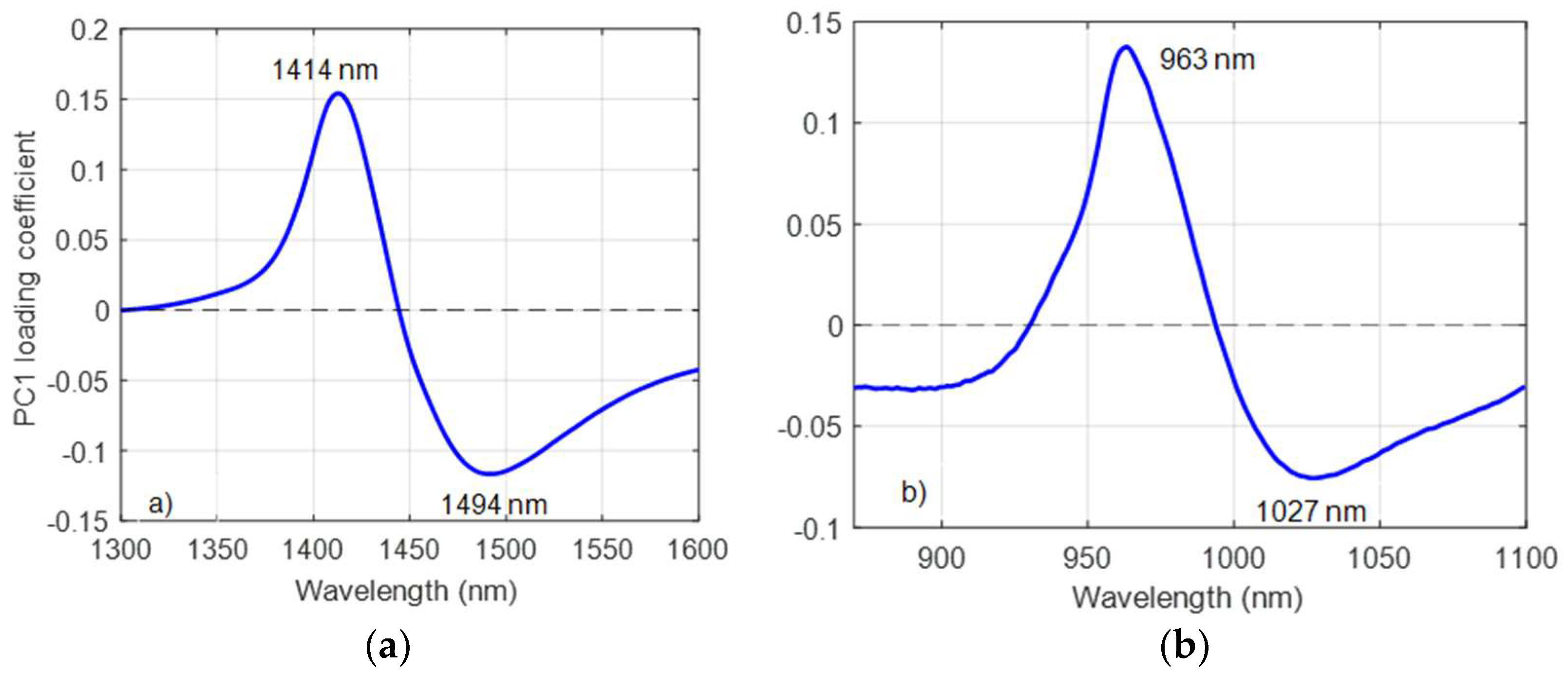
3.4. EMSC Correction
Pure Water Analysis
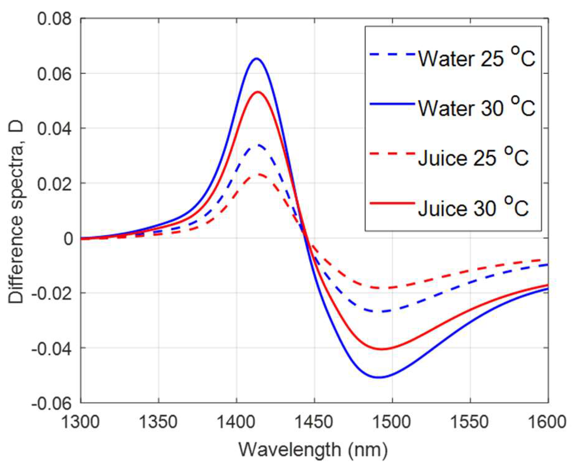
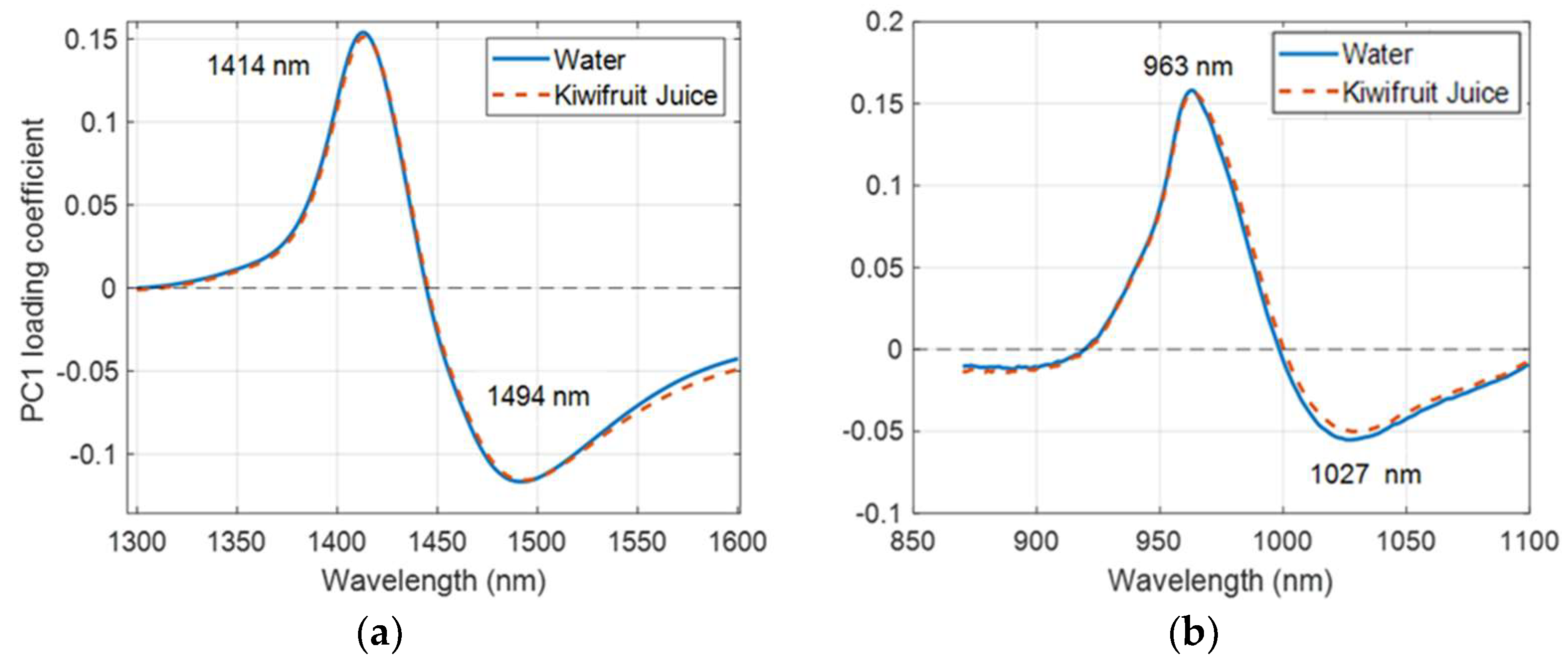
3.5. EPO Correction
PCA of the Difference Matrix D for EPO Correction
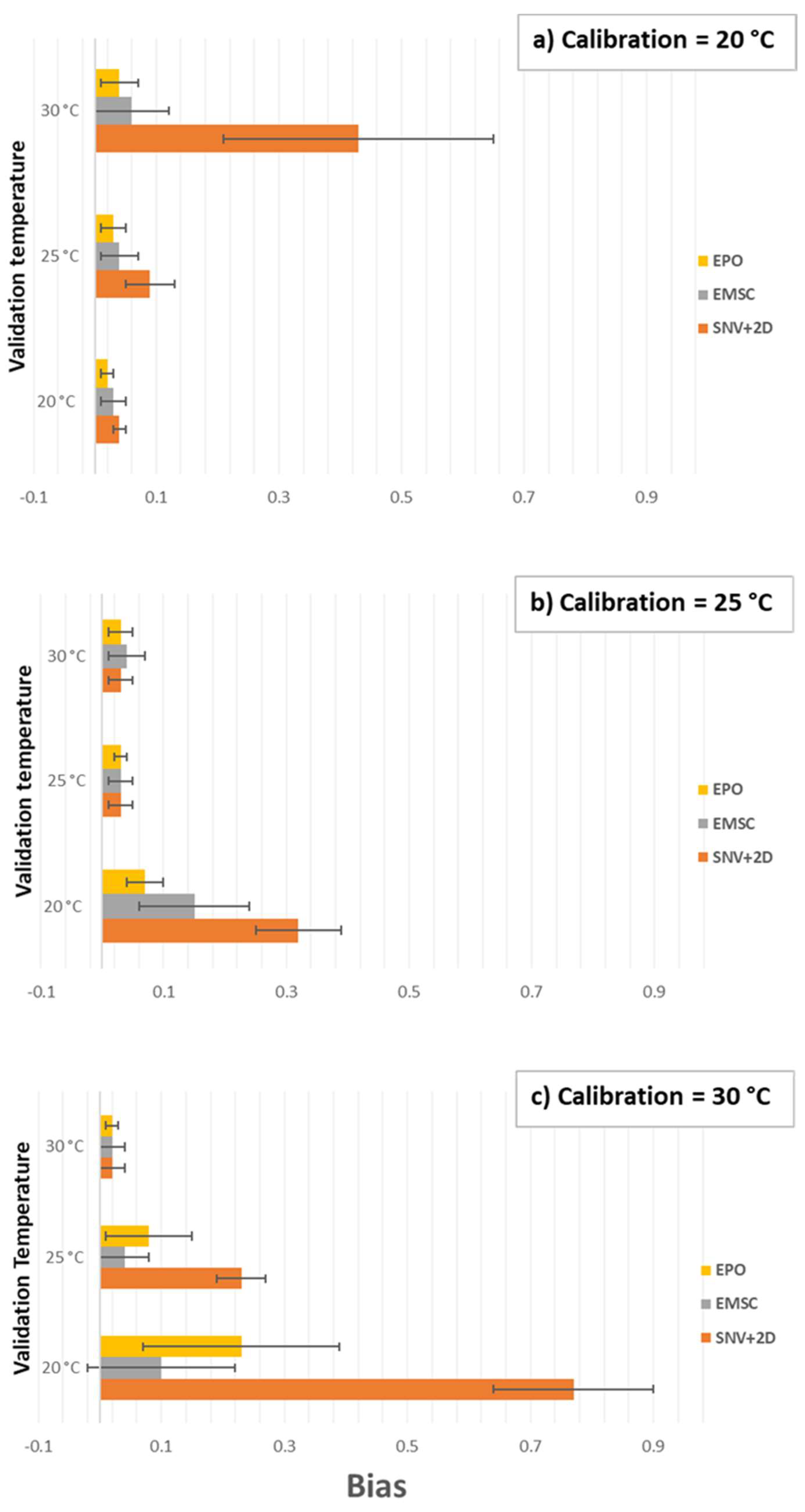
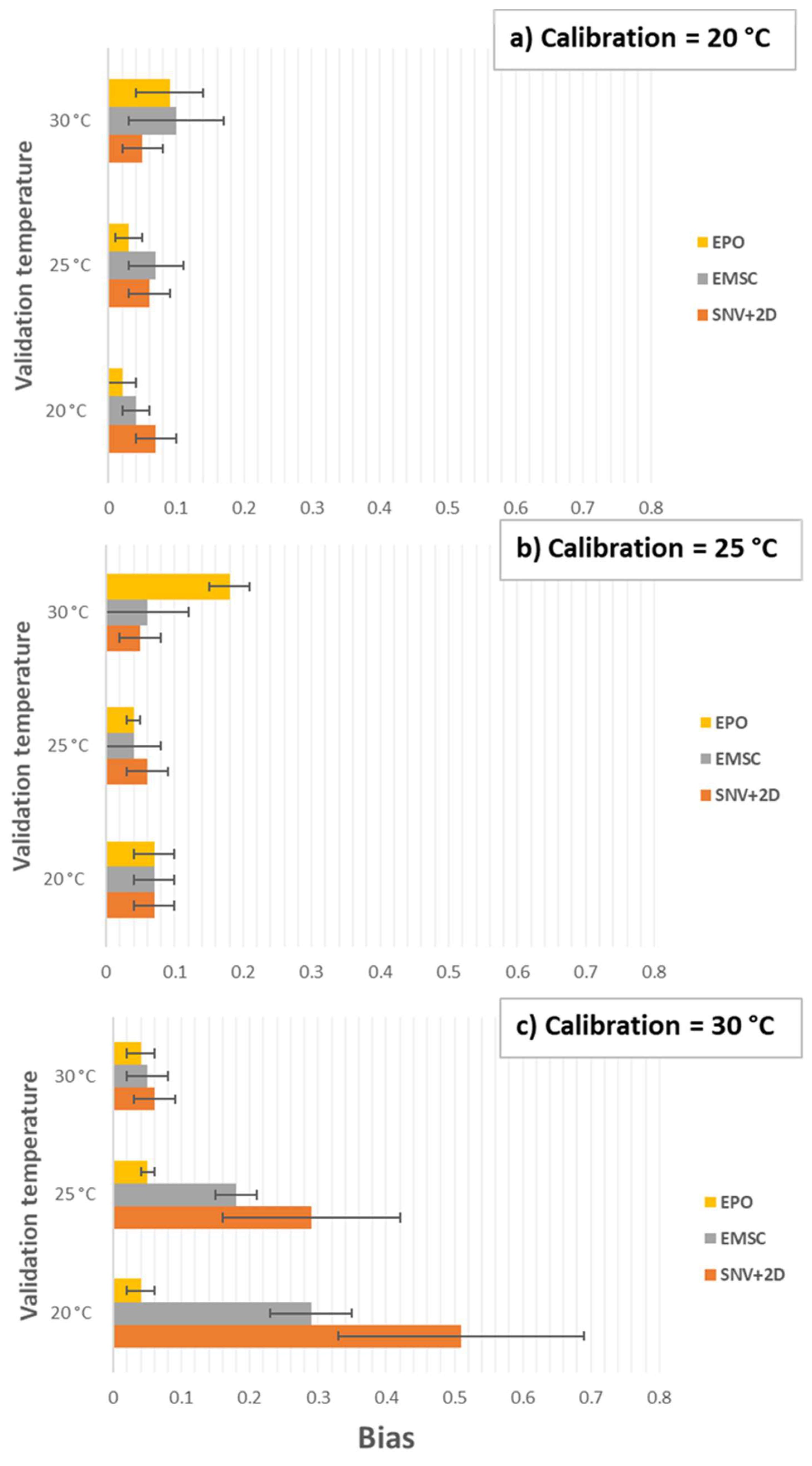
3.6. Prediction of SSC
4. Conclusions
Author Contributions
Funding
Institutional Review Board Statement
Informed Consent Statement
Conflicts of Interest
Sample Availability
References
- Popkin, B.M.; D’Anci, K.E.; Rosenberg, I.H. Water, hydration, and health. Nutr. Rev. 2010, 68, 439–458. [Google Scholar] [CrossRef] [PubMed]
- DeMan, J.M. Water. In Principles of Food Chemistry; Springer: Boston, MA, USA, 1999; pp. 1–32. [Google Scholar]
- Pegau, W.S.; Gray, D.; Zaneveld, J.R.V. Absorption and attenuation of visible and near-infrared light in water: Dependence on temperature and salinity. Appl. Opt. 1997, 36, 6035–6046. [Google Scholar] [CrossRef] [Green Version]
- Tsenkova, R. Aquaphotomics: Water in the biological and aqueous world scrutinised with invisible light. Spectrosc. Eur. 2010, 22, 6–10. [Google Scholar]
- McGlone, V.A.; Jordan, R.B.; Seelye, R.; Clark, C.J. Dry-matter—a better predictor of the post-storage soluble solids in apples? Postharvest Biol. Technol. 2003, 28, 431–435. [Google Scholar] [CrossRef]
- Nicolaï, B.M.; Beullens, K.; Bobelyn, E.; Peirs, A.; Saeys, W.; Theron, K.I.; Lammertyn, J. Nondestructive measurement of fruit and vegetable quality by means of NIR spectroscopy: A review. Postharvest Biol. Technol. 2007, 46, 99–118. [Google Scholar] [CrossRef]
- Wang, Y.; Veltkamp, D.J.; Kowalski, B.R. Multivariate instrument standardization. Anal. Chem. 1991, 63, 2750–2756. [Google Scholar] [CrossRef]
- Segtnan, V.H.; Šašić, Š.; Isaksson, T.; Ozaki, Y. Studies on the Structure of Water Using Two-Dimensional Near-Infrared Correlation Spectroscopy and Principal Component Analysis. Anal. Chem. 2001, 73, 3153–3161. [Google Scholar] [CrossRef] [PubMed]
- Kawano, S.; Abe, H.; Iwamoto, M. Development of a Calibration Equation with Temperature Compensation for Determining the Brix Value in Intact Peaches. J. Near Infrared Spectrosc. 1995, 3, 211–218. [Google Scholar] [CrossRef]
- Roger, J.M.; Chauchard, F.; Bellon-Maurel, V. EPO–PLS external parameter orthogonalisation of PLS application to temperature-independent measurement of sugar content of intact fruits. Chemometr. Intell. Lab. Syst. 2003, 66, 191–204. [Google Scholar] [CrossRef] [Green Version]
- Golic, M.; Walsh, K.B. Robustness of calibration models based on near infrared spectroscopy for the in-line grading of stonefruit for total soluble solids content. Anal. Chim. Acta 2006, 555, 286–291. [Google Scholar] [CrossRef]
- Acharya, U.K.; Walsh, K.B.; Subedi, P. Effect of temperature on SWNIRS based models of fruit DM and colour. In Proceedings of the NIR 2013—16th International Conference on Near Infrared Spectroscopy, Montpellier, France, 2–7 June 2013; pp. 674–676. Available online: http://hdl.cqu.edu.au/10018/1017629 (accessed on 16 July 2019).
- Peirs, A.; Scheerlinck, N.; Nicolaï, B. Temperature compensation for near infrared reflectance measurement of apple fruit soluble solids contents. Postharvest Biol. Technol. 2003, 30, 233–248. [Google Scholar] [CrossRef]
- Mishra, P.; Roger, J.M.; Rutledge, D.N.; Woltering, E. Two standard-free approaches to correct for external influences on near-infrared spectra to make models widely applicable. Postharvest Biol. Technol. 2020, 170, 111326. [Google Scholar] [CrossRef]
- Tsenkova, R. Aquaphotomics: Exploring water-light interactions for a better understanding of the biological world. Part 2: Japanese food, language and why NIR for diagnosis? NIR News 2006, 17, 814. [Google Scholar] [CrossRef]
- Tsenkova, R.; Kovacs, Z.; Kubota, Y. Aquaphotomics: Near Infrared Spectroscopy and Water States in Biological Systems. In Membrane Hydration: The Role of Water in the Structure and Function of Biological Membranes; Disalvo, E.A., Ed.; Springer International: New York, NY, USA, 2015; pp. 189–211. [Google Scholar]
- Tsenkova, R.; Munćan, J.; Pollner, B.; Kovacs, Z. Essentials of Aquaphotomics and Its Chemometrics Approaches. Front. Chem. 2018, 6, 363. [Google Scholar] [CrossRef] [PubMed]
- Gowen, A.; Stark, E.; Tsuchisaka, T.; Tsenkova, R. Extended multiplicative signal correction as a tool for aquaphotomics. NIR News 2011, 22, 9–13. [Google Scholar] [CrossRef]
- Gowen, A.A.; Amigo, J.M.; Tsenkova, R. Characterisation of hydrogen bond perturbations in aqueous systems using aquaphotomics and multivariate curve resolution-alternating least squares. Anal. Chim. Acta 2013, 759, 8–20. [Google Scholar] [CrossRef] [PubMed]
- Kaur, H.; Künnemeyer, R.; McGlone, A. Investigating aquaphotomics for temperature-independent prediction of soluble solids content of pure apple juice. J. Near Infrared Spectrosc. 2020, 28, 103–112. [Google Scholar] [CrossRef]
- McGlone, V.A.; Kawano, S. Firmness, dry-matter and soluble-solids assessment of postharvest kiwifruit by NIR spectroscopy. Postharvest Biol. Technol. 1998, 13, 131–141. [Google Scholar] [CrossRef]
- Kaur, H.; Künnemeyer, R.; McGlone, A. Comparison of hand-held near infrared spectrophotometers for fruit dry matter assessment. J. Near Infrared Spectrosc. 2017, 25, 267–277. [Google Scholar] [CrossRef]
- Kaur, H.; Künnemeyer, R.; McGlone, A. Investigating Aquaphotomics for Fruit Quality Assessment. In Proceedings of the 3rd Aquaphotomics International Symposium Exploring Water Molecular Systems in Nature, Awaji, Japan, 2–6 December 2018. [Google Scholar]
- Osborne, B.G.; Fearn, T.; Hindle, P.H. Practical NIR Spectroscopy with Applications in Food and Beverage Analysis; Longman Food Technology, No; Longman Scientific & Technical: Harlow, UK, 1993. Available online: https://nla.gov.au/nla.cat-vn2895403 (accessed on 5 August 2019).
- Martens, H.; Stark, E. Extended multiplicative signal correction and spectral interference subtraction: New preprocessing methods for near infrared spectroscopy. J. Pharm. Biomed. Anal. 1991, 9, 625–635. [Google Scholar] [CrossRef]
- Martens, H.; Bruun, S.W.; Adt, I.; Sockalingum, G.D.; Kohler, A. Pre-processing in biochemometrics: Correction for path-length and temperature effects of water in FTIR bio-spectroscopy by EMSC. J. Chemom. 2006, 20, 402–417. [Google Scholar] [CrossRef]
- Minasny, B.; McBratney, A.B.; Bellon-Maurel, V.; Roger, J.-M.; Gobrecht, A.; Ferrand, L.; Joalland, S. Removing the effect of soil moisture from NIR diffuse reflectance spectra for the prediction of soil organic carbon. Geoderma 2011, 167, 118–124. [Google Scholar] [CrossRef] [Green Version]
- Workman, J.J.; Weyer, L. Practical Guide to Interpretive Near-Infrared Spectroscopy; CRC Press: Boca Raton, FL, USA, 2007. [Google Scholar]
- Muncan, J.; Tsenkova, R. Aquaphotomics—From Innovative Knowledge to Integrative Platform in Science and Technology. Molecules 2019, 24, 2742. Available online: https://0-www-mdpi-com.brum.beds.ac.uk/1420-3049/24/15/2742 (accessed on 28 July 2019). [CrossRef] [PubMed] [Green Version]
- Kaur, H. Investigating Aquaphotomics for Fruit Quality Assessment. Ph.D. Thesis, The University of Waikato, Hamilton, New Zealand, 2020. Available online: https://hdl.handle.net/10289/13693 (accessed on 17 August 2020).
- Maeda, H.; Ozaki, Y.; Tanaka, M.; Hayashi, N.; Kojima, T. Near Infrared Spectroscopy and Chemometrics Studies of Temperature-Dependent Spectral Variations of Water: Relationship between Spectral Changes and Hydrogen Bonds. J. Near Infrared Spectrosc. 1995, 3, 191–201. [Google Scholar] [CrossRef]


| WAMACS | Assignment | Wavelengths in Overtone Region | Activated Wavelengths, nm | ||
|---|---|---|---|---|---|
| First (1300–1600 nm) | Second (800–1100 nm) | First Overtone | Second Overtone | ||
| C1 | ν3—asymmetric stretching vibration | 1336–1348 | 900–908 | ||
| C2 | OH stretch—water solvation shell) | 1360–1366 | 916–920 | ||
| C3 | ν1 + ν3—H2O symmetric stretching and asymmetric stretching vibration | 1370–1376 | 923–927 | ||
| C4 | OH stretch (water solvation shell) | 1380–1388 | 930–935 | ||
| C5 | S0 (free water) | 1398–1418 | 942–955 | 1414 | |
| C6 | Water hydration, H5O2 | 1421–1430 | 957–963 | 963 | |
| C7 | S1—water molecules with 1 hydrogen bond | 1432–1444 | 965–973 | ||
| C8 | ν2 + ν3—H2O bending and asymmetric stretching vibration | 1448–1454 | 975–979 | ||
| C9 | S2—water molecules with 2 hydrogen bonds | 1458–1468 | 982–989 | ||
| C10 | S3—water molecules with 3 hydrogen bonds | 1472–1482 | 992–998 | ||
| C11 | S4—water molecules with 4 hydrogen bonds | 1482–1495 | 998–1007 | 1494 | |
| C12 | Strongly bonded water or ν1, ν2 | 1506–1516 | 1014–1021 | 1027 | |
| With 1 mm Cuvette in the First Overtone Region (1300–1600 nm) | ||||||||
|---|---|---|---|---|---|---|---|---|
| Ncal = 72, Nval = 23 | ||||||||
| Calibration | Validation | |||||||
| Tcal [°C] | Method | r2cv | RMSECV | Tval [°C] | r2p | RMSEP | BIAS | SEP |
| All | SNV + 2D | 0.99 | 0.12 (±0.00) | 20 | 0.99 | 0.12 (±0.01) | 0.03 (±0.02) | 0.12 (±0.01) |
| 25 | 0.99 | 0.12 (±0.02) | 0.03 (±0.01) | 0.12 (±0.02) | ||||
| 30 | 0.99 | 0.13 (±0.02) | 0.03 (±0.01) | 0.12 (±0.02) | ||||
| 20 | SNV + 2D | 0.99 | 0.14 (±0.01) | 20 | 0.98 | 0.16 (±0.01) | 0.04 (±0.01) | 0.15 (±0.01) |
| 25 | 0.96 | 0.24 (±0.05) | 0.09 (±0.04) | 0.22 (±0.05) | ||||
| 30 | 0.98 | 0.48 (±0.21) | 0.43 (±0.22) | 0.19 (±0.02) | ||||
| EMSC | 0.99 | 0.14 (±0.01) | 20 | 0.99 | 0.13 (±0.02) | 0.03 (±0.02) | 0.13 (±0.01) | |
| 25 | 0.98 | 0.15 (±0.02) | 0.04 (±0.03) | 0.14 (±0.02) | ||||
| 30 | 0.99 | 0.15 (±0.04) | 0.06 (±0.06) | 0.13 (±0.02) | ||||
| EPO | 0.99 | 0.10 (±0.01) | 20 | 0.99 | 0.09 (±0.02) | 0.02 (±0.01) | 0.09 (±0.02) | |
| 25 | 0.99 | 0.09 (±0.01) | 0.03 (±0.02) | 0.09 (±0.01) | ||||
| 30 | 0.99 | 0.10 (±0.02) | 0.04 (±0.03) | 0.09 (±0.01) | ||||
| 25 | SNV+2D | 0.99 | 0.13 (±0.02) | 20 | 0.98 | 0.37 (±0.05) | 0.32 (±0.07) | 0.18 (±0.04) |
| 25 | 0.98 | 0.15 (±0.03) | 0.03 (±0.02) | 0.14 (±0.03) | ||||
| 30 | 0.99 | 0.14 (±0.01) | 0.03 (±0.02) | 0.14 (±0.02) | ||||
| EMSC | 0.99 | 0.12 (±0.01) | 20 | 0.99 | 0.21 (±0.07) | 0.15 (±0.09) | 0.13 (±0.01) | |
| 25 | 0.98 | 0.15 (±0.04) | 0.03 (±0.02) | 0.15 (±0.04) | ||||
| 30 | 0.99 | 0.14 (±0.02) | 0.04 (±0.03) | 0.13 (±0.02) | ||||
| EPO | 0.99 | 0.09 (±0.00) | 20 | 0.99 | 0.11 (±0.03) | 0.07 (±0.03) | 0.09 (±0.02) | |
| 25 | 0.99 | 0.09 (±0.01) | 0.03 (±0.01) | 0.08 (±0.01) | ||||
| 30 | 0.99 | 0.09 (±0.02) | 0.03 (±0.02) | 0.09 (±0.01) | ||||
| 30 | SNV+2D | 0.99 | 0.14 (±0.00) | 20 | 0.97 | 0.80 (±0.13) | 0.77 (±0.13) | 0.21 (±0.04) |
| 25 | 0.98 | 0.28 (±0.04) | 0.23 (±0.04) | 0.15 (±0.03) | ||||
| 30 | 0.99 | 0.14 (±0.01) | 0.02 (±0.02) | 0.14 (±0.01) | ||||
| EMSC | 0.99 | 0.13 (±0.00) | 20 | 0.99 | 0.18 (±0.10) | 0.10 (±0.12) | 0.13 (±0.03) | |
| 25 | 0.99 | 0.14 (±0.01) | 0.04 (±0.04) | 0.12 (±0.01) | ||||
| 30 | 0.99 | 0.13 (±0.01) | 0.02 (±0.02) | 0.12 (±0.01) | ||||
| EPO | 0.99 | 0.09 (±0.00) | 20 | 0.99 | 0.26 (±0.15) | 0.23 (±0.16) | 0.10 (±0.03) | |
| 25 | 0.99 | 0.13 (±0.06) | 0.08 (±0.07) | 0.09 (±0.02) | ||||
| 30 | 0.99 | 0.09 (±0.01) | 0.02 (±0.01) | 0.09 (±0.01) | ||||
| With 10 mm Cuvette in the Second Overtone Region (870–1100 nm) | ||||||||
|---|---|---|---|---|---|---|---|---|
| Ncal = 72, Nval = 23 | ||||||||
| Calibration | Validation | |||||||
| Tcal [°C] | Method | r2cv | RMSECV | Tval [°C] | r2p | RMSEP | BIAS | SEP |
| All | SNV + 2D | 0.98 | 0.17 (±0.01) | 20 | 0.98 | 0.18 (±0.04) | 0.06 (±0.05) | 0.16 (±0.03) |
| 25 | 0.98 | 0.17 (±0.02) | 0.05 (±0.02) | 0.16 (±0.03) | ||||
| 30 | 0.98 | 0.18 (±0.02) | 0.04 (±0.02) | 0.17 (±0.02) | ||||
| 20 | SNV + 2D | 0.98 | 0.20 (±0.01) | 20 | 0.97 | 0.21 (±0.03) | 0.07 (±0.03) | 0.21 (±0.04) |
| 25 | 0.97 | 0.20 (±0.04) | 0.06 (±0.03) | 0.20 (±0.03) | ||||
| 30 | 0.97 | 0.19 (±0.03) | 0.05 (±0.03) | 0.20 (±0.03) | ||||
| EMSC | 0.99 | 0.14 (±0.01) | 20 | 0.98 | 0.15 (±0.03) | 0.04 (±0.02) | 0.14 (±0.03) | |
| 25 | 0.98 | 0.18 (±0.02) | 0.07 (±0.04) | 0.16 (±0.02) | ||||
| 30 | 0.98 | 0.20 (±0.05) | 0.10 (±0.07) | 0.17 (±0.03) | ||||
| EPO | 0.99 | 0.12 (±0.01) | 20 | 0.99 | 0.13 (±0.01) | 0.02 (±0.02) | 0.13 (±0.01) | |
| 25 | 0.98 | 0.14 (±0.02) | 0.03 (±0.02) | 0.14 (±0.02) | ||||
| 30 | 0.98 | 0.17 (±0.03) | 0.09 (±0.05) | 0.15 (±0.02) | ||||
| 25 | SNV+2D | 0.98 | 0.20 (±0.01) | 20 | 0.97 | 0.21 (±0.03) | 0.07 (±0.03) | 0.21 (±0.04) |
| 25 | 0.97 | 0.20 (±0.04) | 0.06 (±0.03) | 0.20 (±0.03) | ||||
| 30 | 0.97 | 0.19 (±0.03) | 0.05 (±0.03) | 0.20 (±0.03) | ||||
| EMSC | 0.99 | 0.15 (±0.01) | 20 | 0.97 | 0.19 (±0.01) | 0.07 (±0.03) | 0.18 (±0.02) | |
| 25 | 0.99 | 0.14 (±0.03) | 0.04 (±0.04) | 0.12 (±0.03) | ||||
| 30 | 0.98 | 0.17 (±0.03) | 0.06 (±0.06) | 0.14 (±0.02) | ||||
| EPO | 0.99 | 0.12 (±0.01) | 20 | 0.97 | 0.21 (±0.02) | 0.07 (±0.04) | 0.19 (±0.03) | |
| 25 | 0.99 | 0.13 (±0.02) | 0.04 (±0.02) | 0.12 (±0.01) | ||||
| 30 | 0.98 | 0.24 (±0.05) | 0.18 (±0.06) | 0.15 (±0.03) | ||||
| 30 | SNV+2D | 0.98 | 0.19 (±0.01) | 20 | 0.97 | 0.55 (±0.18) | 0.51 (±0.18) | 0.21 (±0.04) |
| 25 | 0.98 | 0.35 (±0.12) | 0.29 (±0.13) | 0.18 (±0.01) | ||||
| 30 | 0.97 | 0.19 (±0.03) | 0.06 (±0.03) | 0.18 (±0.03) | ||||
| EMSC | 0.98 | 0.17 (±0.02) | 20 | 0.98 | 0.34 (±0.06) | 0.29 (±0.06) | 0.16 (±0.03) | |
| 25 | 0.98 | 0.25 (±0.01) | 0.18 (±0.03) | 0.16 (±0.03) | ||||
| 30 | 0.98 | 0.17 (±0.05) | 0.05 (±0.03) | 0.15 (±0.05) | ||||
| EPO | 0.99 | 0.13 (±0.00) | 20 | 0.98 | 0.14 (±0.02) | 0.04 (±0.02) | 0.14 (±0.02) | |
| 25 | 0.99 | 0.14 (±0.01) | 0.05 (±0.01) | 0.13 (±0.01) | ||||
| 30 | 0.99 | 0.12 (±0.01) | 0.04 (±0.02) | 0.12 (±0.01) | ||||
Publisher’s Note: MDPI stays neutral with regard to jurisdictional claims in published maps and institutional affiliations. |
© 2022 by the authors. Licensee MDPI, Basel, Switzerland. This article is an open access article distributed under the terms and conditions of the Creative Commons Attribution (CC BY) license (https://creativecommons.org/licenses/by/4.0/).
Share and Cite
Kaur, H.; Künnemeyer, R.; McGlone, A. Correction of Temperature Variation with Independent Water Samples to Predict Soluble Solids Content of Kiwifruit Juice Using NIR Spectroscopy. Molecules 2022, 27, 504. https://0-doi-org.brum.beds.ac.uk/10.3390/molecules27020504
Kaur H, Künnemeyer R, McGlone A. Correction of Temperature Variation with Independent Water Samples to Predict Soluble Solids Content of Kiwifruit Juice Using NIR Spectroscopy. Molecules. 2022; 27(2):504. https://0-doi-org.brum.beds.ac.uk/10.3390/molecules27020504
Chicago/Turabian StyleKaur, Harpreet, Rainer Künnemeyer, and Andrew McGlone. 2022. "Correction of Temperature Variation with Independent Water Samples to Predict Soluble Solids Content of Kiwifruit Juice Using NIR Spectroscopy" Molecules 27, no. 2: 504. https://0-doi-org.brum.beds.ac.uk/10.3390/molecules27020504