Improved Covariance Matrix Estimation for Portfolio Risk Measurement: A Review


1
Zhongyuan Bank Postdoctoral Programme, Zhongyuan Bank, Zhengzhou 450000, China
2
School of Statistics, Southwestern University of Finance and Economics, Chengdu 611130, China
3
Faculty of Science and Technology, University of Canberra, Canberra 2601, Australia
4
Faculty of Business, Government and Law, University of Canberra, Canberra 2601, Australia
*
Author to whom correspondence should be addressed.
J. Risk Financial Manag. 2019, 12(1), 48; https://0-doi-org.brum.beds.ac.uk/10.3390/jrfm12010048
Submission received: 17 January 2019
/
Revised: 15 March 2019
/
Accepted: 15 March 2019
/
Published: 24 March 2019
(This article belongs to the Special Issue Review Papers for Journal of Risk and Financial Management (JRFM))
Abstract
:The literature on portfolio selection and risk measurement has considerably advanced in recent years. The aim of the present paper is to trace the development of the literature and identify areas that require further research. This paper provides a literature review of the characteristics of financial data, commonly used models of portfolio selection, and portfolio risk measurement. In the summary of the characteristics of financial data, we summarize the literature on fat tail and dependence characteristic of financial data. In the portfolio selection model part, we cover three models: mean-variance model, global minimum variance (GMV) model and factor model. In the portfolio risk measurement part, we first classify risk measurement methods into two categories: moment-based risk measurement and moment-based and quantile-based risk measurement. Moment-based risk measurement includes time-varying covariance matrix and shrinkage estimation, while moment-based and quantile-based risk measurement includes semi-variance, VaR and CVaR.
1. Introduction
This paper is motivated by three stylized facts about the operation of real-world financial markets. First, as real-world financial data are asymmetric and fat-tailed, the return series cannot be approximated by normal distribution. Second, financial time series are marked by volatility clustering and last, dependence structure of multivariate distribution is required to model such data and the model needs to be flexible enough to accommodate different types of financial data. Given these characteristics of financial data, many portfolio selection and risk measurement models have been developed to account for such data. Interestingly, we have not come across literature that reviews these developments in recent years. The present research would help fills this important gap. Accordingly, the aim of this paper is to review of development of the literature in the above areas and identify the directions for future research.
As already stated, financial data are known to exhibit some unique characteristics such as fat tails (leptokurtosis), volatility clustering and possible asymmetry. When the tails of distribution have a higher density than that expected under conditions of normality, it is known as fat tailed data distribution. It is ‘a distribution that has an exponential decay (as in the normal) or a finite endpoint is considered thin tailed, while a power decay of the density function in the tails is considered a fat tailed distribution’ (LaBaron and Samanta 2004, p. 1). As financial data typically exhibit asymmetry and fat tails, the Gaussian distribution cannot adequately represent it. Consequently, alternative parametric distributions that can account for skewness and fat tails have been suggested in the literature. Over the years, the fat tail phenomenon and the various methods used to capture the characteristics of the fat tail of financial data has generated considerable interest among researchers. Similarly, complex dependency patterns such as asymmetry or dependence in the extremes are found in the financial data. The full characteristics of such data cannot be adequately captured by multivariate Gaussian distributions given that it cannot model extreme events. The multivariate Student’s t and its skewed version could be valid alternatives but also have some disadvantages as outlined by Bauwens and Laurent (2005) and others. Consequently, for such data increasingly the copula approach is being used. It not only can describe the dependence characteristics but also can be combined with other distributions such as Student t distribution to describe fat tails.
We proceed as follows: Section 2 provides an overview of the above characteristics of financial data, Section 3 reviews the literature on portfolio selection models, Section 4 reviews the literature on factor models, Section 5 is devoted to portfolio risk measurement literature review and Section 6 provides directions for future research and conclusions of the study.
2. Fat tail of Financial Data and Data Dependence
In this section, we review the literature on fat tails and data dependence.
2.1. The Concept of Fat Tails
Mandelbrot (1963) first introduced the concept of fat tails in mathematical finance to describe cotton price changes. It was followed by many econometric studies devoted to the quest for suitable classes of models that capture the essential statistical properties of stock and stock index returns, for example, Heyde et al. (2001), McAleer (2005), Liu and Heyde (2008) and Tsay (2010), among many others.
The fat tail distribution may have more than one definition, as there is no universal definition for the term tail in the first place. It generally refers to a probability distribution with a tail that looks fatter than usual or the normal distribution. A good example may be the Student t distribution which is a fat tailed distribution and exhibits tails that are fatter than the normal. It is also a leptokurtic distribution which has excess positive kurtosis as illustrated in Figure 1.
Some researchers consider that a fat tail distribution refers to a subclass of heavy tailed distributions that exhibit power law decay behavior as well as infinite variance. One example may be a distribution X defined with a fat right tail by P(X > x) ∼ x−α as x → ∞, where P is the probability for the cumulative distribution, α > 0 is a (small) constant and referred to as the tail index, and the tilde notation “~” is used to mean that there exists some finite value of x above which the probability distribution follows the right-hand side of the expression, that is, asymptotically the tail of the distribution decays like a power law (for more, see e.g., Kausky and Cooke (2009). It may be noted that a Student t distribution can be considered to be fat tailed by rewriting its cumulative or density function form, and it has finite variance if the degrees of freedom is larger than 2. In addition, a fat-tailed distribution is heavy tailed, although not every heavy tailed distribution has a fat tail. For example, the Weibull distribution is heavy-tailed but not fat-tailed.
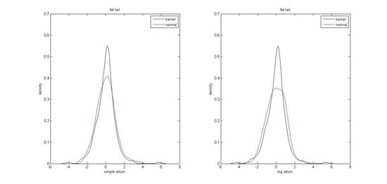
Empirically, we present two figures as an example for real-world data. The real data is the daily Tableau Software close price data from 15 March 2018 to 14 March 2019 collected via Yahoo! Finance at https://au.finance.yahoo.com/quote/DATA/history?p=DATA. Figure 2 shows its time series plots, with the upper panel for the simple returns and lower panel for the log returns. Figure 3 compares the empirical Tableau densities with normal densities and shows that the Tableau data reveals obviously a fat tail and high peak.
The initial studies that followed the seminal work of Mandelbrot (1963) used the stable Pareto distribution to simulate the fat tail of such data. Fama (1965), Fama and Roll (1968) also used stable Pareto distribution to study the fat tail characteristics of financial data. Such distributions have many properties exhibited by normal distribution such as closeness under summation. However, Upton and Shannon (1979) as well as Friedman and Vandersteel (1982) claimed that a stable Pareto distribution was inappropriate for simulating the fat tail shape of financial data because the return was more peaked and had fatter tails. Ghose and Kroner (1995) found that the GARCH model and the stability model had something in common, which meant that many of the discoveries of the stable distributions with fat tail in finance were caused by temporary volatility aggregation.
Subsequently, Sornette et al. (2000) introduced a multivariate fat tailed asset return distribution and depicted accurately the high-order cumulants of wealth changes in arbitrary portfolios. A computational technique of functional integrals and Feynman diagrams borrowed from particle physics was used. Most of the empirical applications of the stochastic volatility (SV) model assume that the conditional distribution of returns, given the latent volatility process, is normal. Liesenfeld and Jung (2000) used German stock data to compare stochastic volatility model based on conditional normal distribution and conditional fat tail distribution. These conditional fat tail distributions were mainly Student t distributions and generalized error distributions. Cont (2001) presented a set of stylized empirical facts (including fat tail) emerging from the statistical analysis of price variations in various types of financial markets and analyzed how these stylized empirical facts invalidated many of the common statistical approaches. Chib et al. (2002) discussed a class of generalized stochastic volatility models defined by the horizontal effects of fat tails, fluctuations, observational and evolutionary equations, and the covariate effects of the jumping part of the observational equation and provided two Markov Chain Monte Carlo (MCMC) fitting algorithms for the above models. In addition, simulation-based inference in generalized models of stochastic volatility was considered.
Zhou (2002) used the multivariate normal mixture model to characterize the fat tail characteristics of market risk factors, examined the relationship between risk and return, and established an asset pricing model with fat tail characteristics excluding options. This model provided a new perspective to study asset pricing. Wong et al. (2009) proposed Student t mixture autoregressive model which is also able to capture serial correlations, time-varying means and volatilities, and the shape of the conditional distributions can be time varied from short-tailed to long-tailed, or from unimodal to multimodal. Also, Chen and Yu (2013) proposed a novel nonlinear VaR method to model the risk of option portfolio under fat tailed market risk factors. Multivariate mixture of normal distributions was used to depict the heavy-tailed market risk factors.
Glasserman (2004) used multivariate t distribution to characterize the risk factors of fat tailed market, and indirectly obtained an expression of closed moment generating function. This expression reflects the change of portfolio value when the fat tailed problem was transformed into thin tailed problem. On this basis, the moment generating function was obtained by using the structure of multivariate t distribution. Albanese et al. (2004) used multivariate t distribution to characterize the fat tail of market risk factors. First, the matrix transformation of option portfolio value was derived from Delta-Gamma-Theta model. Thereafter, the density function of option portfolio value was discretized. Finally, the approximate VaR value was calculated by Fourier inverse transformation and linear interpolation. This new method does not assume that the characteristic function for the return model is known explicitly. Considering the difference between multivariate normal distribution and multivariate t distribution in the description of market risk factors, Albanese and Campolieti (2006) proposed the probability density function for calculating the change of option portfolio value and the Monte Carlo simulation method for estimating the multivariate VaR at a given confidence level and explored the relationship between a normal distribution and a fat tail distribution. Like Glasserman (2004), Johannes et al. (2009) deduced the closed expression of moment generating function in the case of multivariate t distribution and compared Fourier-Inversion method with Monte Carlo simulation method. The results showed that the Fourier-inversion method was much quicker than Monte Carlo simulation method and that Fourier-Inversion was a good way to calculate option VaR. Asai (2008) studied two models for describing fat tail and volatility dependence: autoregressive stochastic volatility model with Student t distribution (ARSV-T) and multifactor stochastic volatility (MFSV) model, and the results showed that ARSV-T model provided a better fit than MFSV model based on Akaike Information Criterion (AIC) and Bayesian Information Criterion (BIC).
Asai (2009) compared stochastic volatility models defined by normal distribution and other fat tailed distributions, such as Student t distribution and generalized error distribution. Delatola and Griffin (2013) proposed a Bayesian semiparametric stochastic volatility model, and this model allowed the distribution of returns to be fat tail and allowed the correlation between returns and fluctuations. Abanto-Valle et al. (2015) proposed a stochastic volatility model which assumed that the return followed the biased Student t distribution. This model could flexibly control the skewness and the fat tail distribution of the return condition. Meanwhile, an effective MCMC algorithm was given to estimate and predict the parameters. Lafosse and Rodríguez (2018) combined stochastic volatility model with GH Skew Student t distribution to characterize the skewness and fat tail of financial data and showed the evidence of asymmetries and heavy tails of daily stocks returns data. Gunay and Khaki (2018) noted that capturing conditional distributions, fat tails and price spikes was the key to measuring risk and accurately simulating and predicting the volatility of energy futures. These researchers tried to model the volatility of energy futures under different distributions.
2.2. The Dependence of Financial Data
Financial data are usually interdependent. They also exhibit a tendency of volatility clustering, that is, temporal dependence, in which large financial returns are followed by large financial returns. The interdependence of financial data has been extensively researched in various fields of finance, for example, following the US stock market crash of 1987, the contagion spread to the UK and other developed countries (King and Wadhwani 1990). To model the non-linear dependence in data, following Engle (1982), many ARCH-type models have been proposed. However, assumption of iid in such models makes their use inappropriate to model non-linear dependence in a univariate series or simultaneous dependence in two or more timeseries. Copula comes to rescue here. Some important publications are listed in the following table.
Copula proposed by Sklar (1959) can identify the dependency structure, capture the potential nonlinear correlation, and fit the dependency of financial data well, which makes it a good choice to measure correlation (Embrechts 1999). Copula refers to “functions that join or couple multivariate distribution functions to their one-dimensional marginal distribution functions” (Nelsen 1999, p. 1). The copula decomposes an n-dimensional distribution function in to the marginal distribution functions and the dependence part. It is the latter that the copula describes. In Table 1 below some key research work on copula has been included.
“Modern risk management calls for an understanding of stochastic dependence going beyond simple linear correlation” (Embrechts et al. 2001). These researchers emphasized the necessity to use Copula to simulate multivariate correlations in financial data given its stochastic dependence and pitfalls. Mashal and Zeevi (2002) showed that Student t Copula had an advantage over other multivariate Copulas in fitting financial data. Kole et al. (2007) used goodness-of-fit test for t, Gaussian and Gumbel Copula in risk management of linear assets and found that t Copula had more advantages than Gaussian and Gumbel Copula. Sak et al. (2010) used a flexible and accurate model, such as t Copula dependency structure and generalized hyperbolic distribution, to simulate logarithmic returns. They also calculated the tail probability of the current asset portfolio.
Studies have shown evidence of two types of asymmetries in the joint distribution of stock returns: skewness in the distribution of individual stock returns and an asymmetry in the dependence between stocks. Patton (2004) showed that the rotational Gumbel Copula function was superior than the normal and the Student t Copula, in describing the asymmetric dependency structure of two stock indexes. Trivedi and Zimmer (2006) considered the use of the copula approach for a model with three jointly determined outcomes. The model could handle the discrete case in which outcomes include a mixture of dichotomous choices and discrete count data. They applied this technique to study self-selection and interdependence between health insurance and health care demand among married couples. Hu (2006) proposed a hybrid Copula+ model to capture different types of dependent structures, in which the marginal distribution of each market asset was estimated by nonparametric method and the mixed Copula was estimated by quasi-maximum likelihood method. Patton (2006) extended the Copula theory to allow conditional variables, analyzed two important exchange rates using different forms of Copula-GARCH model, and used them to construct a flexible model of conditional dependency structure of these exchange rates. Liu and Luger (2009) adapted and examined an iterative (fixed-point) algorithm for the maximum-likelihood estimation of copula-based models that circumvents the need to compute second-order derivatives of the full-likelihood function. The algorithm exploits the natural decomposition of a potentially complicated likelihood function: the first part is a working likelihood that only involves the parameters of the marginals and the residual part is used to update estimates from the first part.
Van den Goorbergh et al. (2005) studied the price problem of Binary Options with correlations between assets and used the parameter Copula family with multiple alternative Gaussian dependency structures to fit the correlation. The relationship was assumed to be a function of asset volatility and it changed with time. Since then, time-varying Copula model has been extensively studied. Bartram et al. (2007) used the time-varying Copula model to study the effect of the introduction of the euro on the dependence between 17 European stock markets from 1994 to 2003. The time-varying Copula model used the GJR-GARCH-T model to realize the marginal distribution and Gauss Copula to realize the joint distribution. These could capture the time-varying nonlinear correlations. The correct modeling of non-Gaussian dependences is a key issue in the analysis of multivariate time series, Giacomini et al. (2009) used copula functions with adaptively estimated time-varying parameters for modeling the distribution of returns and applied it to the portfolio VaR. Hafner and Reznikova (2010) proposed a new semiparametric dynamic Copula model in which the marginal of Copula was assigned as a parameter GARCH-type process while the dependent parameters of Copula could change with time in a nonparametric manner. Negative extreme changes were common in international stock markets, Garcia and Tsafack (2011) pointed out the limitations of some common methods and proposed a regime-switching Copula model, which included a normal system with symmetric dependencies and an asymmetric dependency. The system was applied to allow changes in the market between the international stock and bond markets. Hafner and Manner (2012) proposed a dynamic Copula model in which dependent parameters followed an autoregressive process. Since this kind of model includes Gaussian Copula with stochastic correlation process, it can be regarded as a generalization of multivariate stochastic volatility model. Mendes and Marques (2012) found that the dependency structure between assets was not only linear but also used robust estimation of dual Copula model to fit logarithmic returns. Chen and Tu (2013) used four different types of time-varying Copula to fit the index futures and spot returns by relaxing the traditional normal joint distribution hypothesis and improved the hedging portfolio VaR. Creal and Tsay (2015) constructed a series of Copula families with time-varying dependent parameters by writing Copula as a factor model with random loads.
The Vine Copula (Joe 1997) has great advantages in describing the relationship between multiple financial assets and is widely used in financial risk management. Maugis and Guegan (2010) compared the Vine Copula method with several traditional GARCH models and concluded that the Vine Copula method could give better portfolio VaR prediction. As distinct from the existing Vine Copula structure strategy, DiβMann et al. (2013) proposed automatic Copula selection and estimation technology based on graph theory. It enabled flexible modeling of complex dependencies, that is, even those with larger dimensions. So and Yeung (2014) discussed the construction+ of Vine Copula structure and studied the relationship between financial markets and Vine Copula theory. Geidosch and Fischer (2016) confirmed the advantages of Vine Copulas over traditional Copula in simulating the dependent structure of credit portfolios. Aiming to measure risk and finding the optimal weights of portfolios containing three financial instruments, Pastpipatkul et al. (2018) used C-D vine Copulas method to establish the dependence relationship of each pair of financial instruments and used Monte Carlo simulation technology to generate simulation data to calculate risk value (VaR) and expected shortfall.
3. Portfolio Selection: A Review of Common Models
A commonly used model for portfolio selection is the mean-variance model, in which, the optimal portfolio weight depends on the mean and covariance matrix of asset returns. Usually, the available portfolio weights are obtained by using sample mean and sample covariance matrix to replace the true mean and covariance matrices of asset returns respectively. However, the estimation of sample means, and covariance usually involves errors and the estimation errors in sample mean are much larger than those in sample covariance. This makes the mean-variance model more sensitive to estimation errors. Therefore, the global minimum variance models whose optimal portfolio weight only depends on the covariance matrix is used. Furthermore, for the measurement of portfolio risk, the factor model is commonly used to estimate covariance matrix.
Accordingly, the literature on portfolio selection has developed in three strands: the traditional mean-variance model and the newer, global minimum variance model and the factor model.
3.1. Mean-Variance Model
In the traditional mean-variance model proposed by Markowitz (1952), the return of financial assets is represented by a random variable with Gaussian distribution. The assumption of normal (Gaussian) distribution means that the return of assets depends only on the mean and variance. Markowitz (1959) extended the mean-variance model in a pioneering book on portfolio selection. Merton (1972) studied the application of the mean-variance model allowing short-sale in portfolio selection. Over the years, many studies have used the above models. Some groundbreaking articles are summarized in Table 2 below.
Markowitz’s traditional mean-variance model is a static model in which investors can only make investment decisions at the beginning of the investment period and then wait until the end of the investment period. Based on this, the mean-variance model was later extended to the multi-period case. Samuelson (1969) proposed a discrete time multi-period consumption-investment model to maximize the end-of-term expected utility for investors. Grauer and Hakansson (1993) compared the effects of mean-variance asymptotic and quadratic asymptotic in a discrete time dynamic investment model. Yi et al. (2008) used the mean-variance model to consider the discrete time portfolio optimization of asset liability management under uncertain investment level and deduced the analytical optimal strategy by using embedding technology. Wu and Li (2011) studied the discrete time mean-variance portfolio model with regime switching under the assumption of stochastic cash flow.
Merton (1969, 1971) studied the maximized expected return of continuous time model under a given planning period, which is a pioneering work of continuous time research. Karatzas et al. (1987) considered a generalized consumption-investment model with a single member, which aimed to maximize the linear combination of the total expected discount utility and the end-of-term wealth utility from the consumption over a continuous investment period. Li and Ng (2000) firstly used embedding technology to solve the problem of inseparability and constructed a framework with mean-variance model in a discrete case. Xie et al. (2008) used the stochastic optimal linear-quadratic control technique to obtain the optimal dynamic strategy for continuous time mean-variance portfolio selection in incomplete markets. Using dynamic programming and embedding techniques, the closed form optimal strategy and efficient frontier were derived. Xu and Wu (2014) studied the continuous time mean-variance portfolio selection problem with inflation in incomplete markets and obtained the efficient bounds of dynamic optimal strategy and mean-variance model. Wu and Chen (2015) studied the time-consistent multi-period mean-variance portfolio selection problem under the assumption that risk aversion was dynamically dependent on market conditions.
Pogue (1970) first gave a description of the mean-variance portfolio problem in the presence of transaction costs. Davis and Norman (1990) further explored the portfolio selection problem under proportional transaction costs. Dumas and Luciano (1991), Morton and Pliska (1995) studied portfolio selection with proportional transaction costs and fixed transaction costs, respectively. Yoshimoto (1996) first assumed that the transaction cost was a V-shaped function, and then obtained the optimal portfolio strategy. Oksendal and Sulem (2002) studied the optimal consumption and portfolio under fixed and proportional transaction costs, with the objective of maximizing cumulative consumption expected utility within the scope of planning. Xue et al. (2006) constructed a mean-variance portfolio selection model with concave transaction costs to capture real market conditions. The authors provide a branch and bound algorithm as a solution. Dai and Zhong (2008) proposed a numerical penalty method to solve the continuous time portfolio selection problem with proportional transaction costs. Peng et al. (2011) studied portfolio optimization with quadratic transaction costs in the framework of the mean-variance model. Wang and Liu (2013) studied the multi-period mean-variance portfolio selection problem with fixed and proportional transaction costs and defined the indirect utility function to solve the problem by using dynamic programming and Lagrange multiplier. Liagkouras and Metaxiotis (2018) proposed a new multi-period fuzzy portfolio optimization algorithm for multistage mean-variance fuzzy portfolio optimization with transaction costs.
To make the model more practical, different constraints were introduced in the mean-variance model. Fernández and Gómez (2007) generalized the standard mean-variance model including cardinality and boundary constraints, and the constraints guaranteed investment in a given set of different assets and limited the amount of capital invested in each asset. Soleimani et al. (2009) proposed a portfolio selection model based on mean-variance model framework, which included cardinality constraints, minimum trading lot sizes and market (sector) capitalization. Castellano and Cerqueti (2014) studied the mean-variance optimal portfolio selection problem for risky assets with low-frequency trading and low liquidity. To simulate the dynamics of illiquid assets, pure-jump processes were introduced, which enabled the development of portfolio selection models in mixed discrete/continuous time settings.
Simaan (2014) provided a framework that allowed performance comparisons of within and out of sample between mean-variance portfolios and portfolios that maximize expected utility. To develop the best market timing strategy, Gao et al. (2015) considered the mean-variance dynamic portfolio selection problem with management cost time constraints. Lioui and Poncet (2016) proposed a new portfolio decomposition formula to reveal the economics of investor portfolio selection according to the mean-variance criterion and noted that the number of components of the dynamic portfolio strategy could be reduced to two: the first was to hedge the risk of discounted bonds maturing within the investor’s time limit without preference, while the second was to hedge against time variation in pseudo relative risk tolerance.
3.2. Global Minimum Variance Model
The global minimum variance model (GMV) is a specific optimal portfolio with minimum variance on the effective boundary. Haugen and Baker (1991) used the GMV model to verify whether the capitalization weighted (cap weights) portfolio was an efficient investment as claimed by sponsors of such plans. These researchers found that even assuming informationally efficient capital market and that all investors rationally optimized the relationship between risk and expected return, the portfolio of cap weights was not efficient except under extreme restrictive conditions. Chopra and Ziemba (1993) promoted the use of GMV in finance and pointed out that the error in expected returns was 10 times than the error in variance and covariance. Chan et al. (1999) focused on the GMV portfolio and emphasized that the GMV portfolio performed better than the Markowitz mean-variance model. Jagannathan and Ma (2003) pointed out that the weight of the GMV portfolio should be more stable than that of the standard mean-variance model because the estimation error of the covariance was smaller than that of the mean. Kempf and Memmel (2006) noted that the GMV portfolio could provide better out-of-sample results than the tangent portfolio theory and studied the distribution of portfolio weights under the GMV model. DeMiguel and Nogales (2009) claimed that GMV model relied only on covariance matrices and were insensitive to estimation errors. These studies have led to the popularity of GMV in portfolios selection.
Traditional GMV only solves the portfolio weights from the perspective of optimization, but many scholars are interested in the distribution and nature of the portfolio weights of GMV. Under the assumption of normal distribution, Okhrin and Schmid (2006) derived the multivariate density function of GMV portfolio. Clarke et al. (2006) noted that the stock weights on the left of the effective boundary under the minimum variance model were independent of the expected safe return. At this point, the portfolio could be obtained only by using the covariance matrix of stocks without involving the equilibrium expectation or the active forecast return. Bodnar and Schmid (2008) discussed portfolio weights in GMV model under the assumption that returns followed a matrix elliptical contoured distribution. Assuming that securities returns were neither normal nor independent, they found that the stochastic nature of the portfolio in GMV model did not depend on the mean vector and the assumption of the distribution of securities returns. Bodnar and Schmid (2009) derived the variance and expected return of sample GMV portfolio distribution. Frahm (2010) derived a small sample hypothesis test for global and local minimum variance portfolios and calculated the exact distribution of portfolio weight estimation. At the same time, the first two moments of the estimation of portfolio expected return were given. On the assumption that the conditional distribution of logarithmic returns was normal, Bodnar et al. (2017) considered the weight estimation problem of the optimal portfolio from the perspective of Bayes and obtained the posterior distribution of the weight of GMV portfolio by using the standard prior of mean vector and covariance matrix.
Following the research on distribution and nature of the portfolio weights of GMV, parameter uncertainties, Glombek (2014) analyzed the mean, variance, weight and Sharpe ratio estimators of excess returns of GMV portfolio under consistent and asymptotic distributions, discussed the problem of high-dimensional assumptions and demonstrated the applicability of this method. Maillet et al. (2015) proposed a robust approach to mitigate the effects of parameter uncertainties for a decision maker using GMV strategy to optimize portfolio selection. Based on Taylor’s robust M-estimator and Ledoit-Wolf shrinkage estimator, Yang et al. (2015) proposed a hybrid covariance matrix estimator under the GMV model for portfolios, with outliers of financial data, fat tailed distribution of sample data and obtained a consistent estimate of portfolio risk by minimizing the optimum linear shrinkage strength using random matrix theory. Bodnar et al. (2017) analyzed the GMV portfolio model under the Bayesian framework, adding the prior beliefs of investors to the investment decision. Carroll et al. (2017) evaluated the performance of GMV portfolio strategy and equal weight portfolio strategy under time-varying conditions between assets. They found that conditional correlation is more important than conditional variance in portfolio performance. The also found that frequent asset rebalancing does not help improve portfolio performance. Bodnar et al. (2018) estimated the GMV portfolio in high-dimensional case by using the results of random matrix theory, gave a shrinkage estimator in the sense of non-distribution assumption and minimizing the variance of samples, and obtained the asymptotic properties of the estimator under the assumption of the existence of fourth-order moments.
The mean-variance models are highly data intensive. Consequently, search was on for models that can capture enough of reality but are simpler. This led to the development of factor models.
4. Factor Model
The literature on factor models has evolved in two stages: single factor models and multi-factor models.
A factor model that is linear in form posits that the return of an asset can be expressed by the following equation:
where r is the return of an asset, a, b1, …, bk are the parameters, e is the error term. We call it a single factor model when k = 1, and we call it a multi-factor model when k ≥ 2.
r = a + b1f1+ ⋯ + bkfk + e,
4.1. Single Factor Models
The factor models have drawn attention of researchers, after Sharpe (1963) used, the factor model to estimate the covariance matrix. Geweke (1977) used dynamic factors to analyze the economic time series data and found that the results supported the methodology.
Geweke and Singleton (1981) proposed the theory of identification, estimation and inference in the dynamic confirmatory factor model of economic time series data and pointed out that the dynamic confirmatory factor model could accommodate the important characteristics of prior constraints in the parameter matrix. Watson and Engle (1983) studied the problem of specification and estimation of the dynamic unobserved component model and provided the method of estimating unknown parameters based on score method and EM algorithm by maximizing the likelihood function. Diebold and Nerlove (1989) identified and estimated the univariate ARCH model, and then used the results of the univariate ARCH model to propose the multivariate latent variable ARCH model. Engle et al. (1990) suggested the use of Factor-ARCH model as a concise structure of conditional covariance matrix of asset excess returns, which made it possible to study the dynamic relationship between asset risk premium and volatility in multivariate systems. Through a variety of diagnostic tests and compared with the previous empirical results, it was shown that the Factor-ARCH model was better as compared to other models given that it had the advantage of stability over time. Lanne and Saikkonen (2007) proposed a multivariate generalized orthogonal factor GARCH model and gave a program to test the correctness of the number of factors. Also, a mixture of Gaussian distributions was considered, and it was found that some parameters of the conditional covariance matrix that were not identifiable under normality could be identified when the mixture specification was used. Cardinali (2012) used orthogonal factors to model the structure of conditional covariance matrices. The advantage of this approach was that the estimated factors could be simulated using a univariate GARCH process, and the model could be extended to multivariate cases.
4.2. Multi-Factor Models
Litterman and Scheinkman (1991) empirically determined the common factors of treasury bond returns based on past securities. The analysis showed that most of the fluctuations of fixed income securities return could be explained by three factors, and the three-factor model was particularly useful for hedging. Chen and Scott (1993) considered that it was necessary to establish a formal theoretical structure model for bonds and other different types of interest rate options. Based on this, a multi-factor equilibrium model was proposed to estimate the parameters driving the interest rate change process and to determine the number of factors necessary to characterize the interest rate structure model. Duffie and Kan (1996) proposed a consistent and arbitrage-free multifactor model of the term structure of interest rates. The model assumed that the returns on a fixed maturity date followed a parametric multivariate Markov diffusive process with stochastic volatility parameters and provided the necessary and sufficient condition for numerical algorithm and the stochastic affine representation of the model. Fama and French (1993) proposed that the return on excess assets could be explained by three factors: sensitivity to market excess returns, market capitalization and book price ratio. Campbell (1996) noted that adding human capital to common factors could improve the performance of multi-factor asset pricing model in predictability of returns. Chan et al. (1999) found that the market, size and stock market value can capture the common structure of the return covariance matrix and found that the use of three factor model for the minimum variance portfolio model was adequate. Stock and Watson (2002) studied predictions with multiple predictors, observations, and a single time series, and noted that a small number of principal component estimators could be used for prediction when data followed an approximate factor model. Bai (2003) used principal component estimator to establish the inference theory of large-dimensional factor model and derived the finite distribution of convergence rate and factor, factor load and common component. Han (2006) studied the effects of time-varying expected return and volatility on asset allocation in a high-dimensional context, and proposed a dynamic factor multivariate stochastic volatility model, which allowed the first two moments of many assets returns to change with time. Adrian and Franzoni (2009) used conditional CAPM models to allow unobserved changes in risk load factors over time. Based on the assumption that investors could rationally learn the long-term level of the load factor from the observed returns, Kalman filter was used to simulate conditional beta. Fan et al. (2013) used the multifactor model to estimate the covariance matrix in the high-dimensional case. Jungbacker et al. (2014) studied the dynamic factor model and showed how to use cubic spline function to smoothly limit the factor load. Hou et al. (2015) put forward a new four factor model by combining market and scale with investment and profitability. Jungbacker and Koopman (2015) presented a new method of dynamic factor model based on likelihood analysis. These researchers used linear dynamic stochastic processes to simulate latent factors and autoregressive processes with correlations to determine the singular perturbation sequence. The method was found to be effective in estimating the factors and maximum likelihood parameters. Fama and French (2015) added profitability and investment to the three-factor model and constructed a five-factor model to reveal several abnormal phenomena of average returns. Fama and French (2016) used five-factor model to explain the abnormal phenomenon of average returns. Chiah et al. (2016) confirmed that the five-factor model was superior to the multifactor model in explaining the changes of asset returns in global asset market. Stambaugh and Yuan (2017) proposed a four-factor model that combined the two mispricing factors with market and size factors. They found that the ability of the model to account for many anomalies is much better than the earlier models.
Fama and French (2017) used international data to test the five-factor model. The global three factor and five factor models did not perform well in the test of regional portfolio. Therefore, local variables were used to establish the model that is, the factors and returns to be explained came from the same region. Kubota and Takehara (2018) used five factor model (Fama and French 2015) to test whether the model could well explain the pricing structure of Japanese long-term data stocks. They found that the original version of the five-factor model was not the best benchmark pricing model for Japanese data from 1978 to 2014. Roy and Shijin (2018) proposed a balanced six factor asset pricing model, which explained the change of asset returns by adding human capital to the five-factor model and tested the six-factor asset pricing model with four different portfolios. Tu and Chen (2018) developed a new factor-augmented model for calculating the value at risk (VaR) of bond portfolios based on the Nelson-Siegel structural framework and tested whether the information contained in macroeconomic variables and financial stress shocks could enhance the accuracy of VaR prediction.
5. Portfolio Risk Measure
Several methods are available for the measurement of portfolio risk and we divide them into (a) moment-based risk measurement and (b) moment-based and quantile-based risk measurement. The moment-based methods include time-varying covariance matrix and the shrinkage estimation use the covariance matrix in the risk measurement. The semi-variance method calculates the risk below the target value, and the target can be regarded as a quantile. VaR is based on quantile measures of risk, while CVaR is a measure of risk based on the idea of VaR quantile and mean value. Therefore, semi-variance, VaR and CVaR are risk measures based on moments and quantiles.
5.1. Moment-Based Risk Measurement
5.1.1. Time-Varying Covariance Matrix
Some groundbreaking publications are summarized in Table 3 below.
Engle (1982) introduced the autoregressive conditional heteroscedasticity (ARCH) family model and used it to estimate the means and variances of inflation in the U.K. The ARCH effect is found to be significant and the estimated variances increased substantially during the chaotic 1970s. Bollerslev (1986) extended the ARCH family model to the Generalized autoregressive conditional heteroskedasticity (GARCH). To capture the dynamic changes of financial markets, time-varying dynamic covariance matrix has been widely used in portfolio investment. Since the GARCH model can successfully describe one-dimensional time-varying variance, many researchers have tried to extend the time-varying variance to the multivariate case by using the multivariate GARCH model.
Bollerslev et al. (1988) used multivariate GARCH (MGARCH) model to estimate the earnings of bills, bonds and stocks. The expected return of bills, bonds and stocks was proportional to the return of each diversified or market portfolio. The results showed that conditional covariance varied greatly over time and this time-varying factor was an important determinant of time-varying risk premium. Kroner and Claessens (1991) used similar technologies to get a series of optimal dynamic hedge funds. Lien and Luo (1994) assessed the multi-period hedging ratio of currency futures in the framework of MGARCH.
Engle et al. (1984) provided a necessary condition for the conditional covariance matrix in the two-dimensional ARCH model to be a positive definite. However, it was not feasible to extend the necessary condition of positive definite conditional covariance to a more generalized model. Bollerslev (1990) suggested that the constant conditional correlations (CCC) MGARCH model could overcome the difficulty of positive definite. Because of the simplicity of calculation, constant conditional correlations MGARCH model has been widely used in practice, but some researchers find that some assumptions of constant correlations MGARCH model are not supported by financial data in practice. Engle and Kroner (1995) gave the formulas and the theoretical results of estimations for multivariate GARCH models in simultaneous equations, proposed a new parameterization method (BEKK) for multivariate ARCH processes, and discussed the equivalent relations of various ARCH parameterizations. At the same time, the sufficiency constraints for the conditional covariance matrix to guarantee positive definiteness were proposed, and the ‘sufficient and necessary conditions’ for the stability of covariance were given.
Bera et al. (1997) pointed out that the BEKK model proposed by Engle and Kroner (1995) did not perform well in estimating the optimal hedging ratio. Also, Lien et al. (2002) pointed out that BEKK was difficult to converge in estimating the conditional variance structure of spot and futures prices. Tsui and Yu (1999) used the dual GARCH model to study stock returns in two emerging markets, Shanghai and Shenzhen of China, and the information matrix test statistic did not support the hypothesis of the constant conditional correlation of stock returns. Tse (2000) introduced the Lagrange Multiplier test to the multivariate GARCH model with constant correlation assumption and this test verified the limitations of the multivariate GARCH model with constant correlation. The data of stock market returns in China was used to draw a conclusion that the correlation was time-varying.
The fact that the correlation is time-varying has been accepted by many scholars. Tse and Tsui (2002) proposed a MGARCH model with time-varying correlation. The conditional covariance matrix could be decomposed into conditional variance matrix and conditional correlation coefficient matrix. Each conditional variance term was assumed to follow a unitary GARCH model, and the conditional correlation coefficient matrix followed a similar autoregressive moving average. At the same time, Engle (2002) proposed a new family of multivariate GARCH models, a dynamic conditional correlation (DCC) model to estimate time-varying correlations.
MGARCH model settings are usually determined by practical considerations such as easy estimation, which often leads to serious losses in general. The deficiencies and developments on the DCC and BEKK models have been extensively reviewed by McAleer (2019a, 2019b). Alexander (2001) proposed an orthogonal GARCH model in which the time-varying covariance matrix was derived from a small number of uncorrelated factors. Van der Weide (2002) proposed a new MGARCH model: the covariance matrix with many parameters could be parameterized with considerable degrees of freedom and the estimation of parameters was still feasible. This model could be regarded as a natural generalization of O-GARCH model and nested in a more general BEKK model. To avoid the difficulty of convergence, the unconditional information was used to make the number of parameters estimated by conditional information more than half. Vrontos et al. (2003) proposed a new parameter method for MGARCH with time-varying covariance: the covariance matrix guaranteed positive definiteness and the number of parameters of the method was relatively small, which could be easily applied to high-dimensional time series data model. The parameter estimation of multivariate model was realized by classical Bayesian technique, and the maximum likelihood estimation was realized by Fisher scoring method. Ledoit et al. (2003) proposed a new method for estimating the time-varying covariance matrix in the framework of the MGARCH (1,1) model for the diagonal VECH. This method was numerically feasible in dealing with large-scale problems and could generate semi-definite conditional covariance matrix without imposing impractical prior restrictions.
Cappiello et al. (2006) studied the existence of asymmetric conditional second-order moments in international equity and bond yields and analyzed them by the asymmetric version of Engle (2002) dynamic conditional correlation (DCC) model. A large amount of evidence showed that the series of national stock index returns indicated strong asymmetric conditional volatility, while there was little evidence that bond index returns showed such behavior. McAleer et al. (2008) established the generalized autoregressive conditional correlation (GARCC) model on the assumption that the normalized residual followed the random coefficient vector autoregressive process. The GARCC model enabled conditional correlation to change over time. GARCC was also more general than Engle (2002) Dynamic Conditional Correlation (DCC) and Tse and Tsui (2002) time-varying correlation model and did not impose excessive restrictions on the parameters of DCC models. At the same time, the structural properties of GARCC model, especially the analytical form of regularity conditions, were deduced, and the asymptotic theory was established. Hafner and Franses (2009) extended Engle (2002)’s DCC model to allow asset-specific correlation sensitivity. This model was useful for investors holding large asset returns. At the same time, they proposed two estimation methods, one based on complete likelihood maximization and the other based on individual correlation estimation. Applying the generalized DCC (GDCC) model to the daily data of stock returns of 39 UK firms on FTSE, they found convincing evidence that the GDCC model was improved on the DCC model and on the constant conditional correlations MGARCH model of Bollerslev (1990). Haas et al. (2009) proposed an asymmetric multivariate extension of a new normal mixed GARCH model, discussed the parameterization and estimation problems, derived the covariance stationarity condition and the existence of the fourth moment, and gave the expression of the dynamic correlation structure of the process.
Diamantopoulos and Vrontos (2010) used multiple Student t error distributions to simulate the fat tail nature of conditional distribution of financial returns data, extended the Vrontos et al. (2003) model, and then proposed a Student t full factor multivariate GARCH model. Combined with the reduction parameterization of covariance matrix in the full factor multivariate GARCH model, the model could be applied to high dimensional problems. Ausin and Lopes (2010) argued that the conditional ellipsoid joint distribution of MGARCH model required strong symmetry, and financial data did not satisfy this assumption in many cases. Therefore, they proposed a time-varying correlation Copula GARCH model to deal with portfolio selection problems. Wei et al. (2010) used a greater number of linear and nonlinear GARCH class models (see McCulloch (1985); Polasek et al. (2007) to capture the volatility features of two crude oil markets and found that the nonlinear GARCH-class models exhibited greater forecasting accuracy than the linear ones. Christoffersen et al. (2012) combined the DCC model with partial t Copula to study the conditional correlation of emerging stock market indices in 33 developed countries. Santos and Moura (2014) proposed a new method for conditional covariance matrix estimation based on flexible dynamic multivariate GARCH model.
Klein and Walther (2016) incorporated an Expectation-Maximization algorithm for parameter estimation of the mixture memory GARCH (MMGARCH) and found MMGARCH was also able to cover asymmetric and long memory effects. Also, for variance forecasting and Value-at-Risk prediction, they found MMGARCH performed better due to its dynamic approach in varying the volatility level and memory of the process. Conrad and Mammen (2016) established the asymptotic theory of quasi-maximum likelihood estimator for the parametric GARCH-in-Mean model. The asymptotic behavior was based on the study of fluctuations of the parametric process of the model. Although time-varying GARCH-M models are commonly used in econometrics and finance, the recursive nature of conditional variance makes likelihood analysis computationally infeasible. Therefore, Anyfantaki and Demos (2016) suggested using Markov Chain Monte Carlo algorithm, which allowed classical estimators to be computed by simulating EM algorithm or only using simulated Bayes in O(T) operations (T is sample size), and derived the theoretical dynamic properties of time-varying parameter EGARCH (1,1)-M. Dias (2017) proposed an estimation strategy for stochastic time-varying risk premium parameters in time-varying GARCH-in-mean model, and Monte Carlo study showed that the algorithm had good finite sample properties.
Although time-varying covariance matrix performs well in capturing the dynamic change of finance markets, sample covariance matrix is used to replace the truly unknown covariance matrix in practice and there is estimation error in sample covariance matrix. Therefore, shrinkage estimation is introduced to reduce estimation error in sample covariance matrix.
5.1.2. Shrinkage Estimation
Jobson and Korkie (1980) used James-Stein estimator in mean-variance portfolio to demonstrate that the estimator provides more reasonable results than the traditional estimators. Jorion (1985) revealed the disadvantages of replacing expected returns with corresponding sample estimate without considering the inherent uncertainty in these parameter values. On this basis, Stein’s method of estimating initial returns was studied. By shrinking the sample average to a common mean, it was found that the out-of-sample performance of the optimal portfolio increased significantly. Frost and Savarino (1986) studied the portfolio selection problem by maximizing expected returns, based on the forecasting distribution of securities returns under the Bayesian framework, and found that the method could improve the performance of portfolio by reducing the priori information of estimation error. Jorion (1991) compared the active investment strategies of expected return under three alternative models: historical sample mean, shrinkage or Bayesian estimation and CAPM-based estimation and found that exchange risk is not factored in to stock prices despite its significance. Like Jorion (1991), Grauer and Hakansson (1995) compared the investment strategies and returns of the three estimated dynamic investment models. Mori (2004) studied the performance of mean-variance model on the optimal portfolio weights of proportional estimator and Stein estimator when the parameters were unknown. Kan and Zhou (2007) discussed the problem of investing in riskless assets and tangent portfolio funds and proposed a combination of sample tangent portfolio and sample global minimum variance portfolio. Okhrin and Schmid (2007) provided a comparison between the exact and asymptotic distributions of portfolio weight estimates and a sensitivity analysis of asset return moments. At the same time, considering the shrinkage estimation of several types of moments, the portfolio weights and its corresponding estimators were compared based on moment estimation.
The use of linear shrinkage to estimate covariance matrix has also attracted wide attention among researchers. Ledoit and Wolf (2003, 2004) used a linear combination of sample covariance matrices and a target matrix to estimate the covariance matrix, where the target matrix could be the identity matrix, or the covariance matrix estimated by the one factor model and applied this method to the portfolio selection problem. Bai and Shi (2011) summarized the methods commonly used in high-dimensional covariance matrix estimation, including shrinkage, observable and implicit factors, Bayesian method and random matrix theory. Yang et al. (2014) proposed a hybrid covariance matrix estimation method based on robust M estimation and Ledoit and Wolf (2004) shrinkage estimation. Ikeda and Kubokawa (2016) considered a class of general weighted estimators, including the linear combination of sample covariance matrices and the model-based estimators and the linear shrinkage estimators without special factors under the factor model.
On the other hand, the optimal portfolio is directly dependent on the inverse of the covariance matrix. Accordingly, the direct shrinkage of the inverse covariance matrix is also a good strategy. Stevens (1998) dealt with portfolio optimization problems by primitively constructing several direct characteristics of the inverse covariance matrix. Kourtis et al. (2012) used the linear combination of the inverse covariance matrix and the target matrix to estimate the inverse covariance matrix, where the target matrix could be the identity matrix, the inverse of the covariance matrix estimated by the one factor model and the linear combination of the former two and applied this method to the portfolio selection problem. Bodnar et al. (2016) gave an explicit stochastic representation of the weights of mean-variance portfolios by using the linear transformation distribution of the inverse covariance matrix.
Bickel and Levina (2008a) discussed the regularization of covariance matrices with n observation samples and p variables by hard threshold method. Under the conditions that: the true covariance matrix was sparse in a proper sense, the variables were Gaussian or sub-Gaussian distribution, (Log p)/n approached zero and the explicit rate could be obtained, then the threshold estimation was consistent. Bickel and Levina (2008b) studied the estimation of banded and tapered sample covariance matrix and the banded inverse covariance matrix. Rothman et al. (2009) proposed a new generalized threshold algorithm combining shrinkage and threshold and studied the generalized threshold of sample covariance matrix in high-dimensional case. The generalized threshold of the covariance matrix has good theoretical properties and almost no computational burden. At the same time, an explicit convergence rate can be obtained in the operator norm, showing the tradeoff between sparsity, dimensionality and sample size of the real model. It was found that the generalized threshold is consistent in a large class of models if the dimension p and sample size n satisfy log (p/n) approaching zero. Konno (2009) considered the estimation of large-dimensional covariance matrices for multivariate real normal and complex normal distributions when the dimensions of variables were larger than the number of samples. For real and complex cases, the Stein-Haff equations and eigen structures of singular Wishart matrices were respectively, provided. By using these techniques, unbiased risk estimates for some classes of global covariance matrices under real and complex invariant quadratic loss functions were obtained. Chen et al. (2010) considered the shrinkage method in a high-dimensional case and, proposed a covariance estimation method based on minimizing mean square error in Gaussian samples. Firstly, under the condition of sufficiency of statistics, Rao-Blackwell theory was used to propose a new method, RBLW estimator, which was superior to Ledoit-Wolf method under mean square error. Secondly, the iterative method of the clairvoyant shrinkage estimator was proposed to reduce estimation error. At the same time, the convergence of the iterative method was established, the closed-form expression of the limit was determined, and this method was an Oracle approximate contraction (OAS) estimator. Fisher and Sun (2011) used the convex combination of the sample covariance matrix and the well-conditioned target matrix to estimate the covariance matrix and introduced a new set optimal convex combination estimates of three commonly used target matrix. Cai and Liu (2011) considered the estimation of sparse covariance matrix using the threshold step of single element change. The estimator is completely data-driven and has good data and theoretical results. Moreover, the estimator adaptively achieves the optimal convergence rate on a large class of sparse covariance matrices under spectral norm. Ledoit and Wolf (2012) further studied the linear shrinkage of Ledoit and Wolf (2004) by nonlinear transformation of sample eigenvalues and extended the nonlinear shrinkage method to the precision matrix. Fan et al. (2013) proposed the principal orthogonal complement thresholding method (POET) to discuss the estimation of high-dimensional covariance with conditional sparse structure and fast divergent eigenvalues. By assuming the sparse error covariance matrix in the approximate factor model, some cross-sectional correlations were allowed even after the common but unobservable factors were excluded. The POET estimator included sample covariance matrix, factor covariance matrix, threshold estimator and adaptive threshold estimator. At the same time, the convergence rates of sparse residual covariance matrix and conditional sparse covariance matrix under different norms were studied. With the increase of dimension, the sample covariance matrix becomes ill-conditioned and even singular. A commonly used method to estimate covariance matrix is Stein-type type compression estimation when the dimension is high. Touloumis (2015) proposed a new family of nonparametric Stein-type shrinkage covariance estimators, which were convex linear combinations of sample covariance matrices and predefined reversible target matrices. Under the Frobenius norm, the optimal shrinkage strength for defining the optimal convex linear combination depended on the unobserved covariance matrix and must be estimated from the data. At the same time, a simple and effective estimation process was proposed, which could obtain the nonparametric uniform estimator of the optimal contraction intensity for three commonly used target matrices. Zhang and Zhang (2018) combined the advantages of shrinkage estimation, vine copula structure and Black-Litterman model that could satisfy three investment objectives: estimation sensitivity, asymmetric risks appreciation, and portfolio stability.
5.2. Moment-Based and Quantile-Based Risk Measurement
5.2.1. VaR and CVaR
Some important articles are summarized in Table 4 below.
With the in-depth study of portfolio optimization theory and financial data, VaR attracted increasing attention in risk measurement. Baumol (1952) put forward the idea of VaR and used it to study the choice of securities. After Morgan (1996)’s risk measurement system, VaR has gained more attention (see Beder 1995; Jorion 1996). The basic principle recommended by the Basel Committee on Banking Supervision in 2001 states that VaR is a key indicator of risk (Szegö 2002). Goldfarb and Iyengar (2003) considered the robust VaR portfolio selection problem under the assumption of normal distribution and the objective of these robust formulations was to systematically combat the sensitivity of the optimal portfolio to statistical and modeling errors in the estimates of the relevant market parameters. Ghaoui et al. (2003) studied the portfolio selection problem with the worst case VaR when some of the distributed information was known. VaR is also used in insurance contracts. Wang et al. (2005) designed an optimal insurance contract by maximizing the expected final wealth of the insured under VaR constraints. Based on Wang et al. (2005), Huang (2006) established an insurance contract under the risk constraint of VaR assuming that the insured was risk-averse. Giot (2005) used GARCH model and Riskmetrics model with residuals following normal distribution and Student t distribution to study VaR of three stocks traded on NYSE in 15 and 30 min. Chin (2008) compared the power of VaR under quantile and nonlinear time-varying volatility, proposed a simple Pareto distribution to explain the fat tail property in the empirical distribution of return, and implemented the measure of non-parametric quantile estimation of VaR using interpolation method. Batten et al. (2014) used the modified version of the multifractal model of asset returns (MMAR) with a series of asset returns data characterized by second. Considering the fat tail of financial data, long-term dependence and inconsistency with the MMAR scale, the out-of-sample VaR prediction was derived, and the difference between this method and GARCH (1,1) position scale VaR model was compared. Zhao and Xiao (2016) proposed an optimal portfolio selection model with VaR constraints and the asset price process was modeled by a non-generalized statistical mechanics rather than a classical Wiener process. This model could describe the characteristics of fat tails of returns. Also, a Hamilton Jacobi Bell equation was obtained by using the dynamic programming principle and the closed form solution of logarithmic utility was obtained by Lagrange multiplier method. Jang and Park (2016) incorporated VaR constraints into the wealth and fuzziness of fund management and provided an optimal portfolio selection model for fund managers who divided assets into risk and risk-free. Chang et al. (2016) used the Granularity Adjustment (GA) method to calculate VaR in portfolio credit risk model and used Monte Carlo simulation to study the impact of concentrated risk on risk value. Naimy (2016) used CDS portfolio data from March 2013 to November 2015 in the United States, Europe and Asia to study the accuracy of VaR by measuring risk under the Delta normal and historical methods. Based on the VaR calculation method of portfolio composed of options and bonds, Wang et al. (2017) proposed a Monte Carlo simulation method to allow jump diffusion in underlying assets and provided a layout suitable for various models, including non-parametric and semi-parametric structures.
Several nonlinear VaR models for the calculation of option portfolio VaR have also been extensively studied. These models concentrate on relaxing the assumption that the change of option portfolio value is linear with the change of market risk factors while maintaining the computational feasibility. They improve the correlation between market risk factors and option portfolio value, including quadratic and linear terms, and are called Delta-Gamma-Theta-Normal VaR models. Morgan (1996) calculated the VaR value of option portfolio using the method of Johnson distribution transformation. Hardle et al. (2002) evaluated the accuracy and speed of computational methods for nonlinear VaR, including Johnson transformation, Cornish-Fisher, Monte Carlo and Fourier-Inversion methods. Data experiments showed that Johnson transformation and Cornish-Fisher method were faster but inexact, and Monte Carlo method was accurate but inefficient. Accordingly, the Fourier-Inversion method was found to be the best choice. Castellacci and Siclari (2003) used the Cornish-Fisher method to calculate the first-order moments of the distribution of portfolio value changes. Cui et al. (2013) studied Delta-Normal and Delta-Gamma-Theta-Normal VaR as well as parametric VaR asymptotic methods for nonlinear portfolios and discussed their computational effectiveness.
The widespread use of VaR has led many researchers to expand it to multidimensional case. However, there are many definitions of multidimensional quantile that make it difficult to generalize one-dimensional VaR to multivariate and still maintain many good properties of one-dimensional VaR (see Serfling 2002; Hallin et al. 2010; Fraiman and Pateiro-López 2012). In addition, McKay and Keefer (1996) believed that VaR may be ineffective in portfolio selection. Artzner et al. (1997) pointed out that VaR did not have subadditivity and convexity. Basak and Shapiro (2001) noted VaR-based optimal decisions had greater losses than expected expectation-based optimal decisions. Miller and Liu (2006) argued that under the current general assumption of joint normal distribution, there were many deviations in the VaR model of portfolio due to model set up errors.
Fortunately, Artzner et al. (1997) and Embrechts et al. (1999) explained that CVaR could be a reasonable alternative to VaR. Pflug (2000) proved that CVaR was a coherent risk measure and emphasized several properties of CVaR, such as convexity and monotonicity. Uryasev (2000) provided a comprehensive description of CVaR. Assuming the distribution was ellipsoid and the VaR was computable, Embrechts et al. (2001) showed the result of CVaR under the restricted condition was consistent with that of VaR. Rockafellar and Uryasev (2002) argued that CVaR was superior to VaR as a risk measure and gave the properties of CVaR under the distribution of financial losses involving prudent behavior. Gaivoronski and Pflug (2005) gave a method to calculate the minimum VaR portfolio under specific returns. By removing local outliers and smoothing VaR, the VaR’s efficient boundaries were calculated. At the same time, the differences of VaR, CVaR and standard deviation as risk measures were compared. Kibzun and Kuznetsov (2006) compared the standards of VaR and CVaR and identified the links between them. Topaloglou et al. (2008) used CVaR as a risk measure to solve the international portfolio selection problem under the stochastic programming model. Huang et al. (2010) considered the relatively robust CVaR model when the potential distribution of asset returns belonged to a particular set. Under the worst case of uncertain distribution, the possible optimal decision was given according to the realization of each distribution. Mainik and Schaanning (2012) compared two possible concepts of CVaR available in the current literature, studied their general dependency consistency, and presented their performance in several stochastic models. Nguyen and Samorodnitsky (2013) proposed a multivariate tail estimator involving CVaR sequential statistical tests. Bernardino et al. (2014) constructed two multivariate CVaRs at the level of multivariate distribution functions and provided new risk measures based on Copula structure and random ordering of marginal distributions. Wang and Huang (2016) endogenously formulated the best form of insurance contract to maximize the expected utility of insurance under VaR and CVaR constraints. Date and Bustreo (2016) studied how to approximate VaR and CVAR using new heuristic methods when the net return of portfolio investment may be a nonlinear function of non-Gaussian risk factors. Chen and Yang (2017) used CVaR as a risk measure to propose portfolio stochastic programming and stage wise portfolio stochastic programming based on the stock investment data. Zhang and Gao (2017) used the dynamic CVaR risk-constrained benchmarking process to deal with the dynamic portfolio problem. Using the dynamic programming technique, they derived the corresponding Hamilton Jacoby Bellman equation and obtained the optimal portfolio strategy by Lagrange multiplier method. Li et al. (2018) proposed a hybrid intelligent algorithm using genetic algorithm design and adaptive penalty function, Simulated Annealing Back Propagation neural network and fuzzy simulation technic to solve the fuzzy mean CVaR efficient portfolio model. At the same time, in order to further improve the computing speed, MPI technology was used to parallelize the hybrid intelligent algorithm.
For both the VaR and CVaR, a probability level of cumulative loss needs to be specified (Benninga and Wiener 1998). Furthermore, (i) the optimal portfolios with the VaR constraints are sensitive to the confidence level selected (Campbell et al. 2001), (ii) the CVaR model requires either an assumption about the asset returns distribution or a substantial amount of return observations below the target return (Boasson et al. 2011). Comparison with VaR and CVaR, semi-variance is a good substitution for measuring the one-sided risk.
5.2.2. Semi-Variance
Some groundbreaking articles are summarized in Table 5 below.
Roy (1952) proposed the concept of downside risk and defined it as a risk below the target value. Markowitz (1959) proposed a well-known mean-semi-variance model to estimate the weights of portfolio. Hogan and Warren (1972) pointed out the advantage of using the mean-semi-variance criterion in portfolio selection over the mean-variance model. Stone (1973) gave two interrelated three-parameter risk measures, in which the semi-variance was a special case. Hogan and Warren (1974) compared the difference between mean-variance model and mean-semi-variance model. Porter (1974) analyzed the relationship between stochastic dominance and mean-semi-variance model. Jahankhani (1976) empirically verified the relationship between return and risk in the mean-variance model and mean-semi-variance asset pricing model. Bawa and Lindenberg (1977) extended the semi-variance to the generalized lower partial moment framework, developed a Capital Asset Pricing Model (CAPM) using a mean-lower partial moment framework and derive explicitly formulae for the equilibrium values of risky assets that hold for arbitrary probability distributions. Fishburn (1977) applied the downside risk to the utility function model. Bawa (1978) extended the downside risk to higher order and showed its usability. Nantell and Price (1979) calculated variance and semi-variance by means of the distribution of prior portfolio returns and found that asset market portfolio prices with semi-variance were higher than variance at a certain risk level. Choobineh and Branting (1986) provided a simple form of semi-variance approximation by using mean, variance, critical value and cumulative probability below the critical value. Lee (1988) proposed a new asset pricing model in the framework of mean lower partial moment, which used semi-variance and semi-deviation to measure risk. Lewis (1990) used semi-variance as a measure of risk, applied it to the capital market and utility theory, and explained its advantages and disadvantages. Chen et al. (1991) proposed a set of linear regression models to approximate the semi-variance of the total returns of items with independent distribution. Chow et al. (1992) pointed out that in the absence of prior knowledge about the parametric structure of asset return distribution and the form of investor preference function, variance may no longer be an appropriate risk measure. They used various risk-return measures independent of distribution to test the efficiency and decentralization effect of international portfolio investment and found that semi-variance could effectively and conveniently identify risks. Tse et al. (1993) put forward an optimal strategy for personal investment using downside risk and proposed a model for accurate calculation of failure probability under the assumption of Brown’s motion process. Markowitz (1993) transformed the mean-semi-variance portfolio optimization problem into the mean-variance optimization problem and used the critical line algorithm to obtain the optimal solution. Josephy and Aczel (1993) proposed an unbiased, consistent and effective estimators for the semi-variance.
With the deepening of risk research, the downside risk has attracted more and more attention (Rom and Ferguson 1994). Kaplan and Alldredge (1997) used a specific risk-based index, which could maintain a certain level of risk in different periods of time, to make a series of trade-offs between risk and return and studied its properties and performance in the case of semi-variance. Hamza and Janssen (1998) took transaction cost into consideration and applied the mean-semi-variance model to the portfolio selection problem, introduced a series of binary variables and separable constraints, and finally solved the portfolio optimization problem using separable techniques. Grootveld and Hallerbach (1999) analyzed the similarities and differences of using variance and downside risk as risk measures from empirical data and theory. Costa and Nabholz (2002) considered different computational forms of mean and semi-variance with errors and formulated robust mean-semi-variance portfolio selection problems based on linear matrix inequality optimization problems. Estrada (2004) noted that semi-variance was supported by theoretical facts and practical considerations and was a feasible measure of risk, and that the mean-semi-variance behavior criterion was perfectly consistent with the expected utility and the average compound return utility. Ballestero (2005) defined semi-variance as a weighted sum of squares deviating from the objective value of return on assets and applied it to portfolio selection. Jin et al. (2006) proved that no matter the market conditions and the distribution of stock returns, the effective strategy of mean-semi-variance in a single period could always be realized. They also established the realizability of the mean-semi-variance model under the condition of no arbitrage and extended it to the general downside risk measurement problem. Sira (2006) described the significant differences in portfolio outcomes using variance and semi-variance to measure risk and emphasized that using semi-variance as a risk measure could lead to more robust and effective boundaries. Chabaane et al. (2006) used a group of hedge funds with significant deviations from normal to consider the portfolio problem by maximizing expected return under the constraints of standard deviation, semi-variance, VaR and CVaR. However, if the asset return data do not follow the normal distribution, the mean-semi-variance model may produce inefficient portfolios. Consequently, Eldomiaty (2007) proposed the mean-semi-deviation model to measure the average loss rate. Huang (2008) proposed two fuzzy mean-semi-variance models and proved the properties of semi-variance in the case of fuzzy variables. Sayilgan and Mut (2010) regarded the portfolio problem as a multi-objective optimization, used the semi-variance and the lower partial moment as the risk measurement, and took genetic algorithm to solve the multi-objective optimization to achieve Pareto efficient portfolio. Cumova and Nawrocki (2011) transformed the exogenous asymmetric matrix into a symmetric matrix and proved that there was indeed a closed form of solution. On this basis, the critical line algorithm could be used to solve the mean semi-variance problem. Assuming investment capital and net cash flow as fuzzy variables, Zhang et al. (2011) proposed the reliability return index and the reliability risk index by using the expected value of credibility and the lower semi-variance of the fuzzy variables and gave the comprehensive risk return index for selecting the optimal investment strategy. Zhang et al. (2012) proposed a probabilistic mean-semi-variance entropy model to deal with multi-period portfolio selection under fuzzy returns. Metaxiotis and Liagkouras (2012) used a multi-objective evolutionary algorithm to solve the constrained mean-semi-variance portfolio optimization problem. Alimi et al. (2012) used fuzzy programming technology to solve multi-objective fuzzy mean semi-variance portfolio optimization model. Brito et al. (2016) proposed a flexible approach to portfolio selection using skewness/semi-variance bio-objective optimization framework, which allowed investors to analyze the effective balance between biases and semi-variables. Salah et al. (2016) noted that estimating portfolio risk by conditional variance or conditional semi-variance could obtain information about the future development of different asset returns and help investors to obtain more effective portfolio. Chen et al. (2017) considered that stock returns limited by expert estimates were described as uncertain variables and then verified three properties of semi-variances of uncertain variables. Based on the concept of semi-variances of uncertain variables, the mean-semi-variance models of two types uncertain portfolio selection were proposed.
The semi-variance is also used in the multi-period case. Bi et al. (2013) discussed the continuous time mean-semi-variance portfolio selection problem with probability distorted by nonlinear transformation, provided ‘necessary and sufficient’ conditions for the existence of feasibility and optimal strategy, and gave the general form of the solution when the optimal solution existed. Zhang (2015) considered the multi-period portfolio selection problem in a fuzzy investment environment, in which the return and risk of assets were characterized by probability mean and semi-variance, respectively. At the same time, based on the possibility theory, a new multi-period possible portfolio selection model was proposed, which includes risk control, transaction cost, borrowing constraints, threshold constraints and cardinality constraints. Liu and Zhang (2015) considered the multi-period fuzzy portfolio optimization problem with the shortest trading lot. Based on the possibility theory, a mean-semi-variance portfolio selection model was proposed to maximize the final wealth and minimize the cumulative risk within the entire investment level. Najafi and Mushakhian (2015) proposed a multi-stage stochastic mean-semi-variance CVaR model to deal with portfolio optimization problems. The parameters of semi-variance and CVaR were controlled at a certain confidence level. Huang et al. (2016) took the correlation between items and time sequence into account to propose a new mean-variance and mean-semi-variance model. Chen et al. (2018) took securities returns as uncertain variables to establish a multi-period mean-semi-variance portfolio optimization model with realistic constraints: transaction costs, cardinality and boundary constraints. Furthermore, if the security return was zigzag uncertain variable, they gave the equivalent deterministic form of mean-semi-variance model and proposed a modified imperialist competitive algorithm to solve the corresponding optimization problems.
6. Conclusions
In finance literature, the issues of portfolio selection, and risk measurement have always attracted attention of researchers globally. Accordingly, the present paper set out to review the development of related literature in the above areas and to identify the directions for future research. The study focused on three themes: (a) a review of literature on stylized facts that is, fat tails, volatility clustering and dependence structure of returns data, thereafter (b) a review of literature on portfolio selection and finally on (c) portfolio risk measurement. The objective was not only to trace the historical development but also identify possible research issues for future research.
The two important models for portfolio selection are the mean-variance model and global minimum variance model. The portfolio risk is measured by the covariance matrix in these models. From the literature review of these two models, we stressed that the covariance matrix estimation is important because the optimal portfolio weights rely on the covariance matrix. Accordingly, one of our focuses is on the estimation of covariance matrix. However, the estimation error in the covariance matrix estimation of asset returns is so large that the portfolio weights are likely inefficient. Therefore, the shrinkage methods are adopted to cope the estimation error in the estimation of covariance matrix. The shrinkage methods include Stein-type shrinkage methods and linear shrinkage methods. In linear shrinkage methods, we find that the factor model can be used to estimate the covariance matrix and the estimation is used as the target matrix. Consequently, the factor model is also included in the present paper. Also, to reflect the rapid changes of financial markets, we consider that the time-varying structure of covariance matrix is effective, and we take it as one useful improvement of the estimation of covariance matrix.
In addition to the covariance matrix to measure risk of portfolio, VaR and CVaR is another approach from the quantile perspective. Furthermore, many researchers think the risk is not symmetric and the risk should be the downside risk which measures the risk of falling below a target value. If the investor cares more about the loss, the downside risk measure could be a good solution.
The fat tail feature of financial data has received considerable attention in the relevant literature and many studies are based on the multivariate t distribution. In the presence of fat tails, the risk measure becomes more difficult to examine and the dependence of financial data is more important because co-movements exacerbate negative portfolio returns. Consequently, the Copula method has become a popular tool to describe the dependence structure of financial data appropriately.
However, there are many interesting questions that remain unsolved. For instance, in the stein-type shrinkage estimation of covariance matrix for portfolio selection problem, could we give an explicit shrinkage parameters selection method with maximizing investors’ utility? How to measure the asymmetric relationship of asset returns and apply it to portfolio selection problems?
One of the co-authors of this paper, Sun et al. (2018) have derived the Stein-type shrinkage strategy for optimal portfolio selection using the Cholesky decomposition of the covariance matrix under the mean-variance framework. The Stein-type shrinkage strategy is applied to simulation experiments and an empirical study to test its feasibility. Their proposed method works well in the simulation study and in the empirical analysis; however, there still exist interesting questions. For future work, the assumption of n > p may be replaced by p > n for high dimensional cases, where n is the sample size and p is the number of variables. A reasonable statistical loss function with a different objective function may be studied to take advantage of the proposed approach. In addition, the assumption of the normal distribution can be extended to elliptically symmetric or skewed distributions and take robustness into consideration as well.
Please note that in the minimum variance model, the covariance matrix plays an important role because it measures the risk and relationship of asset returns simultaneously under the normality assumption. However, as discussed earlier, the distribution of asset returns is non-normal and has an obvious fat tail nature. In addition, the risk is one-sided. Hence it should be beneficial to study further and use a better tool to replace the covariance matrix, by involving the semi variance and distance correlation as discussed by e.g., Huang et al. (2016) and Sun et al. (2019).
Similarly, studies are required to examine the extent to which investment managers in the real-world incorporate the findings from the academic literature in practice.
Funding
The first two authors received support from the National Natural Science Foundation of China (11471264).
Acknowledgments
The authors would like to thank the editor and referees for the opportunity and their constructive comments which led to an improved version of the manuscript.
Conflicts of Interest
The authors declare no conflict of interest.
References
- Abanto-Valle, C. A., V. H. Lachos, and Dipak K. Dey. 2015. Bayesian estimation of a skew-Student-t stochastic volatility model. Methodology and Computing in Applied Probability 17: 721–38. [Google Scholar] [CrossRef]
- Adrian, Tobias, and Francesco Franzoni. 2009. Learning about beta: Time-varying factor loadings, expected returns, and the conditional capm. Journal of Empirical Finance 16: 537–56. [Google Scholar] [CrossRef]
- Albanese, Claudio, and Giuseppe Campolieti. 2006. Advanced Derivatives Pricing and Risk Management. Diego: Elsevier Academic Press. [Google Scholar]
- Albanese, Claudio, Kenneth Jackson, and Petter Wiberg. 2004. A new Fourier transform algorithm for value-at-risk. Quantitative Finance 4: 328–38. [Google Scholar] [CrossRef]
- Alexander, Carol. 2001. Orthogonal GARCH. Mastering Risk 2: 21–38. [Google Scholar]
- Alimi, Amir, Mostafa Zandieh, and Maghsoud Amiri. 2012. Multi-objective portfolio optimization of mutual funds under downside risk measure using fuzzy theory. International Journal of Industrial Engineering Computations 3: 859–72. [Google Scholar] [CrossRef]
- Anyfantaki, Sofia, and Antonis Demos. 2016. Estimation and properties of a time-varying EGARCH (1,1) in mean model. Econometric Reviews 35: 293–310. [Google Scholar] [CrossRef]
- Artzner, Philippe, Freddy Delbaen, Jean-Marc Eber, and David Heath. 1997. Thinking coherently. Risk 10: 68–71. [Google Scholar]
- Asai, Manabu. 2008. Autoregressive stochastic volatility models with heavy-tailed distributions: A comparison with multifactor volatility models. Journal of Empirical Finance 15: 332–41. [Google Scholar] [CrossRef]
- Asai, Manabu. 2009. Bayesian analysis of stochastic volatility models with mixture-of-normal distributions. Mathematics and Computers in Simulation 79: 2579–96. [Google Scholar] [CrossRef]
- Ausin, Concepcion, and Hedibert Lopes. 2010. Time-varying joint distribution through copulas. Computational Statistics and Data Analysis 54: 2383–99. [Google Scholar] [CrossRef]
- Bai, Jushan. 2003. Inferential theory for factor models of large dimensions. Econometrica 71: 135–71. [Google Scholar] [CrossRef]
- Bai, Jushan, and Shuzhong Shi. 2011. Estimating high dimensional covariance matrices and its applications. Annals of Economics and Finance 12: 199–215. [Google Scholar]
- Ballestero, Enrique. 2005. Mean-semivariance efficient frontier: A downside risk model for portfolio selection. Applied Mathematical Finance 12: 1–15. [Google Scholar] [CrossRef]
- Bartram, Söhnke, Stephen Taylor, and Yaw-Huei Wang. 2007. The euro and European financial market integration. Journal of Banking and Finance 31: 1461–81. [Google Scholar] [CrossRef]
- Basak, Suleyman, and Alexander Shapiro. 2001. Value-at-risk-based risk management: Optimal policies and asset prices. Review of Financial Studies 14: 371–405. [Google Scholar] [CrossRef]
- Batten, Jonathan, Harald Kinateder, and Niklas Wagner. 2014. Multifractality and value-at-risk forecasting of exchange rates. Physica A Statistical Mechanics and Its Applications 401: 71–81. [Google Scholar] [CrossRef]
- Baumol, William. 1952. The transactions demand for cash: An inventory theoretic approach. Quarterly Journal of Economics 66: 545–56. [Google Scholar] [CrossRef]
- Bauwens, Luc, and Sebastien Laurent. 2005. A new class of multivariate skew densities, with application to generalized autoregressive conditional heteroscedasticity models. Journal of Business and Economic Statistics 23: 346–54. [Google Scholar] [CrossRef]
- Bawa, Vijay. 1978. Safety-first, stochastic dominance, and optimal portfolio choice. Journal of Financial and Quantitative Analysis 13: 255–71. [Google Scholar] [CrossRef]
- Bawa, Vijay, and Eric Lindenberg. 1977. Capital market equilibrium in a mean-lower partial moment framework. Journal of Financial Economics 12: 635–35. [Google Scholar]
- Beder, Tanya. 1995. VAR: Seductive but Dangerous. Financial Analysts Journal 51: 12–24. [Google Scholar] [CrossRef]
- Benninga, S. Z., and Z. Wiener. 1998. Value-at-Risk (VaR). Mathematica in Education and Research 7: 39–45. [Google Scholar]
- Bera, Anil, Philip Garcia, and Jae-Sun Roh. 1997. Estimation of Time-Varying Hedging Ratios for Corn and Soybeans: BGARCH and Random Coefficient Approaches. Sankhya: Series B 59: 346–68. [Google Scholar]
- Bernardino, Di, J. M. Fernández-Ponce, F. Palacios-Rodríguez, and M. R. Rodríguez-Griñolo. 2014. On multivariate extensions of the conditional Value-at-Risk measure. Insurance: Mathematics and Economics 61: 1–16. [Google Scholar] [CrossRef]
- Bi, J., Y. Zhong, and X. Y. Zhou. 2013. Mean-semivariance portfolio selection under probability distortion. Stochastics: An International Journal of Probability and Stochastic Processes: Formerly Stochastics and Stochastics Reports 85: 604–19. [Google Scholar] [CrossRef]
- Bickel, Peter, and Elizaveta Levina. 2008a. Covariance regularization by thresholding. Annals of Statistics 36: 2577–604. [Google Scholar] [CrossRef]
- Bickel, Peter, and Elizaveta Levina. 2008b. Regularized estimation of large covariance matrices. Annals of Statistics 36: 199–227. [Google Scholar] [CrossRef]
- Boasson, Vigdis, Emil Boasson, and Zhao Zhou. 2011. Portfolio Optimization in a Mean-Semivariance Framework. Investment Management and Financial Innovations 8: 58–68. [Google Scholar]
- Bodnar, Taras, and Wolfgang Schmid. 2008. A test for the weights of the global minimum variance portfolio in an elliptical model. Metrika 67: 127–43. [Google Scholar] [CrossRef]
- Bodnar, Taras, and Wolfgang Schmid. 2009. Econometrical analysis of the sample efficient frontier. European Journal of Finance 15: 317–35. [Google Scholar] [CrossRef]
- Bodnar, Taras, Stepan Mazur, and Krzysztof Podgórski. 2016. Singular inverse Wishart distribution and its application to portfolio theory. Journal of Multivariate Analysis 143: 314–26. [Google Scholar] [CrossRef]
- Bodnar, Taras, Stepan Mazur, and Yarema Okhrin. 2017. Bayesian estimation of the global minimum variance portfolio. European Journal of Operational Research 256: 292–307. [Google Scholar] [CrossRef]
- Bodnar, Taras, Nestor Parolya, and Wolfgang Schmid. 2018. Estimation of the global minimum variance portfolio in high dimensions. European Journal of Operational Research 266: 371–90. [Google Scholar] [CrossRef]
- Bollerslev, Tim. 1986. Generalized autoregressive conditional heteroscedasticity. Journal of Econometrics 31: 307–27. [Google Scholar] [CrossRef]
- Bollerslev, Tim. 1990. Modelling the coherence in short-run nominal exchange rates: A multivariate generalized ARCH model. Review of Economics and Statistics 72: 498–505. [Google Scholar] [CrossRef]
- Bollerslev, Tim, Robert F. Engle, and Jeffrey M. Wooldridge. 1988. A capital asset pricing model with time-varying covariances. The Journal of Political Economy 96: 116–31. [Google Scholar] [CrossRef]
- Brito, Rui Pedro, Hélder Sebastião, and Pedro Godinho. 2016. Efficient skewness/semivariance portfolios. Journal of Asset Management 17: 331–46. [Google Scholar] [CrossRef]
- Cai, Tony, and Weidong Liu. 2011. Adaptive thresholding for sparse covariance matrix estimation. Journal of the American Statistical Association 106: 672–84. [Google Scholar] [CrossRef]
- Campbell, John. 1996. Understanding risk and return. Journal of Political Economy 104: 298–345. [Google Scholar] [CrossRef]
- Campbell, Rachel, Ronald Huisman, and Kees Koedijk. 2001. Optimal portfolio selection in a value-at-risk framework. Journal of Banking and Finance 25: 1789–804. [Google Scholar] [CrossRef]
- Cappiello, Lorenzo, Robert F. Engle, and Kevin Sheppard. 2006. Asymmetric dynamics in the correlations of global equity and bond returns. Journal of Financial Econometrics 4: 537–72. [Google Scholar] [CrossRef]
- Cardinali, Alessandro. 2012. An Out-of-sample Analysis of Mean-Variance Portfolios with Orthogonal GARCH Factors. International Econometric Review 4: 1–16. [Google Scholar]
- Carroll, Rachael, Thomas Conlon, John Cotter, and Enrique Salvador. 2017. Asset allocation with correlation: A composite trade-off. European Journal of Operational Research 262: 1164–80. [Google Scholar] [CrossRef]
- Castellacci, Giuseppe, and Michael J. Siclari. 2003. The practice of Delta-Gamma VaR: Implementing the quadratic portfolio model. European Journal of Operational Research 150: 529–45. [Google Scholar] [CrossRef]
- Castellano, Rosella, and Roy Cerqueti. 2014. Mean-variance portfolio selection in presence of infrequently traded stocks. European Journal of Operational Research 234: 442–49. [Google Scholar] [CrossRef]
- Chabaane, Ali, J. Laurent, Yannik Malevergne, and Francoise Turpin. 2006. Alternative risk measures for alternative investments. Journal of Risk 8: 1–32. [Google Scholar] [CrossRef]
- Chan, Louis K. C., Jason Karceski, and Josef Lakonishok. 1999. On portfolio optimization: Forecasting covariances and choosing the risk model. The Review of Financial Studies 12: 937–74. [Google Scholar] [CrossRef]
- Chang, Yi-Ping, Jing-Xiu Lin, and Chih-Tun Yu. 2016. Calculating Value-at-Risk Using the Granularity Adjustment Method in the Portfolio Credit Risk Model with Random Loss Given Default. Journal of Economics and Management 12: 157–76. [Google Scholar]
- Chen, Ren-Raw, and Louis Scott. 1993. Maximum likelihood estimation for a multi-factor equilibrium model of the term structure of interest rates. The Journal of Fixed Income 3: 14–31. [Google Scholar] [CrossRef]
- Chen, Yi-Hsuan, and Anthony H. Tu. 2013. Estimating hedged portfolio value-at-risk using the conditional Copula: An illustration of model risk. International Review of Economics and Finance 27: 514–28. [Google Scholar] [CrossRef]
- Chen, Hung-Hsin, and Chang-Biau Yang. 2017. Multiperiod portfolio investment using stochastic programming with conditional value at risk. Computers and Operations Research 81: 305–21. [Google Scholar] [CrossRef]
- Chen, Rongda, and Lean Yu. 2013. A novel nonlinear value-at-risk method for modeling risk of option portfolio with multivariate mixture of normal distributions. Economic Modelling 35: 796–804. [Google Scholar] [CrossRef]
- Chen, Chia Lin, Saeed Maghsoodloo, and Chan Park. 1991. A Method for Approximating Semivariance in Project Portfolio Analysis. The Engineering Economist 37: 33–59. [Google Scholar] [CrossRef]
- Chen, Yilun, Ami Wiesel, Yonina Eldar, and Alfred Hero. 2010. Shrinkage algorithms for MMSE covariance estimation. IEEE Transactions on Signal Processing 58: 5016–29. [Google Scholar] [CrossRef]
- Chen, Lin, Jin Peng, Bo Zhang, and Isnaini Rosyida. 2017. Diversified models for portfolio selection based on uncertain semivariance. International Journal of Systems Science 48: 637–48. [Google Scholar] [CrossRef]
- Chen, Wei, Dandan Li, Shan Lu, and Weiyi Liu. 2018. Multi-period mean-semivariance portfolio optimization based on uncertain measure. Soft Computing, 1–17. [Google Scholar] [CrossRef]
- Chiah, Mardy, Daniel Chai, Angel Zhong, and Song Li. 2016. A better model? An empirical investigation of the Fama-French Five-factor model in Australia. International Review of Finance 16: 595–638. [Google Scholar]
- Chib, Siddhartha, Federico Nardari, and Neil Shephard. 2002. Markov chain monte carlo methods for stochastic volatility models. Journal of Econometrics 108: 281–316. [Google Scholar] [CrossRef]
- Chin, Wen Cheong. 2008. Heavy-tailed value-at-risk analysis for Malaysian stock exchange. Physica A 387: 4285–98. [Google Scholar] [CrossRef]
- Choobineh, F. Fred, and D. L. Branting. 1986. A simple approximation for semivariance. European Journal of Operational Research 27: 364–70. [Google Scholar] [CrossRef]
- Chopra, Vijay K., and William T. Ziemba. 1993. The effect of errors in means, variances, and covariances on optimal portfolio choice. Journal of Portfolio Management 19: 6–12. [Google Scholar] [CrossRef]
- Chow, K. Victor, William B. Riley, and John P. Formby. 1992. International portfolio selection and efficiency analysis. Review of Quantitative Finance and Accounting 2: 47–67. [Google Scholar] [CrossRef]
- Christoffersen, Peter, Vihang Errunza, Kris Jacobs, and Hugues Langlois. 2012. Is the Potential for International Diversification Disappearing? A Dynamic Copula Approach. Review of Financial Studies 25: 3711–51. [Google Scholar] [CrossRef]
- Clarke, Roger G., Harindra De Silva, and Steven Thorley. 2006. Minimum-variance portfolios in the U.S. equity market. Journal of Portfolio Management 33: 10–24. [Google Scholar] [CrossRef]
- Conrad, Christian, and Enno Mammen. 2016. Asymptotics for parametric GARCH-in-Mean models. Journal of Econometrics 194: 319–29. [Google Scholar] [CrossRef]
- Cont, Rama. 2001. Empirical Properties of Asset Returns: Stylized Facts and Statistical Issues. Quantitative Finance 1: 223–36. [Google Scholar] [CrossRef]
- Costa, Oswaldo L. V., and Rodrigo de Barros Nabholz. 2002. A linear matrix inequalities approach to robust mean-semivariance portfolio optimization. Applied Optimization 74: 89–107. [Google Scholar]
- Creal, Drew D., and Ruey S. Tsay. 2015. High dimensional dynamic stochastic Copula models. Journal of Econometrics 189: 335–45. [Google Scholar] [CrossRef]
- Cui, Xueting, Shushang Zhu, Xiaoling Sun, and Duan Li. 2013. Nonlinear portfolio selection using approximate parametric Value-at-Risk. Journal of Banking and Finance 37: 2124–39. [Google Scholar] [CrossRef]
- Cumova, Denisa, and David Nawrocki. 2011. A symmetric LPM model for heuristic mean-semivariance analysis. Journal of Economics and Business 63: 217–36. [Google Scholar] [CrossRef]
- Dai, Min, and Yifei Zhong. 2008. Penalty Methods for Continuous-Time Portfolio Selection with Proportional Transaction Costs. Social Science Electronic Publishing 13: 1–31. [Google Scholar] [CrossRef]
- Date, Paresh, and Roberto Bustreo. 2016. Measuring the risk of a non-linear portfolio with fat-tailed risk factors through a probability conserving transformation. Ima Journal of Management Mathematics 27: 157–80. [Google Scholar] [CrossRef]
- Davis, Mark H. A., and Andrew R. Norman. 1990. Portfolio Selection with Transaction Costs. Mathematics of Operations Research 15: 676–713. [Google Scholar] [CrossRef]
- Delatola, Eleni Ioanna, and Jim E. Griffin. 2013. A bayesian semiparametric model for volatility with a leverage effect. Computational Statistics and Data Analysis 60: 97–110. [Google Scholar] [CrossRef]
- Demiguel, Victor, and Francisco J Nogales. 2009. Portfolio selection with robust estimation. Operations Research 57: 560–77. [Google Scholar] [CrossRef]
- Diamantopoulos, Konstantinos, and Ioannis Vrontos. 2010. A Student-t Full Factor Multivariate GARCH Model. Computational Economics 35: 63–83. [Google Scholar] [CrossRef]
- Dias, Gustavo Fruet. 2017. The time-varying GARCH-in-mean model. Economics Letters 157: 129–32. [Google Scholar] [CrossRef]
- Diebold, Francis X., and Marc Nerlove. 1989. The Dynamics of Exchange Rate Volatility: A Multivariate Latent Factor ARCH Model. Journal of Applied Econometrics 4: 1–21. [Google Scholar] [CrossRef]
- Diβmann, J., E. C. Brechmann, C. Czado, and D. Kurowicka. 2013. Selecting and estimating regular vine copula and application to financial returns. Computational Statistics and Data Analysis 59: 52–69. [Google Scholar]
- Duffie, Darrell, and Rui Kan. 1996. A yield-factor model of interest rates. Mathematical Finance 6: 379–406. [Google Scholar] [CrossRef]
- Dumas, Bernard, and Elisa Luciano. 1991. An exact solution to a dynamic portfolio choice problem under transactions costs. The Journal of Finance 46: 577–95. [Google Scholar] [CrossRef]
- Eldomiaty, Tarek. 2007. Can the Normality of the Semi Variance Be Improved? Evidence from Financial Stock Indexes with Hourly, Daily, Quarterly and Annual Data of DJIA and SP500. Applied Econometrics and International Development 7: 95–108. [Google Scholar]
- Embrechts, Paul. 1999. Extreme Value Theory as a Risk Management Tool. North American Actuarial Journal 3: 30–41. [Google Scholar] [CrossRef]
- Embrechts, Paul, Alexander J. Mcneil, and Daniel Straumann. 1999. Correlation: Pitfalls and alternatives. Risk 12: 69–71. [Google Scholar]
- Embrechts, Paul, Alexander J. Mcneil, and Daniel Straumann. 2001. Correlation and dependency in risk management: Properties and pitfalls. In Risk Management: Value at Risk and Beyond. Edited by Dempster Michael Alan Howarth. Cambridge: Cambridge University Press. [Google Scholar]
- Engle, Robert. 1982. Autoregressive conditional heteroscedasticity and estimates of UK inflation. Econometrica 50: 987–1008. [Google Scholar] [CrossRef]
- Engle, Robert. 2002. Dynamic conditonal correlation: A simple class of multivariate generalized autoregressive conditional heteroskedasticity models. Journal of Business and Economic Statistics 20: 339–50. [Google Scholar] [CrossRef]
- Engle, Robert F., and Kenneth F. Kroner. 1995. Multivariate simultaneous generalized ARCH. Econometric Theory 11: 122–50. [Google Scholar] [CrossRef]
- Engle, Robert F., Clive W. J. Granger, and Dennis Kraft. 1984. Combining competing forecasts of inflation using a bivariate ARCH model. Journal of Economic Dynamics and Control 8: 151–65. [Google Scholar] [CrossRef]
- Engle, Robert F., Victor K. Ng, and Michael Rothschild. 1990. Asset pricing with a factor-arch covariance structure: Empirical estimates for treasury bills. Journal of Econometrics 45: 213–37. [Google Scholar] [CrossRef]
- Estrada, Javier. 2004. Mean-Semivariance Behaviour: An Alternative Behavioural Model. Journal of Emerging Market Finance 3: 231–48. [Google Scholar] [CrossRef]
- Fama, Eugene. 1965. The behavior of stock market prices. Journal of Business 38: 34–105. [Google Scholar] [CrossRef]
- Fama, Eugene, and K. R. French. 1993. Common risk factors in the returns on stocks and bonds. The Journal of Financial Economics 33: 3–56. [Google Scholar] [CrossRef]
- Fama, Eugene F., and Kenneth R. French. 2015. A five-factor asset pricing model. Journal of Financial Economics 16: 1–22. [Google Scholar] [CrossRef]
- Fama, Eugene F., and Kenneth R. French. 2016. Dissecting Anomalies with a Five-Factor Model. Review of Financial Studies 29: 69–103. [Google Scholar] [CrossRef]
- Fama, Eugene F., and Kenneth R. French. 2017. International tests of a five-factor asset pricing model. Journal of Financial Economics 123: 441–63. [Google Scholar] [CrossRef]
- Fama, Eugene F., and Richard Roll. 1968. Some properties of symmetric stable distributions. Journal of the American Statistical Association 63: 817–36. [Google Scholar]
- Fan, Jianqing, Yuan Liao, and Martina Mincheva. 2013. Large covariance estimation by thresholding principal orthogonal complements. Journal of the Royal Statistical Society: Series B 75: 603–80. [Google Scholar] [CrossRef]
- Fernández, Alberto, and Sergio Gómez. 2007. Portfolio selection using neural networks. Computers and Operations Research 34: 1177–91. [Google Scholar] [CrossRef]
- Fishburn, Peter. 1977. Mean-risk analysis with risk associated with below-target returns. The American Economic Review 67: 116–26. [Google Scholar]
- Fisher, Thomas J., and Xiaoqian Sun. 2011. Improved Stein-type shrinkage estimators for the high-dimensional multivariate normal covariance matrix. Computational Statistics and Data Analysis 55: 1909–18. [Google Scholar] [CrossRef]
- Frahm, Gabriel. 2010. Linear statistical inference for global and local minimum variance portfolios. Statistical Papers 51: 789–812. [Google Scholar] [CrossRef]
- Fraiman, Ricardo, and Beatriz Pateiro-López. 2012. Quantiles for finite and infinite dimensional data. Journal of Multivariate Analysis 108: 1–14. [Google Scholar] [CrossRef]
- Friedman, Daniel, and Stoddard Vandersteel. 1982. Short-run fluctuations in foreign exchange rates. Journal of International Economics 13: 171–86. [Google Scholar] [CrossRef]
- Frost, Peter A., and James E. Savarino. 1986. An Empirical Bayes Approach to Efficient Portfolio Selection. Journal of Financial and Quantitative Analysis 21: 293–305. [Google Scholar] [CrossRef]
- Gaivoronski, Alexei A, and Georg Ch Pflug. 2005. Value at risk in portfolio optimization: Properties and computational approach. Journal of Risk 7: 1–31. [Google Scholar] [CrossRef]
- Gao, Jianjun, Duan Li, Xiangyu Cui, and Shouyang Wang. 2015. Time cardinality constrained mean–variance dynamic portfolio selection and market timing: A stochastic control approach. Automatica 54: 91–99. [Google Scholar] [CrossRef]
- Garcia, René, and Georges Tsafack. 2011. Dependence structure and extreme comovements in international equity and bond markets. Journal of Banking and Finance 35: 1954–70. [Google Scholar] [CrossRef]
- Geidosch, Marco, and Matthias Fischer. 2016. Application of Vine Copulas to Credit Portfolio Risk Modeling. Journal of Risk and Financial Management 9: 4. [Google Scholar] [CrossRef]
- Geweke, John. 1977. The dynamic factor analysis of economic time series. In Latent Variables in Socio-Economic Models. Edited by Dennis Aigner and Goldberger Arthur. Amsterdam: North-Holland, pp. 365–83. [Google Scholar]
- Geweke, John, and Kenneth Singleton. 1981. Maximum likelihood confirmatory factor analysis of economic time series. International Economic Review 22: 37–54. [Google Scholar] [CrossRef]
- Ghaoui, Laurent El, Maksim Oks, and Francois Oustry. 2003. Worst-case Value-at-Risk and robust portfolio optimization: A conic programming approach. Operations Research 51: 543–56. [Google Scholar] [CrossRef]
- Ghose, Devajyoti, and Kenneth F. Kroner. 1995. The relationship between GARCH and symmetric stable processes: Finding the source of fat tails in financial data. Journal of Empirical Finance 2: 225–51. [Google Scholar] [CrossRef]
- Giacomini, Enzo, Wolfgang Karl Karl Härdle, and Vladimir G. Spokoiny. 2009. Inhomogeneous dependency modelling with time varying copulae. Journal of Business and Economic Statistics 27: 224–34. [Google Scholar] [CrossRef]
- Giot, Pierre. 2005. Market risk models for intraday data. The European Journal of Finance 11: 309–24. [Google Scholar] [CrossRef]
- Glasserman, Paul. 2004. Monte Carlo Methods in Financial Engineering. New York: Springer. [Google Scholar]
- Glombek, Konstantin. 2014. Statistical Inference for High-Dimensional Global Minimum Variance Portfolios. Scandinavian Journal of Statistics 41: 845–65. [Google Scholar] [CrossRef]
- Goldfarb, Donald, and Garud Iyengar. 2003. Robust portfolio selection problems. Mathematics of Operations Research 28: 1–38. [Google Scholar] [CrossRef]
- Grauer, Robert R., and Nils H. Hakansson. 1993. On the use of mean-variance and quadratic approximations in implementing dynamic investment strategies: A comparison of returns and investment policies. Management Science 39: 856–71. [Google Scholar] [CrossRef]
- Grauer, Robert R., and Nils H. Hakansson. 1995. Stein and CAPM estimators of the means in asset allocation. International Review of Financial Analysis 4: 35–66. [Google Scholar] [CrossRef]
- Grootveld, Henk, and Winfried Hallerbach. 1999. Variance vs downside risk: Is there really that much difference? European Journal of Operational Research 114: 304–19. [Google Scholar] [CrossRef]
- Gunay, Samet, and Audil Rashid Khaki. 2018. Best Fitting Fat Tail Distribution for the Volatilities of Energy Futures: Gev, Gat and Stable Distributions in GARCH and APARCH Models. Journal of Risk and Financial Management 11: 30. [Google Scholar] [CrossRef]
- Haas, Markus, Stefan Mittnik, and Marc S. Paolella. 2009. Asymmetric multivariate normal mixture GARCH. Computational Statistics and Data Analysis 53: 2129–54. [Google Scholar] [CrossRef]
- Hafner, Christian M., and Philip Hans Franses. 2009. A Generalized Dynamic Conditional Correlation Model: Simulation and Application to Many Assets. Econometric Reviews 28: 612–31. [Google Scholar] [CrossRef]
- Hafner, Christian M., and Hans Manner. 2012. Dynamic stochastic copula models: Estimation, inference and applications. Journal of Applied Econometrics 27: 269–95. [Google Scholar] [CrossRef]
- Hafner, Christian M., and Olga Reznikova. 2010. Efficient estimation of a semiparametric dynamic copula model. Computational Statistics and Data Analysis 54: 2609–27. [Google Scholar] [CrossRef]
- Hallin, Marc, Davy Paindaveine, and Miroslav Siman. 2010. Multivariate quantiles and multiple output regression quantiles: From L1 optimization to half space depth. Annals of Statistics 38: 635–69. [Google Scholar] [CrossRef]
- Hamza, Faris, and Jacques Janssen. 1998. The mean-semivariances approach to realistic portfolio optimization subject to transaction costs. Applied Stochastic Models in Business and Industry 14: 275–83. [Google Scholar] [CrossRef]
- Han, Yufeng. 2006. Asset allocation with a high dimensional latent factor stochastic volatility model. Review of Financial Studies 19: 237–71. [Google Scholar] [CrossRef]
- Hardle, Wolfgang, Kleinow Torstein, and Stahl Gerhard. 2002. Applied Quantitative Finance. New York: Springer. [Google Scholar]
- Haugen, Robert A., and Nardin L. Baker. 1991. The efficient market inefficiency of capitalization-weighted stock portfolios. Journal of Portfolio Management 17: 35–40. [Google Scholar] [CrossRef]
- Heyde, Chris, Shuangzhe Liu, and Roger Gay. 2001. Fractal scaling and Black-Scholes: The full story. JASSA Autumn, 29–32. [Google Scholar]
- Hogan, William W., and James M. Warren. 1972. Computation of the Efficient Boundary in the E-S Portfolio Selection Model. Journal of Financial and Quantitative Analysis 7: 1881–96. [Google Scholar] [CrossRef]
- Hogan, William W., and James M. Warren. 1974. Toward the Development of an Equilibrium Capital-Market Model Based on Semivariance. Journal of Financial and Quantitative Analysis 9: 1–11. [Google Scholar] [CrossRef]
- Hou, Kewei, Chen Xue, and Lu Zhang. 2015. Digesting anomalies: An investment approach. Review of Financial Studies 28: 650–705. [Google Scholar] [CrossRef]
- Hu, Ling. 2006. Dependence patterns across financial markets: A mixed copula approach. Applied Financial Economics 16: 717–29. [Google Scholar] [CrossRef]
- Huang, Hung-Hsi. 2006. Optimal insurance contract under value-at-risk constraint. The Geneva Risk and Insurance Review 31: 91–110. [Google Scholar] [CrossRef]
- Huang, Xiaoxia. 2008. Mean-semivariance models for fuzzy portfolio selection. Journal of Computational and Applied Mathematics 217: 1–8. [Google Scholar] [CrossRef]
- Huang, Dashan, Shushang Zhu, Frank J. Fabozzi, and Masao Fukushima. 2010. Portfolio selection under distributional uncertainty: A relative robust CVaR approach. European Journal of Operational Research 203: 185–94. [Google Scholar] [CrossRef]
- Huang, Xiaoxia, Tianyi Zhao, and Shamsiya Kudratova. 2016. Uncertain mean-variance and mean-semivariance models for optimal project selection and scheduling. Knowledge-Based Systems 93: 1–11. [Google Scholar] [CrossRef]
- Ikeda, Yuki, and Tatsuya Kubokawa. 2016. Linear shrinkage estimation of large covariance matrices using factor models. Journal of Multivariate Analysis 152: 61–81. [Google Scholar] [CrossRef]
- Jagannathan, Ravi, and Tongshu Ma. 2003. Risk reduction in large portfolios: Why imposing the wrong constraints helps? Journal of Finance 58: 1651–83. [Google Scholar] [CrossRef]
- Jahankhani, Ali. 1976. E-V and E-S Capital Asset Pricing Models: Some Empirical Tests. The Journal of Financial and Quantitative Analysis 11: 513–28. [Google Scholar] [CrossRef]
- Jang, Bong-Gyu, and Seyoung Park. 2016. Ambiguity and optimal portfolio choice with Value-at-Risk constraint. Finance Research Letters 18: 158–76. [Google Scholar] [CrossRef]
- Jin, Hanqing, Harry Markowitz, and Xun Yu Zhou. 2006. A note on semivariance. Mathematical Finance 16: 53–61. [Google Scholar] [CrossRef]
- Jobson, Dave, and Robert (Bob) Michael Korkie. 1980. Estimation for Markowitz efficient portfolios. Journal of the American Statistical Association 75: 544–54. [Google Scholar] [CrossRef]
- Joe, Harry. 1997. Multivariate Models and Dependence Concepts. London: CRC Press. [Google Scholar]
- Siven, Johannes Vitalis, Jeffrey Todd Lins, and Anna Szymkowiak-Have. 2009. Value-at-Risk computation by Fourier inversion with explicit error bonds. Finance Research Letters 6: 95–105. [Google Scholar] [CrossRef]
- Jorion, Philippe. 1985. International Portfolio Diversification with Estimation Risk. Journal of Business 58: 259–78. [Google Scholar] [CrossRef]
- Jorion, Philippe. 1991. Bayesian and CAPM estimators of the means: Implications for portfolio selection. Journal of Banking and Finance 15: 717–27. [Google Scholar] [CrossRef]
- Jorion, Philippe. 1996. Risk 2: Measuring Risk in a Value at Risk. Financial Analysts Journal 52: 47–56. [Google Scholar] [CrossRef]
- Josephy, Norman H., and Amir D. Aczel. 1993. A statistically optimal estimator of semivariance. European Journal of Operational Research 67: 267–71. [Google Scholar] [CrossRef]
- Jungbacker, Borus, and Siem Jan Koopman. 2015. Likelihood-based dynamic factor analysis for measurement and forecasting. Econometrics Journal 18: C1–C21. [Google Scholar] [CrossRef]
- Jungbacker, Borus, Siem Jan Koopman, and Michel van der Wel. 2014. Smooth dynamic factor analysis with an application to the US term structure of interest rates. Journal of Applied Econometrics 29: 65–90. [Google Scholar] [CrossRef]
- Kan, Raymond, and Guofu Zhou. 2007. Optimal Portfolio Choice with Parameter Uncertainty. The Journal of Financial and Quantitative Analysis 42: 621–56. [Google Scholar] [CrossRef]
- Kaplan, Paul D., and Rodney H. Alldredge. 1997. Semivariance in Risk-Based Index Construction: Quantidex Global Indexe. Journal of Investing 6: 82–87. [Google Scholar] [CrossRef]
- Karatzas, Ioannis, John P. Lehoczky, and Steven E. Shreve. 1987. Optimal portfolio and consumption decisions for a “small investor” on a finite horizon. SIAM Journal on Control and Optimization 25: 1557–86. [Google Scholar] [CrossRef]
- Kausky, Carolyn, and Roger M. Cooke. 2009. The Unholy Trinity: Fat Tails, Tail Dependence, and Micro-Correlations, Discussion Paper, Resources for the Future. Available online: http://www.rff.org/files/sharepoint/WorkImages/Download/RFF-DP-09-36-REV.pdf (accessed on 24 December 2018).
- Kempf, Alexander, and Christoph Memmel. 2006. Estimating the global minimum variance portfolio. Schmalenbach Business Review 58: 332–48. [Google Scholar] [CrossRef]
- Kibzun, Andrey I., and Evgeniy A. Kuznetsov. 2006. Analysis of criteria VaR and CVaR. Journal of Banking and Finance 30: 779–96. [Google Scholar] [CrossRef]
- King, Mervyn, and Sushil Wadhwani. 1990. Transmission of Volatility between Stock Markets. Review of Financial Studies 3: 5–33. [Google Scholar] [CrossRef]
- Klein, Tony, and Thomas Walther. 2016. Oil price volatility forecast with mixture memory GARCH. Energy Economics 58: 46–58. [Google Scholar] [CrossRef]
- Kole, Erik, Kees Koedijk, and Marno Verbeek. 2007. Selecting Copulas for risk management. Journal of Banking and Finance 31: 2405–23. [Google Scholar] [CrossRef]
- Konno, Yoshihiko. 2009. Shrinkage estimators for large covariance matrices in multivariate real and complex normal distributions under an invariant quadratic loss. Journal of Multivariate Analysis 100: 2237–53. [Google Scholar] [CrossRef]
- Kourtis, Apostolos, George Dotsis, and Raphael N. Markellos. 2012. Parameter uncertainty in portfolio selection: Shrinkage the inverse covariance matrix. Journal of Banking and Finance 36: 2522–31. [Google Scholar] [CrossRef]
- Kroner, Kenneth F., and Stijn Claessens. 1991. Optimal dynamic hedging portfolios and the currency composition of external debt. Journal of International Money and Finance 10: 131–48. [Google Scholar] [CrossRef]
- Kubota, Keiichi, and Hitoshi Takehara. 2018. Does the Fama and French Five-Factor Model Work Well in Japan? International Review of Finance 18: 137–46. [Google Scholar] [CrossRef]
- LeBaron, Blake, and Ritirupa Samanta. 2004. Extreme Value Theory and Fat Tails in Equity Markets. Available online: https://pdfs.semanticscholar.org/a45c/60df4c29c1cd55cd28f3cd5b4299cc2a4032.pdf (accessed on 14 December 2018).
- Lafosse, Patricia Lengua, and Gabriel Rodríguez. 2018. An empirical application of a stochastic volatility model with GHSkew Student’s t-distribution to the volatility of Latin-American stock returns. Quarterly Review of Economics and Finance 69: 155–73. [Google Scholar] [CrossRef]
- Lanne, Markku, and Pentti Saikkonen. 2007. A Multivariate Generalized Orthogonal Factor GARCH Model. Journal of Business and Economic Statistics 25: 61–75. [Google Scholar] [CrossRef]
- Ledoit, Olivier, and Michael Wolf. 2003. Improved estimation of the covariance matrix of stock returns with an application to portfolio selection. Journal of Empirical Finance 10: 603–21. [Google Scholar] [CrossRef]
- Ledoit, Olivier, and Michael Wolf. 2004. A well-conditioned estimator for large-dimensional covariance matrices. Journal of Multivariate Analysis 88: 365–411. [Google Scholar] [CrossRef]
- Ledoit, Olivier, and Michael Wolf. 2012. Nonlinear shrinkage estimation of large-dimensional covariance matrices. Annals of Statistics 40: 1024–60. [Google Scholar] [CrossRef]
- Ledoit, Olivier, Pedro Santaclara, and Michael Wolf. 2003. Flexible multivariate GARCH modeling with an application to international stock markets. Review of Economics and Statistics 85: 735–47. [Google Scholar] [CrossRef]
- Lee, Wayne Y., and Ramesh K. S. Rao. 1988. Mean Lower Partial Moment Valuation and Lognormally Distributed Returns. Management Science 34: 446–53. [Google Scholar] [CrossRef]
- Lewis, Alan L. 1990. Semivariance and the Performance of Portfolios with Options. Financial Analysts Journal 46: 67–76. [Google Scholar] [CrossRef]
- Li, Duan, and Wanlung Ng. 2000. Optimal dynamic portfolio selection: Multiperiod mean-variance formulation. Mathematical Finance 10: 387–406. [Google Scholar] [CrossRef]
- Li, Chen, Zhonghua Lu, Yonghong Hu, Fang Liu, and Jue Wang. 2018. A Parallel Hybrid Intelligent Algorithm for Fuzzy Mean-CVaR Portfolio Model. Paper presented at IEEE International Conference on High PERFORMANCE Computing and Communications; IEEE, International Conference on Smart City; IEEE, International Conference on Data Science and Systems, Bangkok, Thailand, December 18–20. [Google Scholar]
- Liagkouras, Konstantinos, and Kostas S. Metaxiotis. 2018. Multi-period mean-variance fuzzy portfolio optimization model with transaction costs. Engineering Applications of Artificial Intelligence 67: 260–69. [Google Scholar] [CrossRef]
- Lien, Donald, and Xiangdong Luo. 1994. Multiperiod hedging in the presence of conditional heteroscedasticity. Journal of Futures Markets 14: 927–55. [Google Scholar] [CrossRef]
- Lien, Donald, Yiu Kuen Tse, and Albert K. Tsui. 2002. Evaluating the hedging performance of the constant-correlation GARCH model. Applied Financial Economics 12: 791–98. [Google Scholar] [CrossRef]
- Liesenfeld, Roman, and Robert C. Jung. 2000. Stochastic volatility models: Conditional normality versus heavy-tailed distributions. Journal of Applied Econometrics 15: 137–60. [Google Scholar] [CrossRef]
- Lioui, Abraham, and Patrice Poncet. 2016. Understanding dynamic mean variance asset allocation. European Journal of Operational Research 254: 320–37. [Google Scholar] [CrossRef]
- Litterman, Robert B., and Josè Scheinkman. 1991. Common factors affecting bond returns. The Journal of Fixed Income 47: 129–282. [Google Scholar] [CrossRef]
- Liu, Shuangzhe, and Chris C. Heyde. 2008. On estimation in conditional heteroskedastic time series models under non-normal distributions. Statistical Papers 49: 455–69. [Google Scholar] [CrossRef]
- Liu, Yan, and Richard Luger. 2009. Efficient estimation of copula-GARCH models. Computational Statistics and Data Analysis 53: 2284–97. [Google Scholar] [CrossRef]
- Liu, Yong-Jun, and Wei-Guo Zhang. 2015. A multi-period fuzzy portfolio optimization model with minimum transaction lots. European Journal of Operational Research 242: 933–41. [Google Scholar] [CrossRef]
- Maillet, Bertrand, Sessi Tokpavi, and Benoit Vaucher. 2015. Global minimum variance portfolio optimization under some model risk: A robust regression-based approach. European Journal of Operational Research 244: 289–99. [Google Scholar] [CrossRef]
- Mainik, Georg, and Eric Schaanning. 2012. On dependence consistency of CoVaR and some other systemic risk measures. Statistics and Risk Modeling 31: 49–77. [Google Scholar] [CrossRef]
- Mandelbrot, Benoit. 1963. The variation of certain speculative prices. Journal of Business 36: 394–419. [Google Scholar] [CrossRef]
- Markowitz, Harry. 1952. Portfolio Selection. Journal of Finance 7: 77–91. [Google Scholar]
- Markowitz, H. M. 1959. Portfolio Selection: Efficient Diversification of Investments. New York: Wiley. [Google Scholar]
- Markowitz, Harry. 1993. Computation of mean-semi variance efficient sets by the critical line algorithm. Annals of Operations Research 45: 307–17. [Google Scholar] [CrossRef]
- Mashal, Roy, and Assaf Zeevi. 2002. Beyond Correlation: Extreme Co-Movements between financial Assets. Technical Report. New York: Columbia University. [Google Scholar]
- Maugis, Pierre André, and Dominique Guegan. 2010. An econometric study of vine copulas. International Journal of Finance and Economics 2: 1–13. [Google Scholar] [CrossRef]
- McAleer, Michael. 2005. Automated inference and learning in modeling financial volatility. Econometric Theory 21: 232–61. [Google Scholar] [CrossRef]
- McAleer, Michael. 2019a. What They Did Not Tell You About Algebraic (Non-)Existence, Mathematical (IR-)Regularity and (Non-)Asymptotic Properties of the Dynamic Conditional Correlation (DCC) Model*. Journal of Risk and Financial Management. under processing. [Google Scholar]
- McAleer, Michael. 2019b. What They Did Not Tell You About Algebraic (Non-)Existence, Mathematical (IR-)Regularity and (Non-)Asymptotic Properties of the Full BEKK Dynamic Conditional Covariance Model*. Journal of Risk and Financial Management. under processing. [Google Scholar]
- Mcaleer, Michael, Felix Chan, Suhejla Hoti, and Offer Lieberman. 2008. Generalized autoregressive conditional correlation. Econometric Theory 24: 1554–83. [Google Scholar] [CrossRef]
- McCulloch, J. Huston. 1985. Miscellanea on Heteros* edasticity. Econometrica (pre-1986) 53: 483. [Google Scholar]
- McKay, Ralph, and T. Erle Keefer. 1996. VaR Is a Dangerous Technique. Corporate Finance Searching for Systems Integration Supplement, 30. [Google Scholar]
- Mendes, Beatriz Vaz de Melo, and Daniel S. Marques. 2012. Choosing an optimal investment strategy: The role of robust pair-Copulas based portfolios. Emerging Markets Review 13: 449–64. [Google Scholar] [CrossRef]
- Merton, Robert. 1969. Life time portfolio selection under uncertainty: The continuous-time case. The review of Economics and Statistics 51: 247–57. [Google Scholar] [CrossRef]
- Merton, Robert. 1971. Optimum consumption and portfolio rules in a continuous-time model. Journal of Economic Theory 3: 373–413. [Google Scholar] [CrossRef]
- Merton, Robert. 1972. An analytic derivation of the efficient portfolio frontier. Journal of Financial and Quantitative Analysis 7: 1851–72. [Google Scholar] [CrossRef]
- Metaxiotis, Kostas S., and Konstantinos Liagkouras. 2012. Multiobjective Evolutionary Algorithms for Portfolio Management: A comprehensive Literature Review. Expert Systems with Applications 39: 11685–98. [Google Scholar] [CrossRef]
- Miller, Douglas J., and Weihan Liu. 2006. Improved estimation of portfolio value-at-risk under copula models with mixed marginals. Journal of Futures Markets 26: 997–1018. [Google Scholar] [CrossRef]
- Morgan, J. P. 1996. Risk Metrics-Technical Document, 4th ed. New York: Morgan Guaranty Trust Company, Available online: https://www.RiskMetrics.com (accessed on 8 March 2019).
- Mori, Harunori. 2004. Finite sample properties of estimators for the optimal portfolio weight. Journal of the Japan Statistical Society 34: 27–46. [Google Scholar] [CrossRef]
- Morton, Andrew J., and Stanley R. Pliska. 1995. Optimal portfolio management with fixed transaction costs. Mathematical Finance 5: 337–56. [Google Scholar] [CrossRef]
- Naimy, Viviene Y. 2016. Testing VaR Accuracy for CDS Portfolios Using Historical Simulation and Delta-Normal Models. Journal of Mathematics and Statistics 12: 99–106. [Google Scholar] [CrossRef]
- Najafi, Amir Abbas, and Siamak Mushakhian. 2015. Multi-stage stochastic mean-semivariance-CVaR portfolio optimization under transaction costs. Applied Mathematics and Computation 256: 445–58. [Google Scholar] [CrossRef]
- Nantell, Timothy J., and Barbara Price. 1979. An Analytical Comparison of Variance and Semivariance Capital Market Theories. Journal of Financial and Quantitative Analysis 14: 221–42. [Google Scholar] [CrossRef]
- Nelsen, Roger. 1999. An Introduction to Copulas. Lecture Notes in Statistics. New York: Springer. [Google Scholar]
- Nguyen, Tilo, and Gennady Samorodnitsky. 2013. Muitivariate tail estimation with application to analysis of CoVaR. Astin Bulletin 43: 245–70. [Google Scholar] [CrossRef]
- Okhrin, Yarema, and Wolfgang Schmid. 2006. Distributional properties of portfolio weights. Journal of Econometrics 134: 235–56. [Google Scholar] [CrossRef]
- Okhrin, Yarema, and Wolfgang Schmid. 2007. Comparison of different estimation techniques for portfolio selection. Asta Advances in Statistical Analysis 91: 109–27. [Google Scholar] [CrossRef]
- Oksendal, Bernt, and Agnès Sulem. 2002. Optimal consumption and portfolio with both fixed and proportional transaction costs. SIAM Journal on Control and Optimization 40: 1765–90. [Google Scholar] [CrossRef]
- Pastpipatkul, Pathairat, Woraphon Yamaka, and Songsak Sriboonchitta. 2018. Portfolio Selection with Stock, Gold and Bond in Thailand Under Vine Copulas Functions. Econometrics for Financial Applications 760: 698–711. [Google Scholar]
- Patton, Andrew J. 2004. On the Out-of-Sample Importance of Skewness and Asymmetric Dependence for Asset Allocation. Journal of Financial Econometrics 2: 130–68. [Google Scholar] [CrossRef]
- Patton, Andrew J. 2006. Modelling asymmetric exchange rate dependence. International Economic Review 47: 527–56. [Google Scholar] [CrossRef]
- Peng, Hui, Genshiro Kitagawa, Min Gan, and Xiaohong Chen. 2011. A new optimal portfolio selection strategy based on a quadratic form mean-variance model with transaction costs. Optimal Control Applications and Methods 32: 127–38. [Google Scholar] [CrossRef]
- Pflug, Georg Ch. 2000. Some remarks on the value-at-risk and the conditional value-at-risk. In Probabilistic Constrained Optimization: Methodology and Applications. Edited by Stanislav Uryasev. Dordrecht: Kluwer. [Google Scholar]
- Pogue, Gerald A. 1970. An extension of the Markowitz portfolio selection model to include variable transactions’ costs, short sales, leverage policies and taxes. The Journal of Finance 25: 1005–27. [Google Scholar] [CrossRef]
- Polasek, Wolfgang, Shuangzhe Liu, and Heinz Neudecker. 2007. Heteroskedastic linear regression models. In Encyclopedia of Statistical Sciences. Edited by Samuel Kotz, C. B. Read, N. Balakrishnan and Brani Vidakovic. New York: Wiley, Available online: https://0-onlinelibrary-wiley-com.brum.beds.ac.uk/doi/full/10.1002/0471667196.ess1059.pub3 (accessed on 8 March 2019).
- Porter, R. Burr. 1974. Semi-variance and Stochastic Dominance: A Comparison. American Economic Review 64: 200–4. [Google Scholar]
- Rockafellar, R. Tyrrell, and Stanislav P. Uryasev. 2002. Conditional value-at-risk for general loss distributions. Journal of Banking and Finance 26: 1443–71. [Google Scholar] [CrossRef]
- Rom, Brian M., and Kathleen W. Ferguson. 1994. Post-modern portfolio theory comes of age. Journal of Investing 3: 11–17. [Google Scholar] [CrossRef]
- Rothman, Adam J., Elizaveta Levina, and Ji Zhu. 2009. Generalized thresholding of large covariance matrices. Journal of the American Statistical Association 104: 177–86. [Google Scholar] [CrossRef]
- Roy, Arthur D. 1952. Safety First and the Holding of Assets. Econometrica 20: 431–49. [Google Scholar] [CrossRef]
- Roy, Rahul, and Santhakumar Shijin. 2018. A six-factor asset pricing model. Borsa Istanbul Review 18: 205–17. [Google Scholar] [CrossRef]
- Sak, Halis, Wolfgang Hörmann, and Josef Leydold. 2010. Efficient risk simulations for linear asset portfolios in the t-Copula model. European Journal of Operational Research 202: 802–9. [Google Scholar] [CrossRef]
- Salah, Hanene, Ali Gannoun, Christian De Peretti, and Mathieu Ribatet. 2016. Conditional Mean-Variance and Mean-Semivariance Models in Portfolio Optimization. Working Papers, HAL Id: Hal-01404752. Available online: https://hal.inria.fr/hal-01404752 (accessed on 8 March 2019).
- Samuelson, Paul A. 1969. Lifetime portfolio selection by dynamic stochastic programming. The Review of Economics and Statistics 51: 239–46. [Google Scholar] [CrossRef]
- Santos, André A. P., and Guilherme V. Moura. 2014. Dynamic factor multivariate GARCH model. Computational Statistics and Data Analysis 76: 606–17. [Google Scholar] [CrossRef]
- Sayilgan, Güven, and Arma Mut. 2010. Uses of Variance and Lower Partial Moment Measures for Portfolio Optimization. Journal of Banking and Financial Markets 4: 7–73. [Google Scholar]
- Serfling, Robert. 2002. Quantile functions for multivariate analysis: Approaches and applications. Statistica Neerlandica 56: 214–32. [Google Scholar] [CrossRef]
- Sharpe, William F. 1963. A simplified model for portfolio analysis. Management Science 9: 277–93. [Google Scholar] [CrossRef]
- Simaan, Yusif. 2014. The opportunity cost of mean-variance choice under estimation risk. European Journal of Operational Research 234: 382–91. [Google Scholar] [CrossRef]
- Sira, Enrique. 2006. Semivariance as real project portfolio optimisation criteria an oil and gas industry application. International Journal of Global Energy Issues 26: 43–61. [Google Scholar] [CrossRef]
- Sklar, A. 1959. Fonctions derépartitionàn dimensions et leurs marges. Publication Institute Statistics University Paris 8: 229–31. [Google Scholar]
- So, Mike Ka Pui, and Cherry Y. T. Yeung. 2014. Vine-copula GARCH model with dynamic conditional dependence. Computational Statistics and Data Analysis 76: 655–71. [Google Scholar] [CrossRef]
- Soleimani, Hamed, Hamid Reza Golmakani, and Mohammad Hossein Salimi. 2009. Markowitz-based portfolio selection with minimum transaction lots, cardinality constraints and regarding sector capitalization using genetic algorithm. Expert Systems with Applications 36: 5058–63. [Google Scholar] [CrossRef]
- Sornette, Didier, Joergen Vitting Andersen, and Prospero Simonetti. 2000. Portfolio theory for “fat tails”. International Journal of Theoretical and Applied Finance 3: 523–35. [Google Scholar] [CrossRef]
- Stambaugh, Robert F., and Yu Yuan. 2017. Mispricing Factors. The Review of Financial Studies 30: 1270–315. [Google Scholar] [CrossRef]
- Stevens, Guy V. G. 1998. On the inverse of the covariance matrix in portfolio analysis. Journal of Finance 53: 1821–27. [Google Scholar] [CrossRef]
- Stock, James H., and Mark W. Watson. 2002. Forecasting using principal components from a large number of predictors. Journal of the American Statistical Association 97: 1167–79. [Google Scholar] [CrossRef]
- Stone, Bernell K. 1973. A General Class of Three-Parameter Risk Measures. Journal of Finance 28: 675–85. [Google Scholar] [CrossRef]
- Sun, Ruili, Tiefeng Ma, and Shuangzhe Liu. 2018. A Stein-type shrinkage estimator of the covariance matrix for portfolio selections. Metrika, 931–52. [Google Scholar] [CrossRef]
- Sun, Ruili, Tiefeng Ma, and Shuangzhe Liu. 2019. Portfolio selection based on semivariance and distance correlation under minimum variance framework. Statistica Neerlandica. [Google Scholar] [CrossRef]
- Szegö, Georgio. 2002. Measures of risk. Journal of Banking and Finance 26: 1253–72. [Google Scholar] [CrossRef]
- Topaloglou, Nikolas, Hercules Vladimirou, and Stavros A. Zenios. 2008. A dynamic stochastic programming model for international portfolio management. European Journal of Operational Research 185: 1501–24. [Google Scholar] [CrossRef]
- Touloumis, Anestis. 2015. Nonparametric Stein-type shrinkage covariance matrix estimators in high-dimensional setting. Computational Statistics and Data Analysis 83: 251–61. [Google Scholar] [CrossRef]
- Trivedi, Pravin K., and David M. Zimmer. 2006. Using Trivariate Copulas to Model Sample Selection and Treatment Effects: Application to Family Health Care Demand. Journal of Business and Economic Statistics 24: 63–76. [Google Scholar]
- Tsay, Ruey S. 2010. Analysis of Financial Time Series, 3rd ed. Hoboken: John Wiley & Sons. [Google Scholar]
- Tse, Yiu Kuen. 2000. A test for constant correlations in a multivariate GARCH model. Journal of Econometrics 98: 107–27. [Google Scholar] [CrossRef]
- Tse, Yiu Kuen, and Albert K. C. Tsui. 2002. A multivariate generalized autoregressive conditional heteroscedasticity model with time-varying correlations. Journal of Business and Economics Statistics 20: 351–62. [Google Scholar] [CrossRef]
- Tse, Kwok Sang Maurice, Jamshed Y. Uppal, and Mark A. White. 1993. Downside risk and investment choice. The Financial Review 28: 585. [Google Scholar]
- Tsui, Albert K., and Qiao Yu. 1999. Constant conditional correlation in a bivariate GARCH model: Evidence from the stock markets of China. Mathematics and Computers in Simulation 48: 503–9. [Google Scholar] [CrossRef]
- Tu, Anthony H., and Cathy Yi-Hsuan Chen. 2018. A factor-based approach of bond portfolio value-at-risk: The informational roles of macroeconomic and financial stress factors. Journal of Empirical Finance 45: 243–68. [Google Scholar] [CrossRef]
- Upton, David E., and Donald S. Shannon. 1979. The stable paretian distribution, subordinated stochastic processes, and asymptotic lognormality: An empirical investigation. Journal of Finance 34: 1031–39. [Google Scholar] [CrossRef]
- Uryasev, Stanislav. 2000. Optimization of Conditional Value-at-Risk. The Journal of Risk 2: 21–41. [Google Scholar]
- Van den Goorbergh, Rob W. J., Christian Genest, and Bas J. M. Werker. 2005. Bivariate option pricing using dynamic copula. Mathematics and Economics 37: 101–14. [Google Scholar] [CrossRef]
- Weide, Roy van der. 2002. GO-GARCH: A multivariate generalized orthogonal GARCH model. Journal of Applied Econometrics 17: 549–64. [Google Scholar] [CrossRef]
- Vrontos, Ioannis D., Petros Dellaportas, and Dimitris N. Politis. 2003. A full-factor multivariate GARCH model. The Econometrics Journal 6: 312–34. [Google Scholar] [CrossRef]
- Wang, Ching-Ping, and Hung-Hsi Huang. 2016. Optimal insurance contract under VaR and CVaR constraints. The North American Journal of Economics and Finance 37: 110–27. [Google Scholar] [CrossRef]
- Wang, Zhen, and Sanyang Liu. 2013. Multi-period mean-variance portfolio selection with fixed and proportional transaction costs. Journal of Industrial and Management Optimization 9: 643–57. [Google Scholar]
- Wang, Ching-Ping, David Shyu, and Hung-Hsi Huang. 2005. Optimal insurance design under a value-at-risk framework. The Geneva Risk and Insurance Review 30: 161–79. [Google Scholar] [CrossRef]
- Wang, Xiaoyu, Dejun Xie, Jingjing Jiang, Xiaoxia Wu, and Jia He. 2017. Value-at-Risk estimation with stochastic interest rate models for option-bond portfolios. Finance Research Letters 21: 10–20. [Google Scholar] [CrossRef]
- Watson, Mark, and Robert F. Engle. 1983. Alternative algorithms for the estimation of dynamic factor, mimic and varying coefficient regression models. Journal of Econometrics 23: 385–400. [Google Scholar] [CrossRef]
- Wei, Yu, Yudong Wang, and Dengshi Huang. 2010. Forecasting crude oil market volatility: Further evidence using GARCH-class models. Energy Economics 32: 1477–84. [Google Scholar] [CrossRef]
- Wong, C. S., W. S. Chan, and P. L. Kam. 2009. A Student t-mixture autoregressive model with applications to fat-tailed financial data. Biometrika 96: 751–60. [Google Scholar] [CrossRef]
- Wu, Huiling, and Hua Chen. 2015. Nash equilibrium strategy for a multi-period mean-variance portfolio selection problem with regime switching. Economic Modelling 46: 79–90. [Google Scholar] [CrossRef]
- Wu, Huiling, and Zhongfei Li. 2011. Multi-period mean-variance portfolio selection with Markov regime switching and uncertain time-horizon. Journal of Systems Science and Complexity 24: 140–55. [Google Scholar] [CrossRef]
- Xie, Shuxiang, Zhongfei Li, and Shouyang Wang. 2008. Continuous-time portfolio selection with liability: Mean-variance model and stochastic LQ approach. Insurance: Mathematics and Economics 42: 943–53. [Google Scholar] [CrossRef]
- Xu, Yingying, and Zhuwu Wu. 2014. Continuous-time mean-variance portfolio selection with inflation in an incomplete market. Journal of Financial Risk Management 3: 19–28. [Google Scholar] [CrossRef]
- Xue, Hong-Gang, Cheng-Xian Xu, and Zong-Xian Feng. 2006. Mean-variance portfolio optimal problem under concave transaction cost. Applied Mathematics and Computation 174: 1–12. [Google Scholar] [CrossRef]
- Yang, Liusha, Romain Couillet, and Matthew R. McKay. 2014. Minimum variance portfolio optimization with robust shrinkage covariance estimation. Paper presented at 2014 48th Asilomar Conference on Signals, Systems and Computers, Pacific Grove, CA, USA, November 2–5; pp. 1326–30. [Google Scholar]
- Yang, Liusha, Romain Couillet, and Matthew R. McKay. 2015. A Robust Statistics Approach to Minimum Variance Portfolio Optimization. IEEE Transactions on Signal Processing 63: 6684–97. [Google Scholar] [CrossRef]
- Yi, Lan, Zhongfei Li, and Duan Li. 2008. Multi-period portfolio selection for asset-liability management with uncertain investment horizon. Journal of Industrial and Management Optimization 4: 535–52. [Google Scholar]
- Yoshimoto, Atsushi. 1996. The mean-variance approach to portfolio optimization subject to transaction costs. Journal of the Operations Research Society of Japan 39: 99–117. [Google Scholar] [CrossRef]
- Zhang, Peng. 2015. Multi-period Possibilistic Mean Semivariance Portfolio Selection with Cardinality Constraints and its Algorithm. Journal of Mathematical Modelling and Algorithms in Operations Research 14: 239–53. [Google Scholar] [CrossRef]
- Zhang, Qingye, and Yan Gao. 2017. Portfolio selection based on a benchmark process with dynamic value-at-risk constraints. Journal of Computational and Applied Mathematics 313: 440–47. [Google Scholar] [CrossRef]
- Zhang, Fan, and Zhichao Zhang. 2018. Strategic asset allocation by mixing shrinkage, vine copula and market equilibrium. Journal of Forecasting 37: 340–51. [Google Scholar] [CrossRef]
- Zhang, Wei-Guo, Qin Mei, Qian Lu, and Wei-Lin Xiao. 2011. Evaluating methods of investment project and optimizing models of portfolio selection in fuzzy uncertainty. Computers and Industrial Engineering 61: 721–28. [Google Scholar] [CrossRef]
- Zhang, Wei-Guo, Yong-Jun Liu, and Wei-Jun Xu. 2012. A possibilistic mean-semivariance-entropy model for multi-period portfolio selection with transaction costs. European Journal of Operational Research 222: 341–49. [Google Scholar] [CrossRef]
- Zhao, Pan, and Qingxian Xiao. 2016. Portfolio selection problem with Value-at-Risk constraints under non-extensive statistical mechanics. Journal of Computational and Applied Mathematics 298: 64–71. [Google Scholar] [CrossRef]
- Zhou, Guofu. 2002. Financial Econometrics: Empirical Analysis of Asset Pricing. Beijing: Peking University Press. [Google Scholar]
Figure 1.
Student t distribution is leptokurtic and has a fatter tail when compared to a standard normal distribution.
Figure 1.
Student t distribution is leptokurtic and has a fatter tail when compared to a standard normal distribution.

Figure 2.
Time series plots of daily returns of Tableau data.

Figure 3.
A comparison of simple return and log return of daily Yahoo finance densities (blue) with normal densities (green). The above figure compares the empirical Tableau densities with normal densities and shows that the Tableau data reveals obviously a fat tail and high peak.
Figure 3.
A comparison of simple return and log return of daily Yahoo finance densities (blue) with normal densities (green). The above figure compares the empirical Tableau densities with normal densities and shows that the Tableau data reveals obviously a fat tail and high peak.


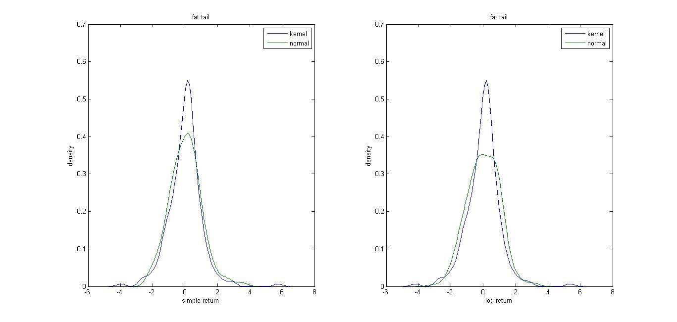
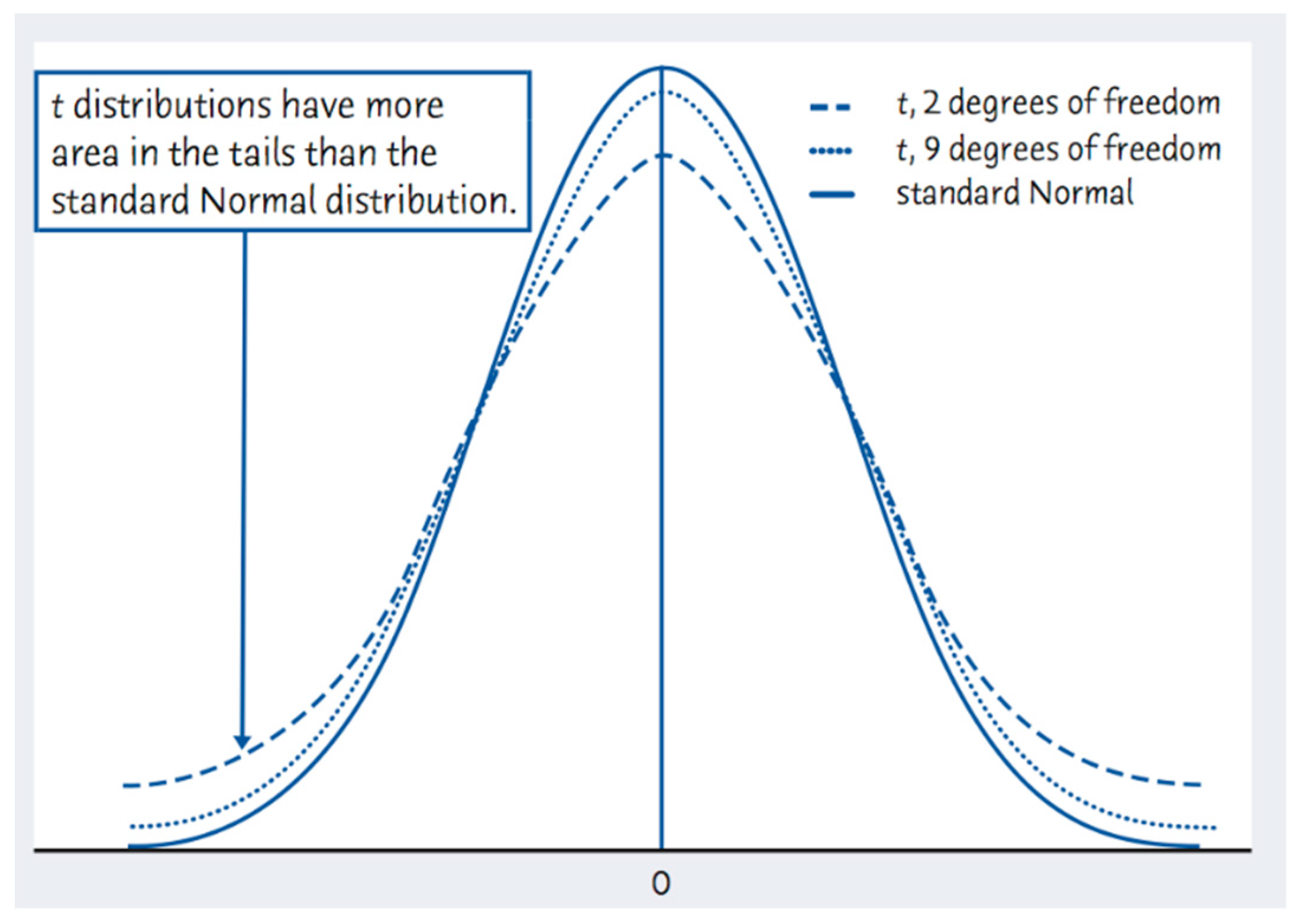
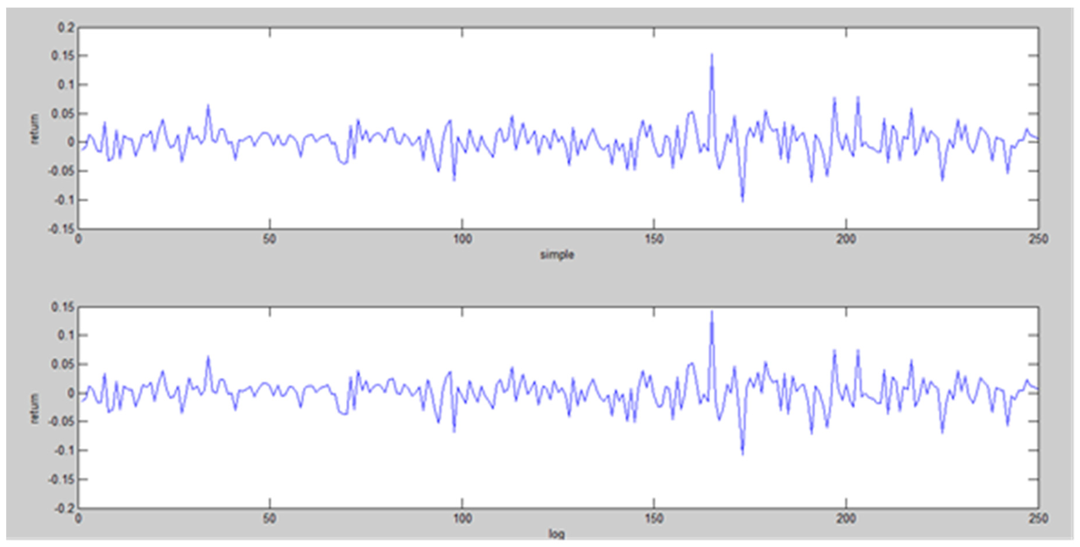
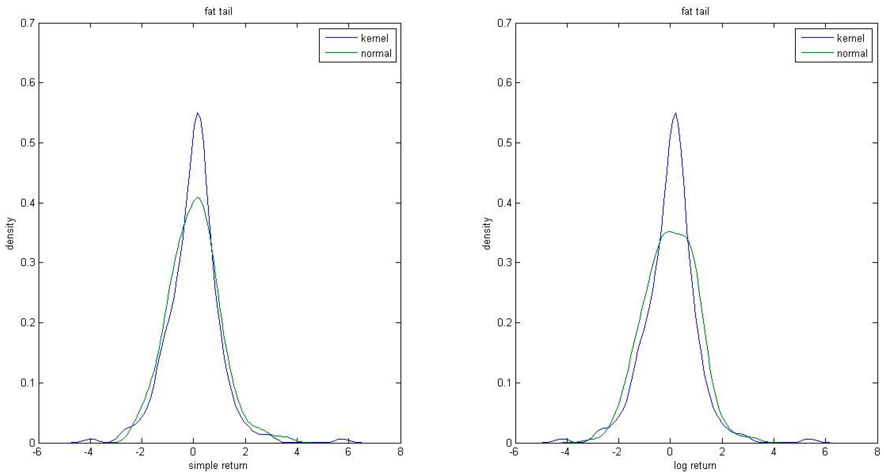
Table 1.
Selected work on Copula.
| Author | Year | Paper/Book/Thesis Title (Please See References for Details) |
|---|---|---|
| Sklar | 1959 | Fonctions derépartitionàn dimensions et leurs marges |
| Joe | 1997 | Multivariate Models and Dependence Concepts |
| Embrechts | 1999 | An Introduction to Copulas |
| Mashal and Zeevi | 2002 | Beyond correlation: Extreme co-movements between financial assets |
| Van den Goorbergh et al. | 2005 | Bivariate option pricing using dynamic copula models |
| Kole et al. | 2007 | Selecting Copulas for risk management |
| Hafner and Reznikova | 2010 | Efficient estimation of a semiparametric dynamic copula model |
Table 2.
Selected works on Portfolio Selection.
| Author | Year | Paper/Book/Thesis Title (Please See References for Details) |
|---|---|---|
| Markowitz | 1952 | Portfolio Selection |
| Samuelson | 1969 | Lifetime portfolio selection by dynamic stochastic programming |
| Merton | 1969 | Life time portfolio selection under uncertainty: The continuous-time case |
| Pogue | 1970 | An extension of the Markowitz portfolio selection model to include variable transactions’ costs, short sales, leverage policies and taxes |
| Merton | 1972 | An analytic derivation of the efficient portfolio frontier |
| Fernández and Gómez | 2007 | Portfolio selection using neural networks |
Table 3.
Selected work on Correlation/Covariance and GARCH.
| Author | Year | Paper/Book/Thesis Title (Please See References for Details) |
|---|---|---|
| Engle | 1982 | Autoregressive conditional heteroscedasticity and estimates of UK inflation |
| Engle et al. | 1984 | Combining competing forecasts of inflation using a bivariate ARCH model |
| Bollerslev | 1986 | Generalized autoregressive conditional heteroscedasticity |
| Bollerslev et al. | 1988 | A capital asset pricing model with time-varying covariances |
| Bollerslev | 1990 | Modelling the coherence in short-run nominal exchange rates: A multivariate generalized ARCH model |
| Engle and Kroner | 1995 | Multivariate simultaneous generalized ARCH |
| Tse and Tsui | 2002 | A multivariate generalized autoregressive conditional heteroscedasticity model with time-varying correlations |
| Engle | 2002 | Dynamic conditional correlation: A simple class of multivariate generalized autoregressive conditional heteroskedasticity models |
| McAleer et al. | 2008 | Generalized autoregressive conditional correlation |
Table 4.
Selected work on Portfolio Selection and VaR/CVaR.
| Author | Year | Paper/Book/Thesis Title (Please See References for Details) |
|---|---|---|
| Baumol | 1952 | The transactions demand for cash: An inventory theoretic approach |
| Goldfarb and Iyengar | 2003 | Robust portfolio selection problems |
| McKay and Keefer | 1996 | VaR Is a Dangerous Technique |
| Artzner et al. | 1997 | Thinking coherently |
| Pflug | 2000 | Some remarks on the value-at-risk and the conditional value-at-risk |
| Uryasev | 2000 | Optimization of Conditional Value-at-Risk |
| Chen and Yang | 2017 | Multiperiod portfolio investment using stochastic programming with conditional value at risk |
| Zhang and Gao | 2017 | Portfolio selection based on a benchmark process with dynamic value-at-risk constraints |
Table 5.
Selected work on Portfolio Selection and Semi variance.
| Author | Year | Paper/Book/Thesis Title (Please See References for Details) |
|---|---|---|
| Roy | 1952 | Safety First and the Holding of Assets |
| Markowitz | 1959 | Portfolio selection: Efficient diversification of investments |
| Bawa and Lindenberg | 1977 | Capital market equilibrium in a mean-lower partial moment framework |
| Bawa | 1978 | Safety-first, stochastic dominance, and optimal portfolio choice |
| Chen et al. | 1991 | A Method for Approximating Semivariance in Project Portfolio Analysis |
| Hamza and Janssen | 1998 | The mean-semivariances approach to realistic portfolio optimization subject to transaction costs |
| Ballestero | 2005 | Mean-semivariance efficient frontier: A downside risk model for portfolio selection |
| Huang | 2008 | Mean-semi variance models for fuzzy portfolio selection |
| Sayilgan and Mut | 2010 | Uses of Variance and Lower Partial Moment Measures for Portfolio Optimization |
© 2019 by the authors. Licensee MDPI, Basel, Switzerland. This article is an open access article distributed under the terms and conditions of the Creative Commons Attribution (CC BY) license (http://creativecommons.org/licenses/by/4.0/).
Share and Cite
MDPI and ACS Style
Sun, R.; Ma, T.; Liu, S.; Sathye, M. Improved Covariance Matrix Estimation for Portfolio Risk Measurement: A Review. J. Risk Financial Manag. 2019, 12, 48. https://0-doi-org.brum.beds.ac.uk/10.3390/jrfm12010048
AMA Style
Sun R, Ma T, Liu S, Sathye M. Improved Covariance Matrix Estimation for Portfolio Risk Measurement: A Review. Journal of Risk and Financial Management. 2019; 12(1):48. https://0-doi-org.brum.beds.ac.uk/10.3390/jrfm12010048
Chicago/Turabian StyleSun, Ruili, Tiefeng Ma, Shuangzhe Liu, and Milind Sathye. 2019. "Improved Covariance Matrix Estimation for Portfolio Risk Measurement: A Review" Journal of Risk and Financial Management 12, no. 1: 48. https://0-doi-org.brum.beds.ac.uk/10.3390/jrfm12010048