Article

Neural Network Predictive Modeling on Dynamic Portfolio Management—A Simulation-Based Portfolio Optimization Approach

Department of Systems Engineering and Operations Research, George Mason University, Fairfax, VA 22030, USA
*
Author to whom correspondence should be addressed.
J. Risk Financial Manag. 2020, 13(11), 285; https://0-doi-org.brum.beds.ac.uk/10.3390/jrfm13110285
Submission received: 9 October 2020 / Revised: 5 November 2020 / Accepted: 13 November 2020 / Published: 17 November 2020
(This article belongs to the Special Issue Artificial Neural Networks in Business)

Abstract

:
Portfolio optimization and quantitative risk management have been studied extensively since the 1990s and began to attract even more attention after the 2008 financial crisis. This disastrous occurrence propelled portfolio managers to reevaluate and mitigate the risk and return trade-off in building their clients’ portfolios. The advancement of machine-learning algorithms and computing resources helps portfolio managers explore rich information by incorporating macroeconomic conditions into their investment strategies and optimizing their portfolio performance in a timely manner. In this paper, we present a simulation-based approach by fusing a number of macroeconomic factors using Neural Networks (NN) to build an Economic Factor-based Predictive Model (EFPM). Then, we combine it with the Copula-GARCH simulation model and the Mean-Conditional Value at Risk (Mean-CVaR) framework to derive an optimal portfolio comprised of six index funds. Empirical tests on the resulting portfolio are conducted on an out-of-sample dataset utilizing a rolling-horizon approach. Finally, we compare its performance against three benchmark portfolios over a period of almost twelve years (01/2007–11/2019). The results indicate that the proposed EFPM-based asset allocation strategy outperforms the three alternatives on many common metrics, including annualized return, volatility, Sharpe ratio, maximum drawdown, and 99% CVaR.

1. Introduction

Markowitz 1952 pioneered the construction of an optimal portfolio by proposing a Mean-Variance model, which created an efficient frontier to model a portfolio’s risk and return trade-off. This laid the foundation for a continuous development of Modern Portfolio Theory (MPT)—a mathematical framework for assembling and allocating a portfolio of assets (equities and bonds are the most common asset classes) with the goal of either maximizing its expected return for a given risk constraint or minimizing its risk for a given expected return constraint. However, a major shortcoming in using variance as a measure of risk is that it cannot measure the tail risk reliably. Realizing this, (Morgan 1996) proposed a concept called Value-at-Risk (VaR), which summarized the worst loss over a target horizon at a determined confidence level. Financial regulators and portfolio managers usually choose 99% as an appropriate confidence level for stress testing and portfolio hedging purposes. Since VaR is easy to calculate, it has been widely accepted in the financial world as a main metric for evaluating downside risk. Besides operational risk, VaR also has applications in the market risk and credit risk domains (see (Dias 2013), (Embrechts and Hofert 2014) for more details). However, due to the fact that VaR is neither subadditive nor convex, and that the distribution of real-world financial asset returns data is found to exhibit substantial heavy tails and asymmetry around the mean (see (Shaik and Maheswaran 2019)), (Artzner et al. 1999) proved that VaR is not a coherent measure of risk for asymmetric distribution.
To overcome the above shortcomings of VaR, (Rockafellar and Uryasev 2002) and (Rockafellar and Uryasev 2000) suggested an alternative metric, known as Conditional Value-at-Risk (CVaR) or Expected Shortfall (ES). This metric is used to measure the expected loss amount exceeding a given VaR. Since CVaR inherits most properties of VaR, it accounts for the severity of the losses and satisfies the subadditivity and convexity properties, which enables CVaR to characterize tail distributions and estimate risk of assets more accurately. In 2000, R.T. Rockafellar et al. showed that for non-normal and non-symmetric distributions, these two frameworks revealed significant differences, and were heavily dataset-specific, as shown in (Krokhmal et al. 2001) and (Larsen et al. 2002). As CVaR only measures the downside risk, it captures both the asymmetric risk preferences of investors as well as the incidence of ”fat” left tails induced by skewed and leptokurtic return distributions, judged by major institutional investors (Sheikh and Qiao 2009) as one of the most appropriate risk measures. Due to these reasons, we choose CVaR as the risk measure and propose a Mean-CVaR framework for portfolio optimization. In addition, since the return series of most asset classes exhibit leptokurtosis, heavy tails, volatility clustering, and interdependence structures, relying solely on the historical return series with Mean-CVaR would skew the optimal asset allocations. Therefore, we propose employing a pair copula-GARCH model for capturing both the volatility clustering and interdependence characteristics in the investment universe.
Finally, in order to capture the impact and benefits from macroeconomy down to the real investment asset classes, we select a number of important economic variables and build an economic factors-based predictive model to learn this relationship. The proposed Economic Factor-based Model (EFPM) uses the pair copula generalized autoregressive conditional heteroskedasticity (GARCH) technique to simulate macroeconomic variables and feed them into a neural network model to generate return series for a list of investment assets. The simulated returns are then fed into a Mean-CVaR framework to obtain the optimal portfolio allocation. Finally, a rolling basis out-of-sample empirical test is conducted to compare the performance of the resulting portfolio against three alternative benchmarks: equally weighted (EW), historical return-based (HRB), and direct simulation (DS) approaches.
Traditional portfolio optimization is performed either under historical return or direct simulation of a series of financial assets based on the learned characteristics of time series. Recent research has begusn to utilize various artificial intelligence and machine-learning techniques in asset pricing and market trend predictions to improve profitability. (Chang et al. 2012) proposed a new type of neural network (involving partially connected architecture) to predict stock price trends from technical indicators. (Yono et al. 2020) used a supervised latent Dirichlet allocation (sLDA) model to define a new macroeconomic uncertainty index based on text mining for news and supervised signals generated from the VIX index. (Zhang and Hamori 2020) applied random forest, support vector machine, and neural networks to a list of macroeconomic factors, including Producer Price Index (PPI) and Consumer Price Index (CPI), to demonstrate the effectiveness of these methods in predicting foreign exchange rates.
Because existing research on machine learning focuses mainly on the predictivity of a variety of factors for market trends or certain indices, there was not much literature on the simulation of investment assets based on information learned through macroeconomic factors. In this paper, we propose to first model the relationship between temporally correlated macroeconomic variables and a set of investment assets with a feedforward artificial neural network. At the same time, we combine copula dependence structure with the GARCH(1,1) framework to model and learn the volatility structure of the macroeconomic factors. The resulting models are used to simulate a large number of macroeconomic samples as input to feed into the trained neural network. The neural network fuses the macroeconomic factor samples and maps them onto the investment returns to be used to derive optimal asset allocation. We demonstrate the effectiveness of this novel approach against other alternatives over several key performance metrics.
The remainder of this paper is organized as follows. Section 2 introduces GARCH framework to model time varying volatility, pair copula construction for dependence structure, and Mean-CVaR optimization process. The neural network model is then proposed in Section 3 to estimate the relationship between a list of macroeconomics and returns for the investment assets, which leads a novel simulation-based portfolio optimization technique. Section 4 documents the empirical results, and Section 5 summarizes our findings.

2. Mathematical Definition and Preliminaries

In this section, we will go over some key concepts and their mathematical characteristics used in this simulation-based portfolio optimization framework. Section 2.1 reviews time-varying volatility and the classical GARCH model as well as its procedure to generate simulated returns for each investment asset class. Section 2.2 further utilizes the Copula concept to enhance the GARCH model to take into account the nonlinear relationships within each investment. Section 2.3 presents the traditional portfolio optimization frameworks using Mean-Variance, Mean-VaR, and lastly Mean-CVaR. It describes the objective, constraints of the optimization problems and ways to solve them.

2.1. Time-Varying Volatility

One important measure in the financial management area is the risk metric, which is usually gauged by volatility or standard deviation of return series of investment assets over a certain period of time. Estimation or prediction of investment assets’ volatility then becomes necessary and vital during portfolio optimization and risk management. Two of the most classic models of volatilities are the so-called ARCH (autoregressive conditional heteroskedastic) introduced by (Engle 1982) and GARCH (generalized autoregressive conditional heteroskedastic) models from (Engle and Bollerslev 1986) and (Taylor 1987). Let us first review some basic concepts.
Denote P i , t as the month end price for an investment asset or economics indicator. Thus, the log return R t can be expressed as the log-percentage change below:
R t = log ( P t ) log ( P t 1 )
R t is final time series with mean μ and volatility σ t with the assumption that volatility varies over time. The return series of assets observed across different financial markets all share some common factors known as “stylized empirical facts.” These facts include the following properties:
  • Heavy Tails: the distribution of returns usually shows a power-law or Pareto-like tail index with a value between two to five for most financial data.
  • Gain or Loss Asymmetry: large drawdowns in stock prices or index do not necessarily reflect equally large upward movements.
  • Volatility Clustering: different measures of volatility tend to have positive correlation over multiple trading periods, which reveals the fact that high-volatility events tend to cluster over time.
In order to capture the time-varying and clustering effects of the volatility, we first introduce ARCH model assuming return of investment assets or economics indicator is given by:
R t = μ + ϵ t
An ARCH ( p ) process is given by
ϵ t = σ t z t
σ t 2 = ω +   i = 1 p α i ϵ t i 2  
where { z t } is a sequence of white noise with mean 0 and variance 1, and ω > 0 , α i 0 ,     i = 1 , ,   p . In this article, we assume { z t } follows a skewed generalized error distribution (SGED), which was introduced by (Theodossiou 2015) to accommodate skewness and leptokurtosis to the generalized error distribution (GED). The probability density function (PDF) for SGED is as follows:
f y = k 1 1 k 2 φ Γ ( 1 k ) 1 exp ( 1 k | μ | k ( 1 + s g n ( μ ) λ ) k φ k )
where u = y m , m is the mode of the random variable y , φ is a scaling constant related to the standard deviation of y , λ is a skewness parameter, k is a kurtosis parameter, s g n is the sign function of −1 for u < 0 and 1 for u > 0 and Γ ( · ) is gamma function.
For simplicity’s sake, given p = 1 , we have ARCH(1) process and error term ϵ t with conditional mean and conditional variance as follows:
E ( ϵ t | ϵ t 1 ) = E ( σ t z t | ϵ t 1 ) = σ t E ( z t | ϵ t 1 ) = σ t E ( z t ) = 0
V a r ( ϵ t | ϵ t 1 ) = E ( σ t 2 z t 2 | ϵ t 1 ) = σ t 2 E ( z t 2 | ϵ t 1 ) = σ t 2 E ( z t 2 ) = σ t 2 1 = σ t 2
and unconditional variance of ϵ t is
V a r ( ϵ t ) = E ( ϵ t 2 ) ( E ( ϵ t ) ) 2 = E ( ϵ t 2 ) = E ( σ t 2 ) = ω + α 1 E ( ϵ t 1 2 ) = ω 1 α 1
since ϵ t is a stationary process and V a r ( ϵ t ) = V a r ( ϵ t 1 ) = E ( ϵ t 1 2 ) .
As the extension to include flexible lag terms for ARCH model, GARCH ( p , q ) model considers the same stochastic process defined under Equation (3) and introduces an additional lagged q -period conditional variance term within the formulation of conditional variance:
ϵ t = σ t z t σ t 2 = ω + i = 1 p α i ϵ t i 2 + j = 1 q β j σ t j 2
where ω > 0 ,   α i , β j 0 . The simplest and most widely used version for GARCH ( p , q ) model is GARCH(1,1):
ϵ t = σ t z t σ t 2 = ω + α 1 ϵ t 1 2 + β 1 σ t 1 2
It can be shown that the above has a stationary solution with a finite expected value if and only if α 1 + β 1 < 1 and its long run variance is V L = E ( σ t 2 ) = ω 1 α 1 β 1 . Thus GARCH(1,1) can be rewritten as
ϵ t = σ t z t σ t 2 = γ V L + α 1 ϵ t 1 2 + β 1 σ t 1 2

2.2. Dependence Modeling and Pair Copula

There is a large body of research articles that indicate that conditional volatility of economic time series varies over time. Researchers then proposed the copula technique, which allows us to model a dependence structure independent of multivariate distribution. (Sklar 1959) first proposed copula to measure nonlinear interdependence between variables. Then, (Jondeau and Rockinger 2006) proposed the copula-GARCH model and applied it to extract the dependence structure between financial assets. Copula plays a vital role in financial management and econometrics and is widely used on Wall Street to model and price various structured products, including Collateralized Debt Obligations (CDOs). The key contribution of copula is to separate the marginal distribution from the dependence structure and improve the correlation definition from linear to also considering nonlinear relationships.
In a review article from (Patton 2012), he defined a n-dimensional copula assuming Y = ( Y 1 , ,   Y n   ) T as random vector with cumulative distribution function F and for i { 1 , ,   n } , letting F i denote the marginal distribution of Y i , thus there exists a copula C : [ 0 , 1 ] n [ 0 , 1 ] such that for all y = ( y 1 , ,   y n   ) T n
F ( y ) = C { F 1 ( y 1 ) , ,   F n ( y n ) }
In the application of multivariate time series, Patton used a version of Sklar’s theorem and decomposed the conditional joint distribution given some previous information set into conditional marginal distribution and conditional copula. For t ( 1 , ,   T ) , let Y t | t 1 F ( · | t 1 ) and Y i , t | t 1 F i ( · | t 1 ) then
F ( y | 𝓕 t 1 ) = C { F 1 ( y 1 | 𝓕 t 1 ) , ,   F n ( y n | 𝓕 t 1 ) | 𝓕 t 1 }
From the above section of the GARCH model, we now incorporate Equations (2) and (11) to the multivariate copula, and the white noise term { z t } can be derived from copula structure
z t | t 1 F z t = C t ( F 1 , t , ,   F n , t )
where z t can be estimated from R t μ σ t | t 1 .
As the marginal distributions F i are usually not known or hard to obtain from a parametric approach, here we propose a nonparametric method to estimate them using the empirical distribution function (EDF) introduced by (Patton 2012). For a nonparametric estimate of F i , we use the following function with uniform marginal distribution:
F i ^ ( z ) 1 T + 1 t = 1 T 1 ( z ^ i , t z ) U ^ i , t = F i ^ ( z ^ i , t )
where 1 ( z ^ i , t z ) is the indicator function of 1 when z ^ i , t z .
There are two well-known classes of parametric copula functions, i.e., elliptical family and the Archimedean copula. Gaussian and t -copulas are the two types from the elliptical family where their density functions come from elliptical distribution.
Assume random variable X ~ M N o r m a l ( 0 , P ) where P is the correlation matrix of X . Gaussian copula is defined as:
C P G a u s s = Φ P ( Φ 1 ( u 1 ) , ,   Φ 1 ( u d ) )
where Φ ( · ) is standard normal cumulative distribution function (CDF) and Φ P is the joint CDF for multivariate normal variable X . This copula above is the same for random variable Y ~ M N o r m a l ( μ , Σ ) if Y has the same correlation matrix P as X .
Similar to the Gaussian copula above, if W follows multivariate t -distribution with v degree of freedom and can be written as W = X / ξ v where X ~ M N o r m a l ( 0 ,   Σ ) and ξ ~ χ v 2 independent of v . the t -copula is defined as:
C v , P t = t v , P ( t v 1 ( u 1 ) , ,   t v 1 ( u d ) )
where P is the correlation matrix of W , t v , P is the joint CDF of W and t v is the standard t -distribution with degree of freedom v .
The other important class of copula is the Archimedean copula (Cherubini et al. 2004), which can be created using a function ϕ : I + , continuous, decreasing, convex, and ϕ ( 1 ) = 0 . Such function is called generator, and pseudo-inverse is defined from the generator function as follows:
ϕ [ 1 ] ( v ) = { ϕ 1 ( v )       0 v ϕ ( 0 ) 0                                 ϕ ( 0 ) v
This pseudo-inverse will generate the same result as the normal inverse function as long as it is within the domain and range : ϕ [ 1 ] ( ϕ ( v ) ) = v for every v I . Given the generator and pseudo-inverse, Archimedean copula C A can be generated from the following form:
C A ( v , z ) = ϕ [ 1 ] ( ϕ ( v ) + ϕ ( z ) )
There are two important subclasses of Archimedean copulas that have only one parameter in the generator—Gumbel and Clayton copulas, as given in Table 1.
In practice, the complexity of estimating parameters from multivariate copula increases rapidly when the dimension of time series data expands. Therefore, (Harry 1996), (Bedford and Cooke 2001), (Aas et al. 2009), and (Min and Czado 2010) independently proposed a multivariate probability structure via a simple building block—pair copula construction (PCC) framework. The model decomposes multivariate joint distribution into a series pair copula on different conditional probability distributions with an iterative process. The copula definition from Equation (12) can be rewritten using uniformly distributed marginals U ( 0 , 1 ) , as follows:
C ( u 1 , ,   u n ) = F { F 1 1 ( u 1 ) , ,   F n 1 ( u n ) }
where F i 1 ( u i ) is the inverse distribution function of the marginal. We can then derive the joint probability density function (PDF) f ( · ) as follows:
f ( y ) = c 1 , ,     n   { F 1 ( y 1 ) , ,   F n ( y n ) } · f 1 ( x 1 ) f n ( x n )
for some (uniquely identified) n -variate copula density c 1 n ( · ) with a conditional density function given as,
f ( y | v ) = c y v j | v j   { F ( y | v j ) ,   F ( v j | v j ) } · f ( y | v j )
where for a n -dimensional vector v , v j represents an element from v and v j is the vector without element v j .
Therefore, the multivariate joint density function can be written as a product of pair copula on different conditional distributions. For example, under the bivariate case, the marginal density distribution of y 1 | y 2 can be written using the formula above as,
f ( y 1 | y 2 ) = f ( y 1 , y 2 ) f ( y 2 ) = c 12   { F 1 ( y 1 ) ,   F 2 ( y 2 ) } · f 1 ( y 1 ) · f 2 ( y 2 ) f ( y 2 ) = c 12   { F 1 ( y 1 ) ,   F 2 ( y 2 ) } · f 1 ( y 1 )
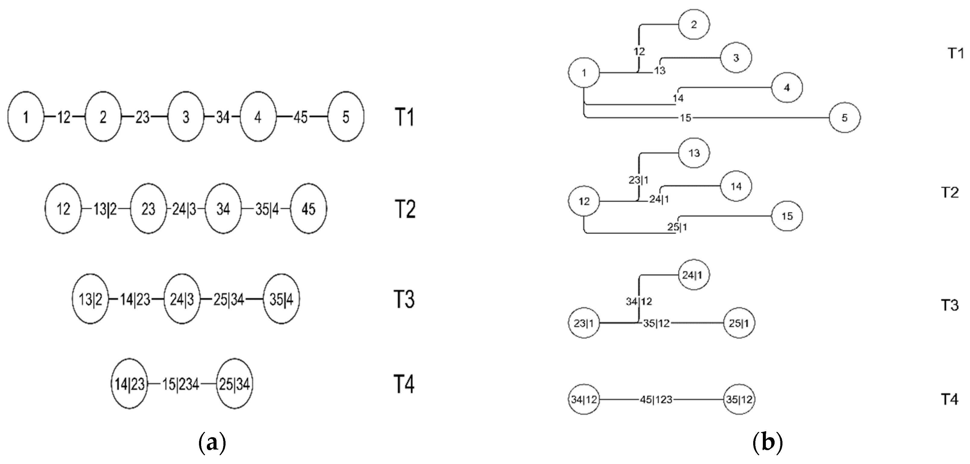
For high-dimension data, there are a large number of combinations for the pair copulas. Therefore, (Bedford and Cooke 2001, 1999) proposed using a graphic approach known as “regular vine” to systematically define the pair copula relationship in the tree structure. Each edge in the vine tree corresponds to a pair copula density. The density of a regular vine distribution is defined by the multiplication of pair copula densities over n ( n 1 ) 2 edges in a regular vine tree structure and the multiplication of the marginal densities. (Aas et al. 2009) and (Kurowicka and Cooke 2007) further introduced canonical vine and D-vine as two special cases of regular vine to decompose the density. Canonical vine distribution is a regular vine distribution but with unique nodes connected to the remaining n j nodes under each tree. In the D-vine structure, no node in any tree can be connected to more than two nodes. The n-dimensional density of canonical vine can be written as follows:
f ( y 1 , ,   y n ) = k = 1 n f ( y k ) j = 1 n 1 i = 1 n j c j , j + i | 1 , ,     j 1 { F ( y j | y 1 , ,   y j 1 ) , F ( y j + i | y 1 , ,   y j 1 ) }
where j denotes the trees and i spans the edge of each tree. The n-dimensional density of D-vine is given as,
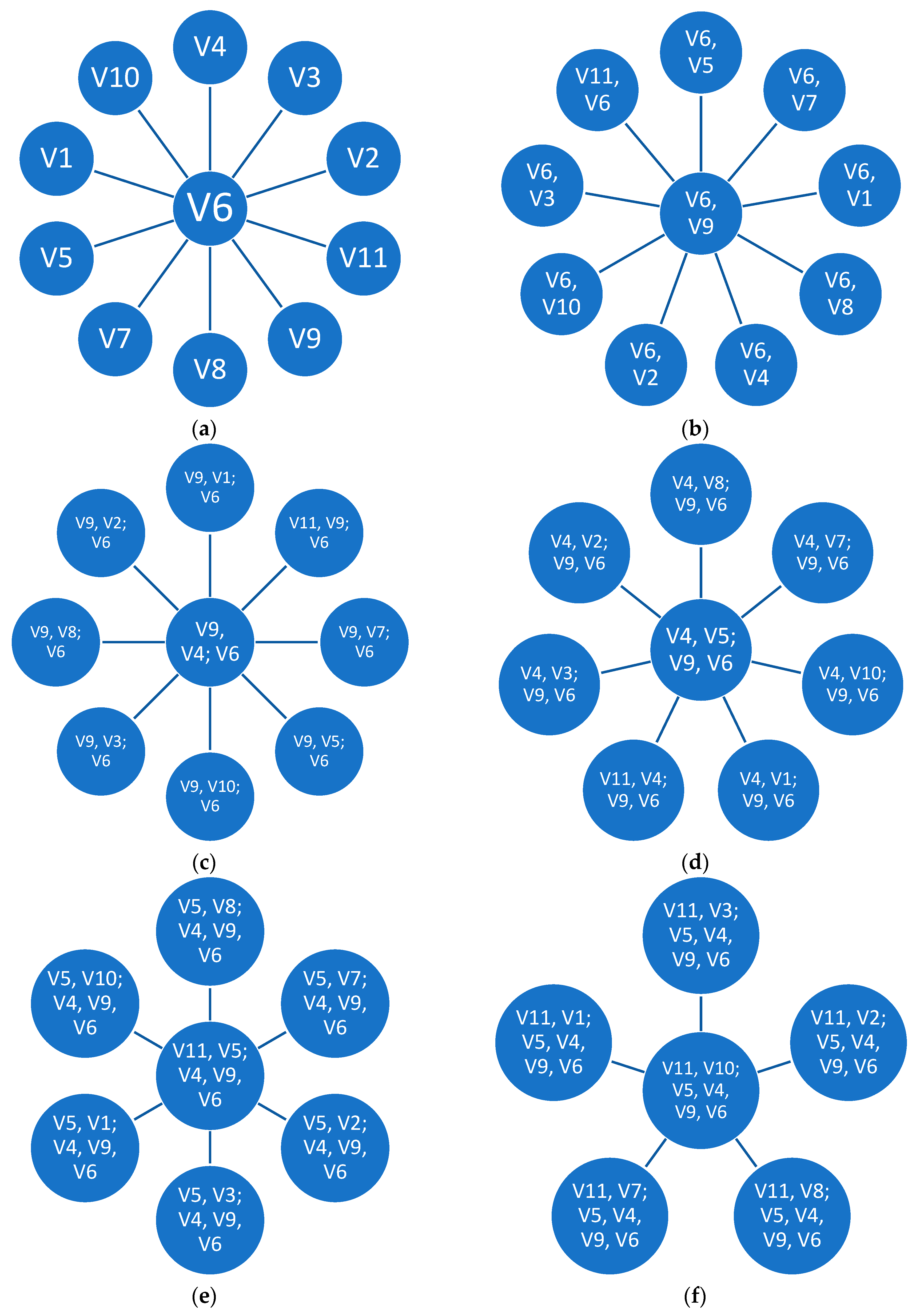
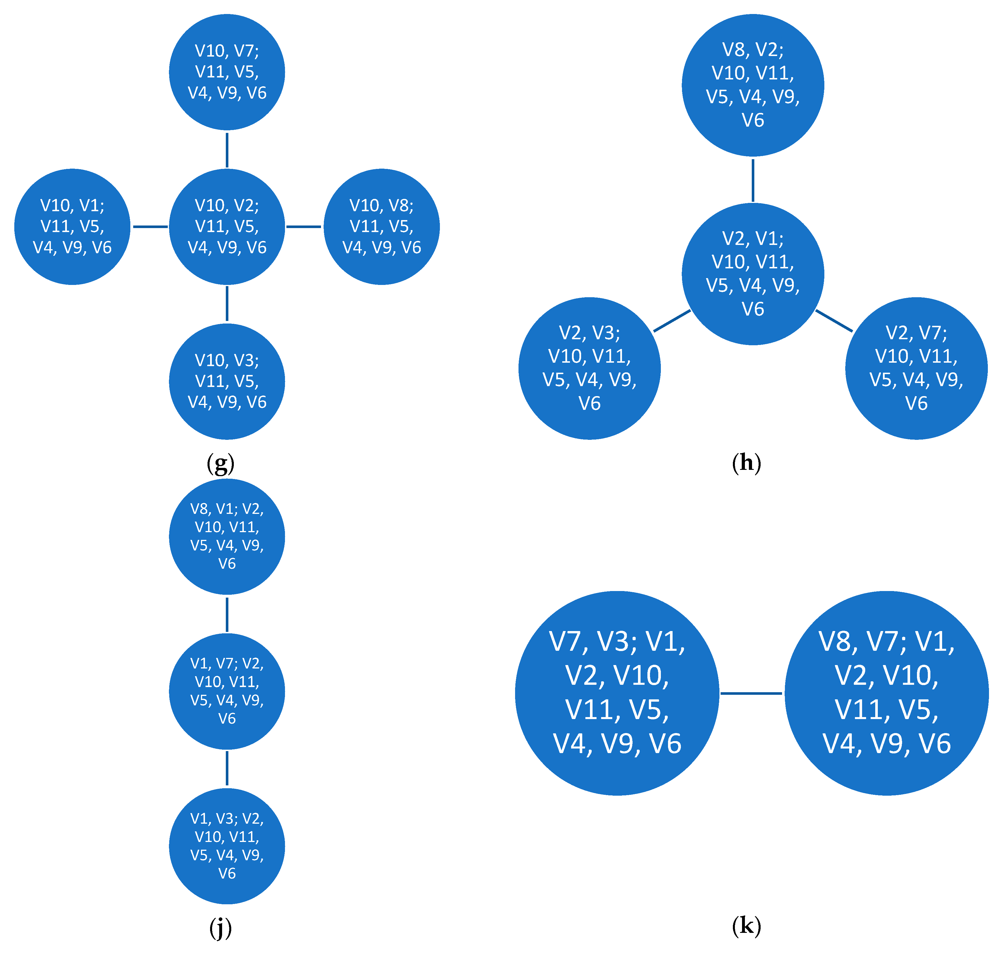
f ( y 1 , ,   y n ) = k = 1 n f ( y k ) j = 1 n 1 i = 1 n j c i , i + j | i + 1 , , i + j 1 { F ( y i | y i + 1 , ,   y i + j 1 ) , F ( y i + j | y i + 1 , ,   y i + j 1 ) }
The chart in Figure 1 shows an example of five variable vine copulas constructed from canonical vine and D-vine structures, respectively.
In this paper, we focus on the canonical vine copula structure. To review the simulation techniques from canonical vine, here are the main steps proposed by (Aas et al. 2009) as shown in Algorithm 1:
Algorithm 1. Simulation algorithm for canonical vine copula.
Generate one sample y 1 ,   ,   y n from canonical vine
  Sample u 1 ,   ,   u n independently from U n i f o r m ( 0 , 1 )
   y 1 = v 1 , 1 = u 1
  for   i 2 , ,   n
    v i , 1 = u i
    for k i 1 , i 2 , 1
      v i , 1 = h 1 ( v i , 1 , v k , k , Θ k , i k )
end for
    y i = v i , 1
    if i = = n then
stop
    end if
    for j 1 , ,   i 1
      v i , j + 1 = h ( v i , j , v j , j ,   Θ j , i j )
    end for
  end for
where function h ( y , v , Θ ) is defined as the marginal conditional distribution function derived from the conditional density defined in Equation (22). Thus, when y and v are uniform, i.e., f ( y ) = f ( v ) = 1 ,   F ( y ) = y ,   F ( v ) = v , h ( y , v , Θ ) has the following form:
h ( y , v , Θ ) = F ( y | v ) = C y , v ( y , v , Θ ) v
where Θ denotes the set of parameters for the copula of the joint distribution function of y and v , further defining h 1 ( y , v , Θ ) as the inverse of the conditional distribution and as the inverse function of h ( · ) with respect to y .
To estimate the parameters of the pair copula, (Aas et al. 2009) proposed using the pseudo-maximum likelihood to estimate parameters sequentially along the multiple layers of pair copula trees. The log-likelihood is given as,
L ( y , v , Θ ) = j = 1 n 1 i = 1 n j t = 1 T log [ c j , j + i | 1 , ,   j 1 { F ( y j , t | y 1 , t , ,   y j 1 , t ) , F ( y j + i , t | y 1 , t , ,   y j 1 , t ) } ] = t = 1 T log ( c ( y t , v t , Θ ) )
where c ( u , v , Θ ) is the density of bivariate copula with parameter Θ .
With the goodness-of-fit test using the Akaike Information Criterion (AIC) metric defined by (Akaike 1998), we can find the copula family that minimizes this metric as the best copula family for each tree.
A I C = 2 t = 1 T log [ c ( y t , v t , Θ ) ] + 2 k
where k is the number of parameters in the model. It is used to penalize the log-likelihood by its complexity. The model selection process involves finding the copula family that minimizes the AIC score.

2.3. Portfolio Optimization Using Mean-CVaR

In this section, we first review the traditional mean-variance portfolio optimization framework proposed by (Markowitz 1952). Then we review another classical risk metric, value-at-risk (VaR), as an alternative to variance. (Rockafellar and Uryasev 2002) and (Rockafellar and Uryasev 2000) extended VaR metrics, which focused on the percentile loss to conditional VaR (CVaR) or expected shortfall as average of the tail loss. We will then focus on portfolio optimization using the mean-CVaR framework.
Given a list of N investment assets, the mean-variance optimization is to find the optimal weights vector w = ( w 1 , w 2 , , w N ) T of those assets so that the portfolio variance is minimized given a specific level of portfolio expected returns. This problem can be written as follows,
min w W                                                     w T Σ w           s . t .                         { i = 1 N w i = 1 w T y μ 0  
where μ = ( y 1 , ,   y N ) T is the return vector for each of the N investment asset classes, Σ is the covariance matrix of the N asset return series, and μ 0 is the minimum expected return of the portfolio.
In this framework, Markowitz combined return with covariance matrix as the risk metric. However, other risk metrics have been introduced to focus on the tail events where losses occur. Value at Risk (VaR) is one of these measures, proposed by (Morgan 1996) for the extreme potential change in value of a portfolio under a given probability over a certain predefined time horizon. In this paper, we focus on an extension of VaR – Conditioned VaR (CVaR), which is defined as the mean loss that exceeds the VaR at some confidence level. Mathematically, VaR and CVaR can be written as follows:
V a R β ( w ) = min { l : Ψ ( w , l ) β } C V a R β ( w ) = 1 1 β f ( w , y ) V a R β ( w ) f ( w , y ) p ( y ) d y
where y represents returns with density p ( y ) and β is the confidence level.
Here we define the loss function as f ( w , y ) = w T y and the corresponding probability of the loss that would not exceed a certain level l can be expressed as Ψ ( w , l ) = f ( w , y ) l p ( y ) d y . Thus, V a R β ( w ) is the VaR and C V a R β ( w ) is the expected loss of the portfolio at the β confidence level. It is clear that C V a R β ( w ) V a R β ( w ) . (Rockafellar and Uryasev 2002) and (Rockafellar and Uryasev 2000) show that CVaR can be derived from the following optimization problem without first calculating VaR:
F β ( w , l ) = l + 1 1 + β f ( w , y ) l [ f ( w , y ) l ] + p ( y ) d y V a R β ( w ) argmin l ( F β ( w , l ) ) C V a R β ( w ) min l F β ( w , l )
where [ f ( w , y ) l ] + = max ( f ( w , y ) l , 0 ) and F β ( w , l ) is a function of l and convex as well as continuously differentiable. Furthermore, the integral part under F β ( w , l ) can be simplified by discretizing based on the density function p ( y ) to a q -dimension sample,
F β ( w , l ) = l + 1 q ( 1 + β ) k = 1 q [ f ( w , y k ) l ] +
Minimizing CVaR as the risk metric is thus equivalent to minimizing F β ( w , l ) from the above formula. To construct the portfolio optimization using CVaR as the risk metric, we can formulate the following problem similar to the Mean-Variance problem above,
min w W                                                     F β ( w , l ) = l + 1 q ( 1 + β ) k = 1 q S k     s . t .                         { S k f ( w , y k ) l = w T y k l S k 0 i = 1 N w i = 1 w T y μ 0  
where S k is an auxiliary term to approximate [ f ( w , y k ) l ] + so that the problem becomes a linear programming problem that can be solved easily and does not depend on any distribution assumption for the return series y k .

3. Neural Net-Based Pair Copula GARCH Portfolio Optimization Framework

In this section, a new approach toward portfolio optimization is proposed using the GARCH and pair copula techniques to generate simulated return series of investment vehicles from a list of economic indicators, which are then fitted into the portfolio optimization framework of Mean-CVaR (presented earlier) to derive the optimal allocation over time.

3.1. Economic Factor-Based Predictive Model (EFPM)

Historically, linear models like AR, ARMA, and ARIMA were used in forecasting stock returns introduced by (Zhang 2003) or (Menon et al. 2016). The problem with these models is that they only work for a particular type of time series data (i.e., the established model may work well for one type of equity or index fund but may not perform well for another). To solve this problem, (Heaton et al. 2017) applied deep learning models for financial forecasting. Deep neural networks (also known as artificial neural networks) are good at forecasting because they can approximate the relationship between input data and predicted outputs, even when the inputs are highly complex and correlated.
Over the past few decades, many researchers have applied various deep learning algorithms for forecasting, such as Recurrent Neural Network (RNN) (Rout et al. 2017), Long short-term memory (LSTM) (Kim and Kim 2019; Nelson et al. 2017), and Convolutional Neural Network (CNN) (Selvin et al. 2017). However, none of these approaches specifically took into account macroeconomic factors in the learning algorithms to predict stock returns. To the extent of our knowledge, very little work was done to explicitly explore hidden information and the relationships between macroeconomic factors and financial asset returns. In this paper, we propose applying a set of well-known and important economic variables (see Appendix A for detailed descriptions) as the input layer and building a feedforward neural network model with one hidden layer and one output layer. Our goal is to construct a predictive model characterizing the relationship between the monthly log-percentage change of macroeconomic variables and the returns of financial investment instruments.
To discover such relationships, we first partition historical monthly log-percentage change for each of the macroeconomic variables and log return series of investment assets into a training set and a test set. The training model for a three-layer neural network is fitted onto the training set and tested on the test set. This process involves tuning the hyperparameter and finding the optimal numbers of hidden neurons that minimize the mean squared error between the predictive value and the actual value.
This artificial neural network takes simulation of economic factors as input and produces returns of investment assets as output. The equation below illustrates the feedforward process of how to map the input data to the output. The learning process is to seek optimal weights w k ,   o u t p u t and w j k that minimize a defined error function,
y ^ i = ϕ o u t p u t ( α l + k o u t p u t w k ,   o u t p u t   ϕ k ( α k + j k w j k x i j ) )
where α is bias term, ϕ is activation function and default to sigmoid function ( e x 1 + e x ) in this paper. The error function is defined as sum of squared error (SSE) between true value and estimated value of output. To find the optimal weights w k ,   o u t p u t and w j k , the learning process uses a gradient descent method to iteratively update w j k based on w j k w j k η S S E w j k ,   where   η is the learning rate that controls how far each step moves in the steepest descent direction. Figure 2 shows an example of such a neural network model constructed based on historical data of economic factors and investment assets, to be introduced in Section 4.

3.2. Return Series Simulation from Pair Copula-GARCH Framework

Once the neural network model is constructed between economic factors and investment assets, we propose generating simulated time series of the monthly log-percentage change from a pair copula-GARCH framework (presented in Section 2). The simulated time series are then fed into the above neural network to generate the simulated return series of investment assets. In this section, we detail the process of simulating the monthly log-percentage change from the pair copula-GARCH framework.
In this paper, we adopt the popular GARCH(1,1) model described in Equation (11) to model the time-dependent volatility. GARCH(1,1) is widely used not only for financial assets but also for macroeconomic variables. (Hansen and Lunde 2005) compared 330 GARCH-type models in terms of their abilities to forecast the one-day-ahead conditional variance for both foreign exchange rate and return series for IBM stock. They concluded that there is no evidence that GARCH(1,1) is outperformed by other models for exchange rate data; however, it is inferior for IBM return. (Yin 2016) applied univariate GARCH(1,1) with macroeconomic data to model uncertainty and oil returns to evaluate whether macroeconomic factors affect oil price. (Fountas and Karanasos 2007) used the univariate GARCH model on inflation and output growth data to test for the causal effect of macroeconomic uncertainty on inflation and output growth and concluded that inflation and output volatility can depress real GDP growth.
As the monthly time series data of macroeconomic variables have both time-varying volatility and nonlinear interdependence structures between their tails, we employ the pair copula-GARCH model to generate simulated log-percentage change of a list of key macroeconomic factors. Algorithm 2 summarizes this simulation process with the model learned from their historical data using the pair copula-GARCH framework.
Algorithm 2. Simulation algorithm for time series of macroeconomic variables.
Generate N sample of Simulated Time Series
  • Compute the monthly log-percentage change of macroeconomic:
R t = log ( P t ) log ( P t 1 )
2.
Fit the error term of monthly log-percentage change minus its average for each macroeconomic variable into the GARCH(1,1) process for time-varying volatility, respectively, based on skewed generalized error distribution (SGED), generalized error distribution (GED), or Skew Student-t Distribution (SSTD) if the distribution fit fails to converge with SGED,
for t 1 ,   2 , ,   T
ϵ i , t 1 = R t 1 μ t
σ ^ i , t 2 = ω + α i , 1 ϵ i , t 1 2 + β i , 1 σ ^ i , t 1 2
end for
3.
Apply the volatility scaled error term R t μ t σ t | t 1 from the GARCH(1,1) result to fit the empirical distribution to obtain the CDF for each economic variable, and then use those to fit the canonical vine copula from a family of Gaussian, t , Gumbel, and Clayton copula using the pair copula construction approach. Simulate N samples u i , j from canonical vine copula above for each economics variable j .
4.
Calculate the quantiles based on the fitted SGED distribution of error terms divided by the volatility for such quantiles to obtain simulated white noise term,
{ z ^ i , T } = F 1 ( u i , j ) σ ( F 1 ( u i , j ) )
5.
Determine the next step log-percentage change from its joint distribution using sample mean between time 1 and time T, last period conditional volatility σ ^ i , T and the simulated white noise z ^ i , T using the following:
R ^ T + 1 = μ 1 : T + σ ^ i , T z ^ i , T  

3.3. Portfolio Optimization under Mean-CVaR Using Simulated Returns

Simulated time series of monthly log-percentage change generated from the pair Copula-GARCH framework are then fed into the trained neural network model to produce return series of investment assets. This process maps the simulated economic factors to return series of investment vehicles through the trained neural network to depict the relationship between economic factors and investment assets. As shown in Algorithm 2, the log-percentage change of economic factors is obtained by adding the historical mean to its error term modeled by pair copula and GARCH(1,1). Economic data usually shows a stronger autocorrelation and thus the estimation of log-percentage change can be enhanced by adding the various lagged terms of log-percentage change to the mean and error terms modeled by the GARCH process. However, the goal here is to emulate investment asset returns, which usually have weaker autocorrelation than economic factors. Moreover, investment returns are typically assumed to follow a random walk process,
log ( P t ) log ( P t 1 ) = μ + ϵ t
where log ( P t ) is log price of asset at time t , log ( P t ) log ( P t 1 ) denotes the one period return of investment assets, and μ is the drift term. As investment returns are transformed indirectly from the simulation of economic factors, we carry over this assumption, modeling the time series of economic factors with a constant mean and time-varying volatility as well as dependency structure modeled by copula GARCH(1,1).
Figure 3 summarizes the high-level model architecture describing the process and data flow from neural network fitting and pair copula-GARCH framework, to the final portfolio optimization. The process consists of four steps:
(1)
Train the neural network with historical economic factors as input layer and the investment asset returns as output layer.
(2)
Learn the pair copula-GARCH model with the historical data from economic factors.
(3)
Simulate a large number of economic factor samples based on the learned copula GARCH model. The samples are fed into the trained neural networks.
(4)
The resulting investment asset return samples from the neural network are used to derive the optimal asset allocation based on mean-CVaR principle.
The workflow process starts with collecting historical price series in monthly precision for both macroeconomic factors and investment assets. We then calculate the log-percentage change in time series for both groups of data, respectively. Log-percentage change of economic factors used to fit a univariate GARCH(1,1) process to model the time-varying volatility. We use pair copula construction to model the tail dependence structure and relationships among those factors. A number of simulated time series are generated for economic factors to combine the time-varying volatility, tail dependence structure, and sample mean together.
We build a feedforward neural network to take historical log percentage from economic factors as input and return series from investment assets as output. This neural network will form the mapping relationship between the factors and investment returns. Data for both input and output are derived from the same time horizon. This is analogues-to-factor analysis, which builds a regression-based model to explain the investment returns with a number of fundamental factors. By a similar logic, this process utilizes the machine-learning technique to depict such potentially nonlinear relationships.
Simulated log-percentage changes of economic factors are then fed into trained neural network models to map them into a series of investment asset returns. As the simulation of economic factors stem from the copula GARCH(1,1) model, the resulting investment returns would inherit their characteristics of time-varying volatility, dependence structure, and constant mean of the series. Portfolio optimization system takes the resulting investment returns as the input to derive the optimal weight to be implemented for the next allocation period. This process is repeated for each of the investment cycles.

4. Empirical Exploration and Out-of-Sample Test

In this section, we apply Economic Factor-Based Predictive Model (EFPM) to a list of major economic factors and mutual funds to test the performance of the resulting portfolios on a rolling out-of-sample basis.

4.1. Data Collecction

To compare different portfolio optimization approaches, we chose six Vanguard index mutual funds as the underlying investment instruments and 11 major economic indicators. These index funds range from large-cap and small-cap (based on the company’s market capitalization) equities in the U.S., developed and emerging markets, as well as U.S. real estate and fixed income markets (see Table 2).
These six funds are all tradeable securities with a low expense ratio and relatively longer price history, which makes it easier for us to back-test the model. Using Yahoo! Finance, we collected historical price data for each fund for nearly seventeen years of data between January 2002 and November 2019. Each data point contains information such as daily opening, high, low, close, and adjusted close prices. From these data sets, we extracted only the adjusted close prices at the end of each month and treated them as the proxy of monthly price series. The price histories are plotted in Figure 4 for each index fund.
Furthermore, we apply 11 major macroeconomic variables (with the same time horizon as the index funds, with monthly time series data from January 2002 to November 2019) that reflect most economic activities in the U.S., including money supply, banking, employment rate, gross production, and prices from different aspects of the economy. These key variables depict a holistic picture of the current economic environment and may have predictive power regarding the future trend of investment vehicles. The detailed descriptions of these 11 macroeconomic variables are shown in Appendix A.

4.2. Training and Testing Procedure

Following the process diagram in Section 3.2, we define the model training period as a 60-month interval to learn the optimal weight of six index funds and test out-of-sample data for the following month. The strategy is to capture the short-term momentum and the relatively longer-term mean reversion effects. Thus, the data points in the training and out-of-sample testing are selected to create a balance of meaningful data size, in order to extract such information and appropriate horizons to capture useful market signals. We tested different training period durations, between 36 months to 180 months, and determined that 60 months’ horizon appears to be a reasonable balance of capturing the most recent signals while mining a sufficient pool of historical data. Although there are only 60 data points in the training period to fit the neural network and learn the model, the data samples are displayed in a monthly cycle rather than a daily cycle. (Krämer and Azamo 2007) argued that upward tendency in estimated persistence of a GARCH(1,1) model is due to an increase in calendar time, not to an increase in sample size; therefore, increasing time horizon in the training sample has a better incremental effect of estimating a GARCH(1,1) model than increasing the sample size itself.
This process of 60 months of training and one month out-of-sample testing is repeated on a rolling basis starting from January 2002 and continuing until the last data point in the sample. For each training period, we start with normalizing our training data set so that all the data are within a common range. For this purpose, we utilize min–max normalization method on both the monthly log returns of the six index funds and the monthly log-percentage change of the 11 macroeconomic variables. This normalization tends to accelerate the gradient decent algorithm in the neural network fitting based on (Ioffe and Szegedy 2015).
For each time period, the testing data set is also normalized in the same manner before being fed into the Economic Factor-Based Predictive Model (EFPM). As described earlier, EFPM is a neural network-based model that takes an input of 60-month log-percentage change of 11 macroeconomic variables and generates return series for six index funds of the same time horizon. In the training period, the neural network model further splits this 60-month data set into one training set containing 54 data points to form the model, and the remaining 6-month data that is used to tune the hyperparameter, such as number of neurons in the hidden layer. To measure the error in predicted output during this training period, we employ mean squared error (MSE) metric and select the best network structure that minimizes the MSE,
M S E = 1 n i = 1 n ( P r e d i c t e d i A c t u a l i ) 2
where A c t u a l i stands for the actual i -th monthly log-percentage change, and P r e d i c t e d i represents predicted values given by EFPM.
This relationship between economics variables and index funds is used to transform the simulated log-percentage change of economic variables into simulated return series. Simulation of log-percentage change of economic variables is based on the pair copula-GARCH approach discussed earlier. See Appendix B for sample pair copula constructions fitted using log-percentage change of economic variables. As the output of this process, there are 5000 simulated log-percentage change data points generated from this model. The data is fed into the neural network model to generate 5000 simulated returns data for the six index funds.
Those simulated return series for investment assets are used as input in the Mean-CVaR optimization to find out the optimal weights of the portfolio for the next month. In the optimization, we set confidence level parameter β of CVaR at 99%, and the investor’s expected return parameter μ 0 is set as the minimum of 10% (annualized return) and the average return of the past 60 months among the six investment asset classes.
Portfolio performance for the one-month period is recorded, and this process is repeated the next month using the previous 60 months data again, to construct an optimal portfolio invested for the following month. The rolling out-of-sample test stops when there is no further data available to compute portfolio performance using the optimal weights.
Finally, we compare the entire period of out-of-sample performance using EFPM-based strategy against the three alternative benchmark methods described below,
  • Equally weighted (EW): index funds in the portfolio are simply allocated equally and rebalanced to equal weights each month.
  • Historical return-based (HRB): historical monthly log returns of the six index funds are computed directly as inputs to the Mean-CVaR framework. No simulation is performed here.
  • Direct simulation (DS): monthly log returns of the six index funds are simulated by applying historical data into the pair copula-GARCH framework without utilizing the neural network framework and information from 11 major economic variables.

4.3. Computational Results and Discussions

With the proposed EFPM model and three benchmarks above, there are a total of 154 months of out-of-sample returns. Those returns range from February 2007 to November 2019. To compare the performance for those strategies, we assume $1000 invested at the end of January 2007 to implement the four strategies and rebalance them monthly based on the optimal weights generated.
The investment performance for the four strategies are shown in Figure 5; Figure 6 shows the corresponding optimal allocations for EFPM strategy over time.
Finally, for comparison purposes, we evaluate the performance of the four strategies by looking at the summary statistics to gauge their returns and risks. The metrics we choose include annualized return, annualized volatility, Sharpe ratio, maximum draw-down, and 99% CVaR of all four strategies during the same time period to compare their effectiveness. Results are summarized in Table 3 below:
The results above show that this proposed strategy of embedding the neural network with economic factors to simulate the investment return did outperform the direct simulation using pair copula-GARCH framework on the risk-adjusted return basis. This indicates that there is some explorable information and predictive power in looking at macroeconomic data when simulating return series for these investment vehicles.

5. Conclusions and Future Work

A large body of research has been focused on the school of GARCH models and the conditional dependence structure from copulas. After Jondeau et al. proposed to estimate joint distribution by combining conditional dependency from copulas in the GARCH context in (Jondeau and Rockinger 2006), many researchers have conducted studies utilizing this framework in the field of conditional asset allocation and risk assessment (Wang et al. 2010) in non-normal settings. Meanwhile, with the uptick in research and advancement of modeling and computational efficiency within artificial intelligence and machine learning, these techniques have emerged as a potential tool in analyzing financial market and optimizing investment strategy. Machine learning in this field has mainly focused on predictability of market trend ((Sezer et al. 2017) and (Troiano et al. 2018)), risk assessment ((Chen et al. 2016) and (Kirkos et al. 2007)), portfolio management ((Aggarwal and Aggarwal 2017) and (Heaton et al. 2017)), and pricing for exotics and cryptocurrency.
In this paper, we propose a simulation-based approach for the portfolio optimization problem under the Mean-CVaR framework. This paper proposes to merge and fuse together the two well-established techniques of GARCH framework and machine learning in the application of asset allocation. In order to nudge simulation of investment return to include more market sentiment from a macroeconomics prospective, we build neural networks to model the relationship between macroeconomic time series and the investment asset returns. The time series of economic variables are simulated using pairwise copula-GARCH framework to capture both effects of time-varying volatility and the dependence structure based on historical data. Simulations are then translated through the neural network model to find return series of the final investment assets. Those return series are used to derive optimal allocation via the Mean-CVaR optimization approach. The out-of-sample test result for this model outperformed all the benchmarks created without embedding the macroeconomic information through the neural network.
As our proposed strategy assumes that portfolios incur no transaction cost and employ a “long-only” strategy, future research should consider slippage and trading costs and possibly adopt short-selling and leveraging strategies to reflect real-world scenarios. Also, since it is likely that there exists a causal relationship between the selected macroeconomic variables and index funds’ returns, rather than building the deterministic predictive model utilizing neural network for the selected index funds, future researchers may employ a Bayesian modeling framework (for example, the Black–-Litterman model proposed by (Black and Litterman 1992), or its modified version with the Bayesian framework proposed by (Andrei and Hsu 2018)) to build a stochastic predictive model. This approach may pose some advantages over the former one by incorporating the uncertainty information related to economic factors into the model. As a result, it could lead to better asset allocation for portfolios in a dynamic financial market environment.
With access to various deep neural network and other machine-learning techniques focusing specifically on time series data such as RNN and LSTM, future research can leverage such advanced methods to expand the input layer of the universe of macroeconomic factors and the output layer of investment asset classes, as well as build a deeper hidden layer to search for more trading opportunities for a dynamically managed portfolio.

Author Contributions

Conceptualization, J.Y. and K.-C.C.; methodology, J.Y. and K.-C.C.; software, J.Y.; validation, J.Y. and K.-C.C.; formal analysis, J.Y. and K.-C.C.; investigation, J.Y. and K.-C.C.; resources, J.Y. and K.-C.C.; data curation, J.Y.; writing—original draft preparation, J.Y. and K.-C.C.; writing—review and editing, J.Y. and K.-C.C.; visualization, J.Y. and K.-C.C.; supervision, K.-C.C.; project administration, J.Y. and K.-C.C. All authors have read and agreed to the published version of the manuscript.

Funding

This research received no external funding.

Conflicts of Interest

The authors declare no conflict of interest.

Appendix A. Description of 11 Major Economic Indicators

In this paper, we selected 11 major economic indicators from the Economic Research at Federal Reserve Bank of St. Louis. The Table A1 shows the detailed description for each indicator:
Table A1. List of 11 major macro-economic variables and their descriptions.
Macroeconomic VariablesDescription
University of Michigan: Inflation Expectation1Median expected price change next 12 months.
Consumer Price Index for All Urban Consumers2Average monthly change in the price for goods and services between any two time periods.
S&P/Case-Shiller U.S. National Home Price Index3A leading measure of U.S. residential real estate prices
Crude Oil Prices: West Texas Intermediate (WTI)4Serves as a reference for pricing a number of other crude streams.
Producer Price Index (PPI) for All Commodities5Measures the average change over time in the selling prices received by domestic producers
Import Price Index (End Use): All commodities6Contains data on changes in the prices of goods and services traded between the U.S. and other countries
Export Price Index (End Use): All commodities7Contains data on changes in the prices of goods and services traded between the U.S. and other countries
Trade Weighted U.S. Dollar Index8A weighted average of the foreign exchange value of the U.S. dollar against the currencies of major U.S. trading partners.
3 Month Treasury Bill: Secondary Market Rate9Yields in percent per annum.
Personal Saving Rate10Percentage of disposable personal income (DPI) as the ratio of personal saving to DPI.
1-Month London Interbank Offered Rate (LIBOR)11Average interest rate at which leading banks borrow funds from other banks in the London market.

Appendix B. Sample Pair Copula Constructions

When simulating log-percentage changes from 11 major economic variables, we use pair copula construction to discover the relationship among those variables. Figure A1 is a sample of pair copula trees generated using 60 monthly time series from February 2002 to January 2007.
Figure A1. Pair copula construction on 60 monthly log-percentage change of 11 economic variables starting February 2002: (ak) indicate economic optimal tree structures fitted into the copula family of Gaussian, t, Gumbel, and Clayton.
Jrfm 13 00285 g0a1aJrfm 13 00285 g0a1b

References

  1. Aas, Kjersti, Claudia Czado, Arnoldo Frigessi, and Henrik Bakken. 2009. Pair-Copula Constructions of Multiple Dependence. Insurance, Mathematics & Economics 44: 182–98. [Google Scholar] [CrossRef] [Green Version]
  2. Aggarwal, Saurabh, and Somya Aggarwal. 2017. Deep Investment in Financial Markets Using Deep Learning Models. International Journal of Computer Applications 162: 40–43. [Google Scholar] [CrossRef]
  3. Akaike, Hirotogu. 1998. Information Theory and an Extension of the Maximum Likelihood Principle. In Selected Papers of Hirotugu Akaike. Edited by Emanuel Parzen, Kunio Tanabe and Genshiro Kitagawa. Springer Series in Statistics; New York: Springer, pp. 199–213. ISBN 978-1-4612-1694-0. [Google Scholar]
  4. Andrei, Mihnea S., and John S. J. Hsu. 2018. Bayesian Alternatives to the Black-Litterman Model. arXiv arXiv:1811.09309. [Google Scholar]
  5. Artzner, Philippe, Freddy Delbaen, Eber Jean-Marc, and David Heath. 1999. Coherent Measures of Risk. Mathematical Finance 9: 203–28. [Google Scholar] [CrossRef]
  6. Bedford, Tim, and Roger Cooke. 1999. Vines—A New Graphical Model for Dependent Random Variables. Annals of Statistics 30. [Google Scholar] [CrossRef]
  7. Bedford, Tim, and Roger M. Cooke. 2001. Probability Density Decomposition for Conditionally Dependent Random Variables Modeled by Vines. Annals of Mathematics and Artificial Intelligence 32: 245–68. [Google Scholar] [CrossRef]
  8. Black, Fischer, and Robert Litterman. 1992. Global Portfolio Optimization. Financial Analysts Journal 48: 28–43. [Google Scholar] [CrossRef]
  9. Chang, Pei-Chann, Di-di Wang, and Chang-le Zhou. 2012. A Novel Model by Evolving Partially Connected Neural Network for Stock Price Trend Forecasting. Expert Systems with Applications 39: 611–20. [Google Scholar] [CrossRef]
  10. Chen, Ning, Bernardete Ribeiro, and An Chen. 2016. Financial Credit Risk Assessment: A Recent Review. Artificial Intelligence Review 45: 1–23. [Google Scholar] [CrossRef]
  11. Cherubini, Umberto, Elisa Luciano, Walter Vecchiato, and Giovanni Cherubini. 2004. Copula Methods in Finance. New York: John Wiley & Sons, Incorporated. [Google Scholar]
  12. Dias, Alexandra. 2013. Market Capitalization and Value-at-Risk. Journal of Banking & Finance 37: 5248–60. [Google Scholar] [CrossRef] [Green Version]
  13. Embrechts, Paul, and Marius Hofert. 2014. Statistics and Quantitative Risk Management for Banking and Insurance. Annual Review of Statistics and Its Application 1: 493–514. [Google Scholar] [CrossRef] [Green Version]
  14. Engle, Robert F. 1982. Autoregressive Conditional Heteroscedasticity with Estimates of the Variance of United Kingdom Inflation. Econometrica 50: 987–1007. [Google Scholar] [CrossRef]
  15. Engle, Robert F., and Tim Bollerslev. 1986. Modelling the Persistence of Conditional Variances. Econometric Reviews 5: 1–50. [Google Scholar] [CrossRef]
  16. Fountas, Stilianos, and Menelaos Karanasos. 2007. Inflation, Output Growth, and Nominal and Real Uncertainty: Empirical Evidence for the G7. Journal of International Money and Finance 26: 229–50. [Google Scholar] [CrossRef]
  17. Hansen, Peter R., and Asger Lunde. 2005. A Forecast Comparison of Volatility Models: Does Anything Beat a GARCH(1,1)? Journal of Applied Econometrics 20: 873–89. [Google Scholar] [CrossRef] [Green Version]
  18. Harry, Joe. 1996. Families of M-Variate Distributions with Given Margins and m(m−1)/2 Bivariate Dependence Parameters. Lecture Notes-Monograph Series 28: 120–41. [Google Scholar]
  19. Heaton, J. B., Nick Polson, and Jan Witte. 2017. Deep Learning for Finance: Deep Portfolios. Applied Stochastic Models in Business and Industry 33: 3–12. [Google Scholar] [CrossRef]
  20. Ioffe, Sergey, and Christian Szegedy. 2015. Batch Normalization: Accelerating Deep Network Training by Reducing Internal Covariate Shift. arXiv arXiv:1502.03167. [Google Scholar]
  21. Jondeau, Eric, and Michael Rockinger. 2006. The Copula-GARCH Model of Conditional Dependencies: An International Stock Market Application. Journal of International Money and Finance 25: 827–53. [Google Scholar] [CrossRef] [Green Version]
  22. Kim, Taewook, and Ha Young Kim. 2019. Forecasting Stock Prices with a Feature Fusion LSTM-CNN Model Using Different Representations of the Same Data. Edited by Alejandro Raul Hernandez Montoya. PLoS ONE 14: e0212320. [Google Scholar] [CrossRef]
  23. Kirkos, Efstathios, Charalambos Spathis, and Yannis Manolopoulos. 2007. Data Mining Techniques for the Detection of Fraudulent Financial Statements. Expert Systems with Applications 32: 995–1003. [Google Scholar] [CrossRef]
  24. Krämer, Walter, and Baudouin Tameze Azamo. 2007. Structural Change and Estimated Persistence in the GARCH(1,1)-Model. Economics Letters 97: 17–23. [Google Scholar] [CrossRef]
  25. Krokhmal, Pavlo, Tanislav Uryasev, and Jonas Palmquist. 2001. Portfolio Optimization with Conditional Value-at-Risk Objective and Constraints. The Journal of Risk 4: 43–68. [Google Scholar] [CrossRef] [Green Version]
  26. Kurowicka, Dorota, and Roger M. Cooke. 2007. Sampling Algorithms for Generating Joint Uniform Distributions Using the Vine-Copula Method. Computational Statistics & Data Analysis 51: 2889–906. [Google Scholar] [CrossRef]
  27. Larsen, Nicklas, Helmut Mausser, and Stanislav Uryasev. 2002. Algorithms for Optimization of Value-at-Risk. In Financial Engineering, E-Commerce and Supply Chain. Edited by Panos M. Pardalos and Vassilis K. Tsitsiringos. Applied Optimization. Boston: Springer, pp. 19–46. ISBN 978-1-4757-5226-7. [Google Scholar]
  28. Markowitz, Harry. 1952. Portfolio Selection. The Journal of Finance 7: 77–91. [Google Scholar] [CrossRef]
  29. Menon, Vijay Krishna, Nithin Chekravarthi Vasireddy, Sai Aswin Jami, Viswa Teja Naveen Pedamallu, Varsha Sureshkumar, and K. P. Soman. 2016. Bulk Price Forecasting Using Spark over NSE Data Set. In Data Mining and Big Data. Edited by Ying Tan and Yuhui Shi. Cham: Springer International Publishing, pp. 137–46. [Google Scholar]
  30. Min, Aleksey, and Claudia Czado. 2010. Bayesian Inference for Multivariate Copulas Using Pair-Copula Constructions. Journal of Financial Econometrics 8: 511–46. [Google Scholar] [CrossRef]
  31. Morgan, J. P. 1996. RiskMetrics Technical Document, 4th ed. New York: RiskMetrics, vol. 296. [Google Scholar]
  32. Nelson, David M. Q., Adriano C. M. Pereira, and Renato A. de Oliveira. 2017. Stock market’s price movement prediction with LSTM neural networks. Paper presented at the 2017 International Joint Conference on Neural Networks (IJCNN), Anchorage, AK, USA, May 14–19; pp. 1419–26. [Google Scholar]
  33. Patton, Andrew J. 2012. A Review of Copula Models for Economic Time Series. Journal of Multivariate Analysis 110: 4–18. [Google Scholar] [CrossRef] [Green Version]
  34. Rockafellar, R. Tyrrell, and Stanislav Uryasev. 2000. Optimization of Conditional Value-at-Risk. The Journal of Risk 2: 21–41. [Google Scholar] [CrossRef] [Green Version]
  35. Rockafellar, R. Tyrrell, and Stanislav Uryasev. 2002. Conditional Value-at-Risk for General Loss Distributions. Journal of Banking & Finance 26: 1443–71. [Google Scholar]
  36. Rout, Ajit Kumar, Pradiptaishore Kishore Dash, Rajashree Dash, and Ranjeeta Bisoi. 2017. Forecasting Financial Time Series Using a Low Complexity Recurrent Neural Network and Evolutionary Learning Approach. Journal of King Saud University—Computer and Information Sciences 29: 536–52. [Google Scholar] [CrossRef] [Green Version]
  37. Selvin, Sreelekshmy, R. Vinayakumar, E. A. Gopalakrishnan, Vijay Krishna Menon, and K. P. Soman. 2017. Stock price prediction using LSTM, RNN and CNN-sliding window model. Paper presented at the 2017 International Conference on Advances in Computing, Communications and Informatics (ICACCI), Udupi, India, September 13–16; pp. 1643–47. [Google Scholar]
  38. Sezer, Omer Berat, Murat Ozbayoglu, and Erdogan Dogdu. 2017. A Deep Neural-Network Based Stock Trading System Based on Evolutionary Optimized Technical Analysis Parameters. Procedia Computer Scienc 114: 473–80. [Google Scholar] [CrossRef]
  39. Shaik, Muneer, and S. Maheswaran. 2019. Volatility Behavior of Asset Returns Based on Robust Volatility Ratio: Empirical Analysis on Global Stock Indices. Edited by David McMillan. Cogent Economics & Finance 7: 1597430. [Google Scholar] [CrossRef]
  40. Sheikh, Abdullah Z., and Hongtao Qiao. 2009. Non-Normality of Market Returns: A Framework for Asset Allocation Decision Making. The Journal of Alternative Investments 12: 8–35. [Google Scholar] [CrossRef] [Green Version]
  41. Sklar, Abe. 1959. Fonctions de Repartition a n Dimensions et Leurs Marges. Publications de l’Institut Statistique de l’Université de Paris 8: 229–31. [Google Scholar]
  42. Taylor, Stephen J. 1987. Forecasting the Volatility of Currency Exchange Rates. International Journal of Forecasting 3: 159–70. [Google Scholar] [CrossRef]
  43. Theodossiou, Panayiotis. 2015. Skewed Generalized Error Distribution of Financial Assets and Option Pricing. Multinational Finance Journal 19: 223–66. [Google Scholar] [CrossRef] [Green Version]
  44. Troiano, Luigi, Elena M. Villa, and Vinccenzo Loia. 2018. Replicating a Trading Strategy by Means of LSTM for Financial Industry Applications. IEEE Transactions on Industrial Informatics 14: 3226–34. [Google Scholar] [CrossRef]
  45. Wang, Zongrun, Yanbo Jin, and Yanju Zhou. 2010. Estimating Portfolio Risk Using GARCH-EVT-Copula Model: An Empirical Study on Exchange Rate Market. In Advances in Neural Network Research and Applications. Edited by Zhigang Zeng and Jun Wang. Lecture Notes in Electrical Engineering. Berlin/Heidelberg: Springer, pp. 65–72. ISBN 978-3-642-12990-2. [Google Scholar]
  46. Yin, Libo. 2016. Does Oil Price Respond to Macroeconomic Uncertainty? New Evidence. Empirical Economics 51: 921–38. [Google Scholar] [CrossRef]
  47. Yono, Kyoto, Hiroki Sakaji, Hiroyasu Matsushima, Takashi Shimada, and Kiyoshi Izumi. 2020. Construction of Macroeconomic Uncertainty Indices for Financial Market Analysis Using a Supervised Topic Model. Journal of Risk and Financial Management 13: 79. [Google Scholar] [CrossRef] [Green Version]
  48. Zhang, G. Peter. 2003. Time Series Forecasting Using a Hybrid ARIMA and Neural Network Model. Neurocomputing 50: 159–75. [Google Scholar] [CrossRef]
  49. Zhang, Yuchen, and Shigeyuki Hamori. 2020. The Predictability of the Exchange Rate When Combining Machine Learning and Fundamental Models. Journal of Risk and Financial Management 13: 48. [Google Scholar] [CrossRef] [Green Version]
1
2
3
4
5
6
7
8
9
10
11
Figure 1. (a) 5 variables D-vine; (b) 5 variables canonical vine.
Jrfm 13 00285 g001
Figure 2. A sample trained neural network with 15-node hidden layer.
Jrfm 13 00285 g002
Figure 3. Process workflow diagram of Economic Factor-Based Predictive Model (EFPM).
Jrfm 13 00285 g003
Figure 4. Time series of six index funds’ prices between January 2002 and November 2019.
Jrfm 13 00285 g004
Figure 5. Performance comparison for four strategies assuming $1000 initial investment.
Jrfm 13 00285 g005
Figure 6. Optimal asset allocations for EFPM strategy over out-of-sample period.
Jrfm 13 00285 g006
Table 1. Gumbel and Clayton Copula Parameters from (Cherubini et al. 2004).
GeneratorGumbelClayton
Generator ϕ α ( t ) = ( ln t ) α ϕ α ( t ) = 1 α ( t α 1 )
Range [ 1 , + ) [ 1 , 0 )   ( 0 , + )
C ( v , z ) e [ ( ln v ) α + ( ln z ) α ] 1 α max [ ( v α + z α 1 ) 1 α , 0 ]
Table 2. Investment Instruments.
Security NameSecurity Symbol
Vanguard 500 IndexVFINX
Vanguard Small Cap IndexNAESX
Vanguard Total Intl Stock IndexVGTSX
Vanguard Emerging Mkts Stock IndexVEIEX
Vanguard Total Bond Market IndexVBMFX
Vanguard Real Estate IndexVGSLX
Table 3. Summary of Investment Performance of the Four Strategies.
Summary StatisticsEFPMHRBDSEW
Annualized Return7.4%4.1%3.4%3.9%
Annualized Volatility8.6%8.3%7.2%13.8%
Sharpe Ratio0.570.200.130.10
Maximum Drawdown−16.4%−34.8%−23.2%−51.5%
Monthly 99% CVaR−9.3%−13.5%−13.0%−15.6%
Publisher’s Note: MDPI stays neutral with regard to jurisdictional claims in published maps and institutional affiliations.

