
Modelling Returns in US Housing Prices—You’re the One for Me, Fat Tails


1
Division of Economics, School of Business, Örebro University, 701 82 Örebro, Sweden
2
Division of Statistics, School of Business, Örebro University, 701 82 Örebro, Sweden
3
National Institute of Economic Research, 102 23 Stockholm, Sweden
*
Author to whom correspondence should be addressed.
J. Risk Financial Manag. 2021, 14(11), 506; https://0-doi-org.brum.beds.ac.uk/10.3390/jrfm14110506
Submission received: 17 September 2021
/
Revised: 14 October 2021
/
Accepted: 15 October 2021
/
Published: 20 October 2021
(This article belongs to the Special Issue Economic Forecasting)
Abstract
:In this paper, we analysed the heavy-tailed behaviour in the dynamics of housing-price returns in the United States. We investigated the sources of heavy tails by estimating autoregressive models in which innovations can be subject to GARCH effects and/or non-Gaussianity. Using monthly data from January 1954 to September 2019, the properties of the models were assessed both within- and out-of-sample. We found strong evidence in favour of modelling both GARCH effects and non-Gaussianity. Accounting for these properties improves within-sample performance as well as point and density forecasts.
Keywords:
non-Gaussianity; GARCH; probability integral transform; Kullback–Leibler information criterionJEL Classification:
C22; C52; E44; E47; G171. Introduction
In less than fifteen years, the world has experienced both a global financial crisis and a virus pandemic—both of which have had dire economic consequences. These events have confirmed the fact that large swings in economic variables happen more frequently than what is implied by models based on the traditional assumption of normally distributed disturbances. Put differently, the distributions of many variables are characterised by fat tails (Fagiolo et al. 2008; Ascari et al. 2015), that is, they have a higher probability mass in the tails of the distribution than a normal distribution does.
The purpose of this paper is to study the topic of fat tails related to a key US variable, namely, housing-price returns, an important macro-finance variable. Our analysis focuses on the dynamic properties of the process. We primarily aimed to assess what the appropriate distributional features of the innovations are if one aims to model the dynamics of the returns. We studied this issue using different autoregressive (AR) models, where we allowed for different sources of non-Gaussianity. We first conducted within-sample analysis and then validated our findings through an out-of-sample forecast exercise.
Our analysis was performed by employing monthly data on US housing-price returns from January 1954 to September 2019. We confirmed that the return series was characterised by fat tails and accordingly investigated its sources. We assessed the relevance of time-varying volatility—which can be a source of fat tails in the unconditional distribution of the variable—by estimating GARCH models. Whether error terms are drawn from distributions with fat tails was addressed by abandoning the assumption of a normal distribution for that of a Laplace distribution or a Student-t distribution. Finally, since the unconditional distribution of the data also appeared to be somewhat skewed, we also estimated the model under the assumption that error terms are drawn from a Skew-t distribution (defined as in Hansen 1994). After summarising our results, we found strong in-sample evidence for highly persistent, time-varying volatility and heavier-than-Gaussian tails. This translates into improved short-term point and density forecasts, with GARCH effects being the most important feature. Skewness, on the other hand, appears to be a less relevant aspect to consider in modelling.
We contribute to the literature in two distinct ways. First, we provide further evidence on non-Gaussianity of housing returns; see, for example, Myer and Webb (1994); Young and Graff (1995); Maurer et al. (2004) and Pontines (2010). In our analysis we focus on the dynamic and forecasting properties of the housing returns and our results suggest that deviations from the normal distribution do matter for forecasting purposes, that is, for the distribution of the innovations hitting housing returns. Second, we add to the literature analysing non-Gaussian behaviour in macroeconomic variables (e.g., Fagiolo et al. 2008; Ascari et al. 2015) by adding evidence on housing returns. Related to this issue, our findings echo the need to incorporate non-Gaussian behaviour when modelling and forecasting macroeconomic variables.
2. Related Literature
Housing prices are not only important as asset prices, but they are also highly relevant from a macroeconomic perspective since they have a close relation to the real economy. Several studies have documented their connection with the business cycle in general. Iacoviello (2005) used a general equilibrium monetary policy model with nominal loans and housing used as collateral. His main conclusion was that the collateral effect improves aggregate demand response to housing prices. In a similar spirit, Iacoviello and Neri (2010) showed—also using a general equilibrium framework—that housing-market spillovers are non-negligible and that these effects are concentrated on consumption rather than aggregate investment. Klarl (2016) employed wavelet (frequency) analysis to find that housing prices only lead the economic cycle during recessions, and shocks associated with the housing market are relatively short-lived.
The relationship between housing wealth and consumption has received particular attention. Catte et al. (2004) focused on factors of housing-price variability. By estimating error correction models for OECD countries, they found that both macroeconomic and structural factors contribute to housing-price variability and that the propensity to consume depends on how developed the mortgage market is in a given country. Campbell and Cocco (2007) analysed household data from the United Kingdom and found heterogeneity in the propensity of consumption to housing wealth. In particular, older households are more sensitive to housing-price changes and regional housing-price variation is more important than national variation. A similar conclusion was reached by Martín-Legendre et al. (2019) using Spanish household survey data, who also looked at other asset classes and found that the propensity to consume is highest for housing equity. Acolin (2020) found time variation in the relationship between housing prices and consumption based on survey data from the United States. In particular, the propensity to consume increases right before the financial crisis and decreases afterwards. He argues that these changes are associated with the availability of tools to extract wealth from home equity. The importance of wealth extraction is also pointed out by Pan and Wu (2021), who analysed a panel of Chinese homeowners and found that the propensity to consume from housing wealth concentrates on second houses, and not on primary residences.
There are a number of studies that document non-Gaussian behaviour in real estate-price changes. These papers mostly document the presence of skewness and kurtosis in the unconditional distribution of both nominal and real (adjusted for inflation) housing-price returns, which is important from a portfolio risk-management perspective where housing equity is considered as a financial asset; see, for example, Foster and Van Order (1984) who used stable distribution in prices to model volatility and default risk. Myer and Webb (1994) considered both real and nominal returns at a monthly, quarterly and annual frequency. They found that non-Gaussianity is stronger in nominal returns and at a quarterly (rather than monthly or annual) frequency. Young and Graff (1995) applied stable distributions for commercial real estate indices in the United States and found that models with infinite variance (very heavy tails) are better suited than models based on the Gaussian distribution. A similar analysis was performed by Graff et al. (1997) for Australian data and Young et al. (2006) for data from the United Kingdom, with the conclusion that infinite variance models fit the data in the respective countries better. For Germany, Maurer et al. (2004) analysed returns on real estate fund indices and found relatively less kurtosis and skewness than in the United States. Leung et al. (2006) analysed the macroeconomic factors affecting the second moment and skewness of housing returns and found relatively weak support for macroeconomic factors to drive housing-price dispersion and skewness. Pontines (2010) found evidence for fat tails in 16 OECD countries and showed that the Student t-distribution is adequate to fit almost all data. Chiang et al. (2012) argue that value-at-risk based on the Gaussian distribution is inappropriate since the downside risk of housing prices is larger than implied by the Gaussian distribution; it is actually described well by a so-called generalised Pareto distribution for both real and nominal returns in the United States and the United Kingdom.
Our analysis with respect to non-Gaussianity focuses on the dynamic properties of the housing-price process; in that sense, it is related to Dufitinema (2021), who assessed Bayesian stochastic volatility models and found that the model with heavy tails performs the best in terms of out-of-sample forecasts for several Finnish housing-price series. Dynamic interactions were also the focus of McMillan (2012), who considered the long-run relationship between stock prices and housing prices in the Unites States and the United Kingdom with an error correction model. He found that the adjustment to equilibrium is non-linear; large deviations must occur before stock prices revert, while housing prices hardly adjust at all. Musso et al. (2011) estimated a structural VAR for housing prices and business-cycle variables and argue that housing-price shocks are not identified using the standard Cholesky decomposition in a model with Gaussian disturbances. Ahamada and Diaz Sanchez (2013) assessed the role of housing-price dynamics in a small-scale macroeconomic VAR model and found evidence that the effect of housing-prices on economic activity intensified during the 1980s.
Housing-price dynamics are also affected by market efficiency and potential non-rational behaviour. Case and Shiller (1989) were pioneers in documenting that when housing markets are inefficient, there is a positive autocorrelation in housing returns and real interest rate information does not seem to be fully incorporated in house prices. Granziera and Kozicki (2015) solved an asset pricing model for housing prices with bubbles created by waves of over-optimism, and they calibrated the model to data in the United States. Their results show that this model captures housing-price dynamics better than the rational expectations model. Analysing household survey data, Ma (2020) found support for non-rational behavior. In particular, households’ housing-price expectations tend to exhibit momentum (positive serial correlation), and no significant reversion to fundamentals.
Lastly, our paper contributes to the literature on non-Gaussianity in macroeconomic variables. This issue has received increasing attention in the aftermath of the financial crisis and the recent economic downturn associated with the coronavirus pandemic. Fitting exponential-power distributions, Fagiolo et al. (2008) found that the output-growth in several OECD countries has heavier than normal tails, even after controlling for autocorrelation, heteroscedasticity and outliers. Related to that, Ascari et al. (2015) simulated standard new-Keynesian and real business cycle models, and they suggest that these models may prove to be unable to generate the heavy tails in the unconditional distribution documented in output growth. Skewness—that is, asymmetry—has also been discussed for macroeconomic variables. Neftci (1984) has documented that the unemployment rate is asymmetric by estimating a finite state Markov process. Time series evidence based on aggregate data in Acemoglu and Scott (1997) also suggests that output in the United States is best captured by non-linear, asymmetric models where sharper downturns (a heavier left tail) are allowed for. Lastly, Bekaert and Popov (2019) used panel data from 110 countries to document a positive cross-sectional correlation between the volatility and skewness of output growth.
3. Data
We based our analysis on Shiller’s (2015) housing-price index. In our main analysis, we used nominal housing prices, in line with several previous studies, including Young and Graff (1995); Young et al. (2006); Pontines (2010) and Ma (2020). Nominal returns are also the focus of some important surveys related to housing prices, such as the University of Michigan’s Survey of Consumers; for analysis based on this survey, see, for example, Piazzesi and Schneider (2009) and Hjalmarsson and Österholm (2020). However, since real housing returns (adjusted for inflation) are also of interest and have been analysed in the literature, we also consider real returns in Appendix B;1 both nominal and real returns are considered in, for example, Case and Shiller (1989); Myer and Webb (1994); Maurer et al. (2004); Chiang et al. (2012) and Jordá et al. (2019).
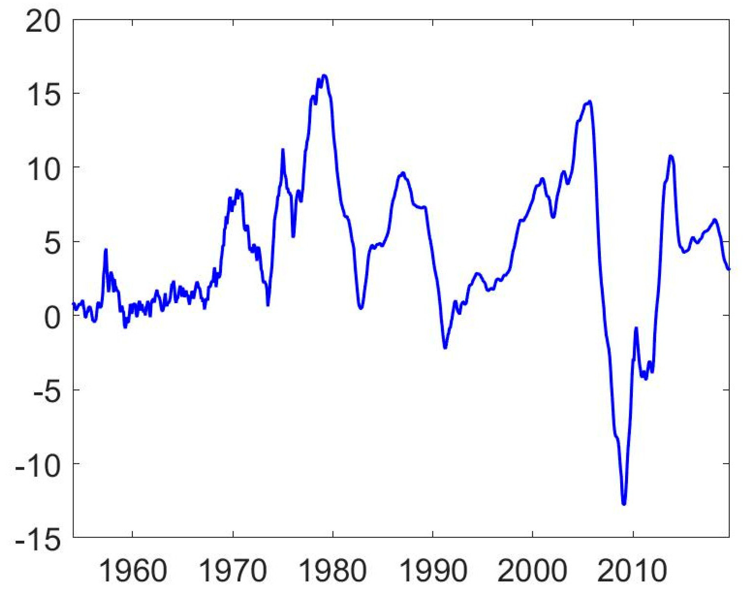
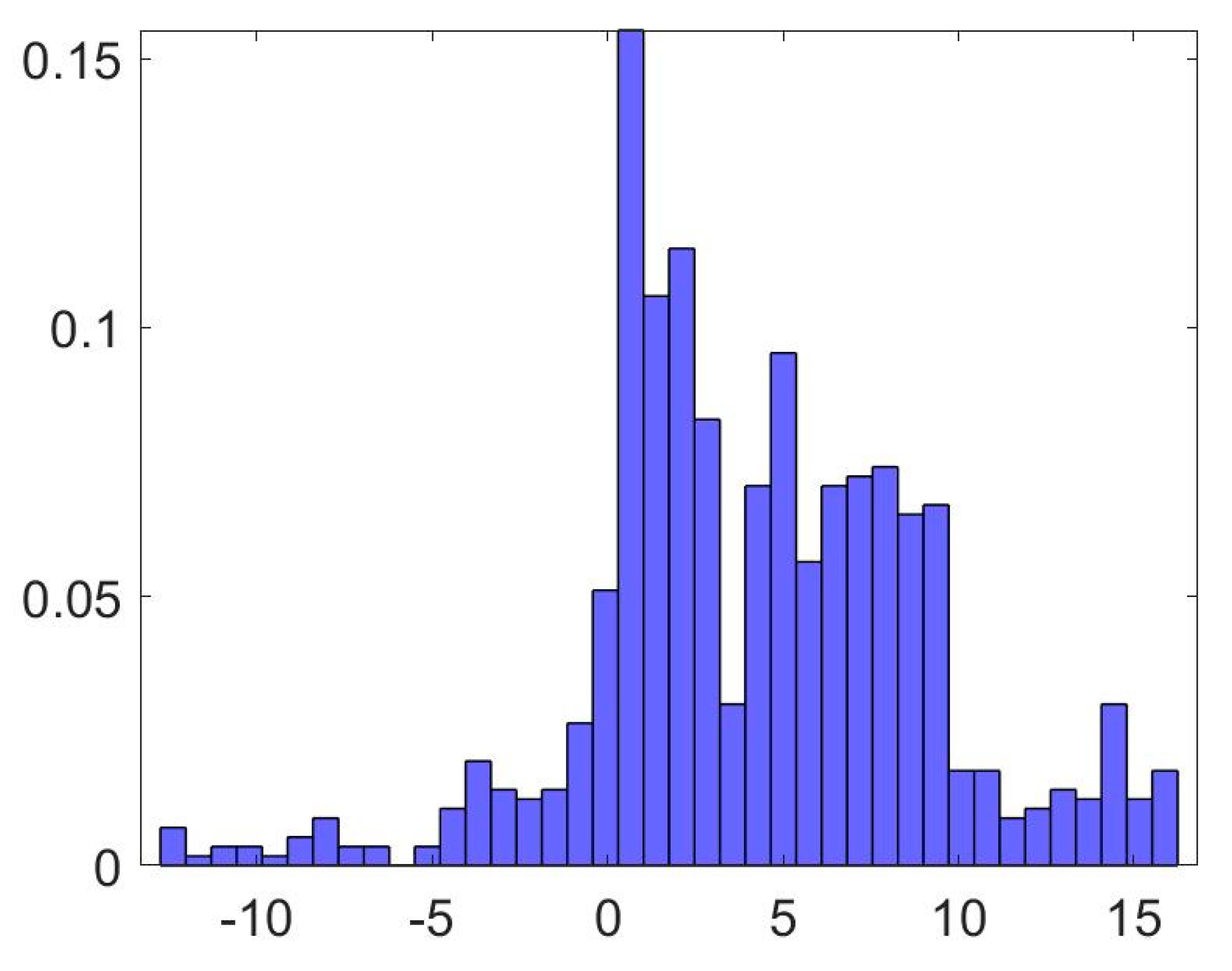
Data are monthly and span the period from January 1953 to September 2019. Nominal returns are calculated as , where is the price index at time t. A time-series plot of the return data is given in Figure 1 and a histogram showing the unconditional distribution is provided in Figure 2. Some key descriptive statistics are given in Table 1.
As both the histogram in Figure 2 and the descriptive statistics in Table 1 suggest, the tails of the distribution appear heavier than what is implied by a normal distribution; the kurtosis of the unconditional distribution is around 3.8. There is also a slight negative skewness. Taken together, this means that the Jarque–Bera test strongly rejects an assumption of normality. Furthermore, both the Augmented Dickey–Fuller test and the KPSS test strongly suggest that the return series does not contain a unit root.
In Table 2, we compare the unconditional housing-price returns and a normally distributed variable using the kurtosis (), peakedness () and tailness () measures proposed by Liu (2019). These measures are based on the ratio of interquantile ranges of the variables, using various quantiles of the distribution denoted by , , and (for example, means that we use the 5th percentile of the distribution when calculating kurtosis and tailness).2 Of particular importance are the tails of the return distribution, which are heavier than those of the normal distribution at all levels. There is also some evidence for asymmetry in the unconditional distribution further out in the tails (α = 0.01), but skewness is not a robust feature if we use different quantiles (α).
4. Methodological Framework
Since the focus of our analysis was to model the properties of the housing-return series, we used univariate time series to capture the dynamics of the returns. We used AR models because they typically perform well in macroeconomic forecasting (e.g., Faust and Wright 2009), despite their simplicity and parsimony. Our baseline model is the homoscedastic univariate AR(p) model:
where is assumed to be an iid normal error term, . The number of lags is determined using the Schwarz (1978) information criterion, which suggests a lag length of = 5; for comparability we employed the same number of lags across all model specifications.
We then allowed for a more flexible error term in the model. First, we let the second moment vary over time. Doing that, we choose a robust approach and rely on the GARCH(1,1) specification (Bollerslev 1986), with a normally distributed error term. This is a common modelling choice—see Chung et al. (2012) and Clark and Ravazzolo (2015) among others for macroeconomic variables—and for financial data, a GARCH(1,1) model is fairly difficult to outperform (Hansen and Lunde 2005). Hence, the second model was the AR(p)-GARCH(1,1):
where , as above, is assumed to be an iid, normal error term. In the third and fourth models, we relax the assumption of normality of the error term, while maintaining symmetry. This is done by using and , where is the degrees of freedom. Of specific interest here is the fact that both the Laplace distribution and the Student-t distribution allow for heavier-than-Gaussian tails.3 Finally, in the fifth model, we assume that the error terms are drawn from the Skew-t distribution (Hansen 1994)—that is, , where is the degrees of freedom and is the skewness parameter. This means that we allowed for both heavy tails and asymmetry in the error term.4
Our primary focus was to evaluate which distributional properties are important for modelling the dynamics of the housing-price return series. We evaluated this based on both within-sample estimates (using maximum likelihood) and an out-of-sample forecasting exercise; in the latter, we considered both point and density forecasts. The point forecasts were evaluated based on the root mean square error (RMSE) of the forecast, accompanied by the Diebold–Mariano test (Diebold and Mariano 1995). We formulated the test such that a positive test value implies that the given model outperforms the benchmark.5
In terms of density forecast evaluation, we made use of the probability integral transform (PIT) proposed by Diebold et al. (1998). We looked at the histograms of the PIT and visually assessed how close they are to the uniform distribution. We also employed more rigorous statistical techniques such as the Kullbach–Leibler (KL) divergence (Kullback and Leibler 1951) of the PIT series from an iid uniform distribution and formal statistical tests of uniformity, namely, the Kolmogorov–Smirnov (KS) and the Anderson–Darling (AD) test (Anderson and Darling 1952).6 For all these measures, a lower value implies that the given model produces a better density forecast.
5. Empirical Analysis
We start by presenting within-sample estimation results for all five specifications.7,8 After that, we turn to an out-of-sample forecast exercise. In the forecast exercise, we focus on the one-period-ahead horizon. The main reason for this is that results for that horizon theoretically are most closely related to within-sample findings and can hence be considered a validation tool.
5.1. Within-Sample Estimation Results
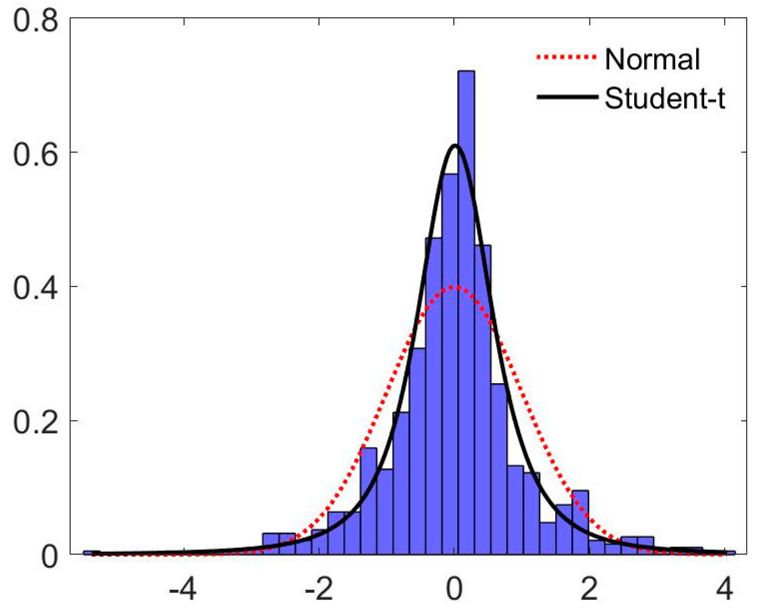
Table 3 presents the estimation results for the five specifications. Note that the housing-price return series is fairly persistent (the sum of the autoregressive coefficients are close to unity). Engle’s (1982) ARCH test shows the strong presence of conditional heteroscedasticity for the residuals in the baseline model in column 1. Also, the Jarque–Bera test suggests that residuals are non-Gaussian in this specification. This is further supported by Figure 3, where it is clear that a t-distribution fits the residuals of the baseline specification better than a normal distribution.
The GARCH(1,1) specification (column 2) seems to take care of conditional heteroscedasticity quite well. However, the variance is very persistent and its parameters are not precisely estimated.9 For the specification with Laplace distribution, where no extra parameter is added to capture heavy-tails, the persistence of the variance is somewhat lower. However, it seems that the Laplace distribution is not flexible enough to capture the behaviour of the standardised residuals, as their transformation by imposing a normal distribution still shows signs of non-Gaussianity according to the Jarque–Bera test.10 In contrast, the more flexible approaches, the t and the Skew-t distribution, seem appropriate to capture non-Gaussianity. However, the skewness parameter is low and non-significant (column 5).
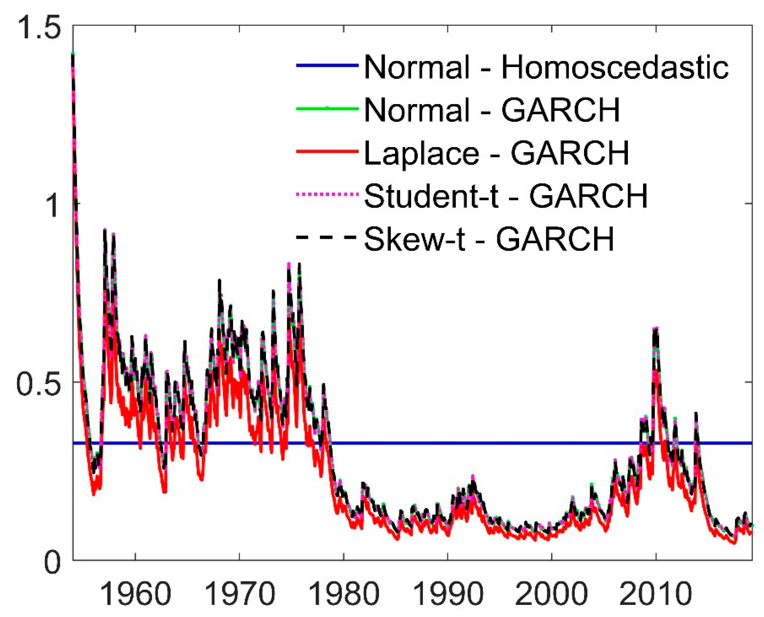
Figure 4 shows the estimated conditional volatility of the return series. All GARCH specifications look quite similar; the biggest discrepancy is found for the Laplace, which due to its excessively heavy tails allows for a generally lower variance. Volatility also clusters; the series starts out with a higher general level of volatility, is considerably lower between 1980 and 2005, and peaks again during the financial crisis.
Having assessed the different specifications within-sample, we next conducted an out-of-sample forecast exercise to validate our results. If we can establish with this exercise that a more complex specification also generates better out-of-sample forecasts, we can conclude that our results are not due to over-fitting the data within-sample.
5.2. Out-of-Sample Analysis
We evaluated the one-period-ahead forecasting performance of the models using an expanding window technique starting in January 1974; this yielded F = 548 forecasts to evaluate.11 The results are collected in Table 4 for both point and density forecast measures.
For point forecasts, the homoscedastic model clearly performs worst. Accounting for time-varying volatility statistically significantly improves the forecast, as can be seen from the Diebold–Mariano test. However, allowing for non-Gaussian error terms does not provide additional improvement in point forecasts over the Gaussian GARCH specification.
For density forecasts, the homoscedastic benchmark model again appears to have the weakest performance. Not only are all three evaluation measures largest for this model, the KS and AD tests reject uniformity of the PIT series at the five percent level. Comparing the results in Table 4, allowing for GARCH effects (coupled with normally distributed error terms) improves quite a lot on the density forecasts such that the formal tests no longer reject the null of uniformity. Additional improvements are generated by allowing for heavier tails in the error distribution using a t-distributed error term. Further generalising the error distribution to a Skew-t distribution appears to be less important, although all three density forecast measures are lowest in case of the specification with skewed error terms. Using the Laplace distribution to capture non-Gaussianity seems to produce the least favourable results (with the KS and AD tests rejecting uniformity), which is consistent with the within-sample findings.
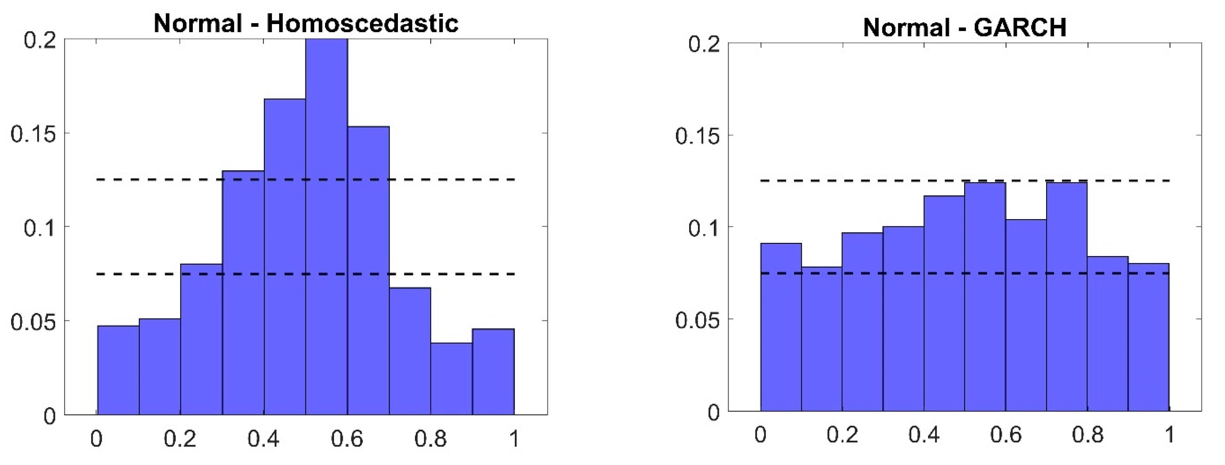
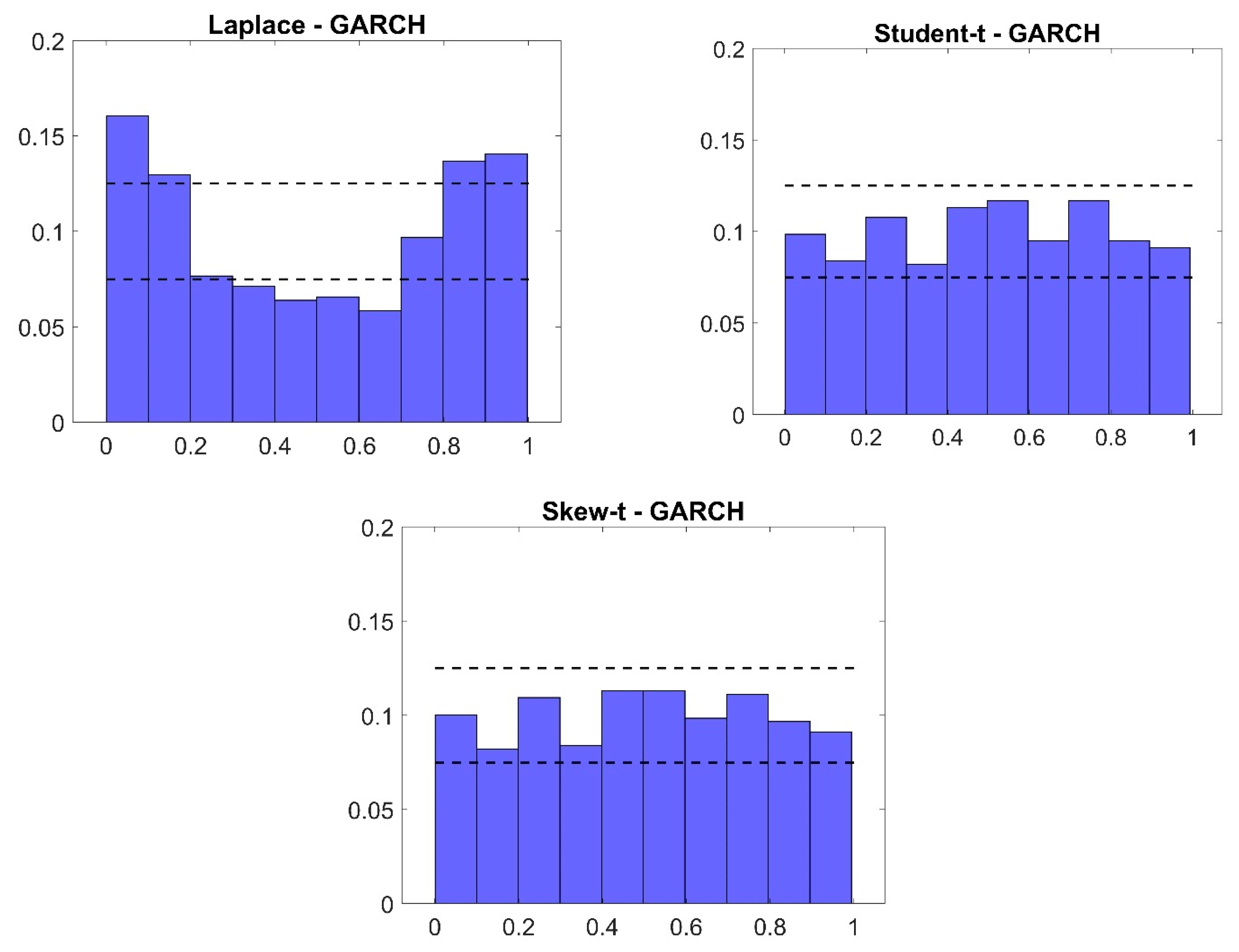
To gain further insight into the out-of-sample results, the histograms of the PIT for each specification are presented in Figure A1 in Appendix A. The graph of the homoscedastic model (top left panel in Figure A1) is peaked, implying that the homoscedastic, Gaussian model’s predictive density is too wide.12 Allowing for GARCH effects—while still assuming a Gaussian error term—eliminates this problem and produces PITs whose distribution is fairly close to uniform (top right panel in Figure A1). The Laplace distribution is less successful at capturing the tail observations (second row, left panel in Figure A1), while the Student-t, and Skew-t distributed error terms appear most successful in bringing PITs close to uniformity (bottom left and right panels in Figure A1, respectively).
5.3. Discussion of the Results
Our aim with the current study was to assess whether non-Gaussianity in housing returns is important when it comes to modelling the dynamics of the series (which is also related to point and density forecasting). Our results clearly point to the conclusion that non-Gaussianity does matter. The in-sample evidence shows that we need to use distributions that are different from the Gaussian to capture the behaviour of the innovations; the model with conditionally heteroscedastic, but Gaussian error terms has standardised innovations that are non-normal, as evidenced by the Jarque–Bera test. Furthermore, we found a need for flexible modelling of the distribution: either a t-distribution or a Skew-t distribution (both of which parametrise the degree of non-Gaussianity) can capture the shape of the innovation distributions appropriately.
Point forecasts are mostly unaffected by flexible modelling of innovations. This is unsurprising since these additional features introduce more parameters (and hence potentially lower precision) without any changes in the structure of the mean equation. In contrast, the best density forecasts are produced by the models with t- or skew-t innovations (although GARCH effects seem to be most relevant for density forecasts). This underlines the importance of non-Gaussianity in situations where the forecaster is interested not only in the first moment, but the entire predictive distribution. A prime example is fan charts used in monetary policy decision making and communication; see, for example, Cogley et al. (2005). Another example is “growth-at-risk”, which is a framework for providing statements concerning the probability of poor outcomes for GDP growth; see, for example, Adrian et al. (2018); Adrian et al. (2019) and Prasad et al. (2019). Growth-at-risk is getting increasing attention from institutions such as the IMF and central banks.
Our results further strengthen the message of the literature (Myer and Webb 1994; Maurer et al. 2004; Young et al. 2006 and Chiang et al. 2012 among others) that non-Gaussianity is a relevant feature of housing returns. These papers, analysing the unconditional distribution of the variables, provide a very important foundation for our analysis, to which we make additions. By modelling the dynamics and allowing for heteroscedasticity, we established whether unconditional non-Gaussianity is caused by conditional heteroscedasticity alone or if innovations are also non-Gaussian. After finding evidence for the latter, we concluded that allowing for time varying second moments is not sufficient; one should also allow for non-Gaussian innovations.13 The importance of non-Gaussian innovations for out-of-sample forecasting is a finding in line with Dufitinema (2021). However, in this paper we go further, as we document the importance of non-Gaussianity for density forecasts as well.
6. Conclusions
Fat tails in housing-price returns have been established in several studies. We contribute to this literature by analysing heavy-tailed behaviour in the context of modelling and forecasting the return series. We found evidence of both conditional heteroscedasticity and non-Gaussian behaviour. Non-Gaussianity mostly takes the form of excess kurtosis, while the support for skewed behaviour is weaker. We also found that accounting for these features helps to improve both point and density forecasts.
Our results highlight the importance of underlying distributional assumptions when modelling housing-price returns. In addition, our findings point to the relevance of considering time-varying volatility when modelling macroeconomic time series; after all, housing-price returns are not only a financial variable but also an important macroeconomic variable. While this aspect of macroeconomic and macro-finance modelling has grown in popularity over the last fifteen years—after having been made popular by Cogley and Sargent (2005) and Primiceri (2005)—we nevertheless believe that it has not been given sufficient attention.
Author Contributions
The authors contributed equally to the manuscript. All authors have read and agreed to the published version of the manuscript.
Funding
The authors gratefully acknowledge financial support from Jan Wallanders och Tom Hedelius stiftelse (grants number Bv18-0018, P18-0201 and W19-0021).
Institutional Review Board Statement
Not applicable.
Informed Consent Statement
Not applicable.
Data Availability Statement
Data are available upon reasonable request from the corresponding author.
Acknowledgments
We are grateful to the editor and two anonymous reviewers for their helpful comments and suggestions.
Conflicts of Interest
There is no conflict of interest to disclose.
Appendix A
Figure A1.
Histograms of probability integral transform for out–of–sample forecasts. Note: Relative frequency on vertical axis.
Figure A1.
Histograms of probability integral transform for out–of–sample forecasts. Note: Relative frequency on vertical axis.


Table A1.
Within–sample estimation results, January 1975 to September 2019.
| (1) | (2) | (3) | (4) | (5) | ||
|---|---|---|---|---|---|---|
| Mean equation [AR(5)] | 0.028 | 0.031 | 0.033 | 0.028 | 0.026 | |
| (0.032) | (0.003) | (0.000) | (0.004) | (0.010) | ||
| 1.909 | 1.970 | 1.937 | 1.970 | 1.970 | ||
| (0.000) | (0.000) | (0.000) | (0.000) | (0.000) | ||
| −0.919 | −0.897 | −0.838 | −0.909 | −0.915 | ||
| (0.000) | (0.000) | (0.000) | (0.000) | (0.000) | ||
| −0.234 | −0.469 | −0.538 | −0.454 | −0.438 | ||
| (0.018) | (0.000) | (0.000) | (0.000) | (0.000) | ||
| 0.430 | 0.640 | 0.717 | 0.638 | 0.627 | ||
| (0.000) | (0.000) | (0.000) | (0.000) | (0.000) | ||
| −0.192 | −0.249 | −0.284 | −0.250 | −0.248 | ||
| (0.000) | (0.000) | (0.000) | (0.000) | (0.000) | ||
| GARCH equation | 0.001 | 0.001 | 0.001 | 0.001 | ||
| (0.003) | (0.010) | (0.008) | (0.006) | |||
| 0.215 | 0.124 | 0.192 | 0.188 | |||
| (0.000) | (0.001) | (0.000) | (0.000) | |||
| 0.742 | 0.724 | 0.759 | 0.762 | |||
| (0.000) | (0.000) | (0.000) | (0.000) | |||
| Degrees of freedom | 6.734 | 6.958 | ||||
| [1.948] | [2.020] | |||||
| Skewness parameter | −0.065 | |||||
| (0.283) | ||||||
| ARCH-test | 115.610 | 8.634 | 8.082 | 8.094 | 8.032 | |
| (0.000) | (0.734) | (0.778) | (0.777) | (0.783) | ||
| JB-test | 1817.200 | 49.303 | 9.748 a | 1.758 a | 0.201 a | |
| (0.000) | (0.000) | (0.008) | (0.415) | (0.904) | ||
| N | 537 | 537 | 537 | 537 | 537 |
Note: Model (1) is a homoscedastic model with Gaussian error terms. Model (2) employs a GARCH(1,1) specification with Gaussian error terms. Models (3), (4) and (5) employ a GARCH(1,1) specification together with Laplace, t–, and Skew–t–distributed error terms, respectively. The ARCH–test is Engle’s test for conditional heteroscedasticity (Engle 1982) conducted with twelve lags. The JB–test is the Jarque–Bera test for conditional heteroscedasticity. “a” indicates that the test is based on the probability integral transform of the (standardised) residuals (see footnote 10). p–values are in parentheses (); standard errors for the degrees of freedom of the t-distribution are in brackets [].“N” is the number of observations.
Appendix B
Table A2.
Descriptive statistics, Jarque–Bera and unit–root test statistic—real returns.
| Mean | Variance | Skewness | Kurtosis | Jarque–Bera | ADF | KPSS | N |
|---|---|---|---|---|---|---|---|
| 0.739 | 18.405 | −0.246 | 3.757 | 26.785 | −3.322 | 0.149 | 789 |
Note: N is the number of observations. The critical value at the five percent level of the Jarque–Bera test is 5.99. The Augmented–Dickey Fuller (ADF) test is performed with four lagged differences in the test equation. Both unit-root tests are performed under the assumption that there is no deterministic trend in the data (the test equation has an intercept but no time trend). The critical value at the five percent level for the ADF and KPSS test is −2.866 and 0.463, respectively.
Table A3.
Comparison of quantile–based kurtosis, peakedness and tailness—real returns.
| Normal distribution | 0.010 | 3.449 | 1.706 | 2.022 | 1.011 | 1.011 |
| 0.025 | 2.906 | 1.706 | 1.704 | 0.852 | 0.852 | |
| 0.050 | 2.439 | 1.706 | 1.430 | 0.715 | 0.715 | |
| Unconditional returns | 0.010 | 4.423 | 1.784 | 2.479 | 1.103 | 1.375 |
| 0.025 | 3.413 | 1.784 | 1.913 | 1.003 | 0.910 | |
| 0.050 | 2.795 | 1.784 | 1.566 | 0.815 | 0.751 |
Note: Comparison of the quantile–based kurtosis, peakedness and tailness among a normal random variable and the unconditional housing–price returns. The measurements are calculated based on ratios of interquantile ranges with α = (0.01, 0.025, 0.05) and η = 0.125, τ = 0.25 quantile levels (see footnote 2 and Liu 2019).
Table A4.
Within–sample estimation results—real returns.
| (1) | (2) | (3) | (4) | (5) | ||
|---|---|---|---|---|---|---|
| Mean equation [AR(5)] | 0.010 | 0.022 | 0.023 | 0.023 | 0.023 | |
| (0.524) | (0.134) | (0.000) | (0.092) | (0.106) | ||
| 1.392 | 1.407 | 1.409 | 1.419 | 1.419 | ||
| (0.000) | (0.000) | (0.000) | (0.000) | (0.000) | ||
| −0.328 | −0.352 | −0.316 | −0.364 | −0.364 | ||
| (0.000) | (0.000) | (0.000) | (0.000) | (0.000) | ||
| −0.078 | −0.069 | −0.097 | −0.070 | −0.069 | ||
| (0.231) | (0.283) | (0.000) | (0.294) | (0.297) | ||
| 0.103 | 0.102 | 0.069 | 0.106 | 0.105 | ||
| (0.100) | (0.098) | (0.001) | (0.094) | (0.085) | ||
| −0.101 | −0.100 | −0.077 | −0.102 | −0.102 | ||
| (0.005) | (0.005) | (0.000) | (0.005) | (0.004) | ||
| GARCH equation | 0.003 | 0.002 | 0.003 | 0.003 | ||
| (0.078) | (0.180) | (0.158) | (0.158) | |||
| 0.087 | 0.077 | 0.105 | 0.105 | |||
| (0.000) | (0.001) | (0.000) | (0.000) | |||
| 0.898 | 0.859 | 0.886 | 0.886 | |||
| (0.000) | (0.000) | (0.000) | (0.000) | |||
| Degrees of freedom | 9.672 | 9.676 | ||||
| [2.882] | [3.810] | |||||
| Skewness parameter | 0.004 | |||||
| (0.080) | ||||||
| ARCH-test | 96.036 | 29.762 | 28.187 | 28.455 | 28.439 | |
| (0.000) | (0.003) | (0.005) | (0.005) | (0.005) | ||
| JB-test | 11.867 | 20.310 | 17.761 a | 0.105 a | 0.067 a | |
| (0.006) | (0.000) | (0.000) | (0.949) | (0.967) | ||
| N | 789 | 789 | 789 | 789 | 789 |
Note: Model (1) is a homoscedastic model with Gaussian error terms. Model (2) employs a GARCH(1,1) specification with Gaussian error terms. Models (3), (4) and (5) employ a GARCH(1,1) specification together with Laplace, t–, and Skew–t–distributed error terms, respectively. The ARCH-test is Engle’s test for conditional heteroscedasticity (Engle 1982) conducted with twelve lags. The JB-test is the Jarque–Bera test for conditional heteroscedasticity. “a” indicates that the test is based on the probability integral transform of the (standardised) residuals (see footnote 10). p–values are in parentheses (); standard errors for the degrees of freedom of the t–distribution are in brackets []. “N” is the number of observations.
Table A5.
Forecast evaluation results—real returns.
| RMSE | DM | KS | AD | KL | |
|---|---|---|---|---|---|
| Normal—Homoscedastic | 0.435 | - | 0.093 | 5.419 | 0.038 |
| Normal—GARCH | 0.432 | 1.864 | 0.065 | 2.501 | 0.021 |
| Laplace—GARCH | 0.434 | 0.183 | 0.112 | 14.240 | 0.068 |
| Student-t—GARCH | 0.431 | 2.003 | 0.058 | 2.152 | 0.015 |
| Skew-t—GARCH | 0.431 | 2.007 | 0.060 | 2.070 | 0.016 |
Note: “RMSE” is the root mean squared error of the point forecasts. “DM” is the Diebold–Mariano test statistic where the model with homoscedastic, normally distributed errors is chosen to be the benchmark. The critical value at the five percent level for the Diebold–Mariano test is 1.65. “KS” is the Kolmogorov–Smirnov test statistic. “AD” is the Anderson-Darling test statistic. “KL” is the Kullback–Leibler divergence of the PIT of the residuals from the uniform distribution on the [0, 1] interval. All three density forecast measures are based on the probability integral transform of the density forecasts produced by each model. The results are based on F = 548 out–of–sample forecasts and an expanding window for parameter estimation. The critical value at the five percent level for the Kolmogorov–Smirnov test is 0.058 and for the Anderson–Darling test it is 2.492.
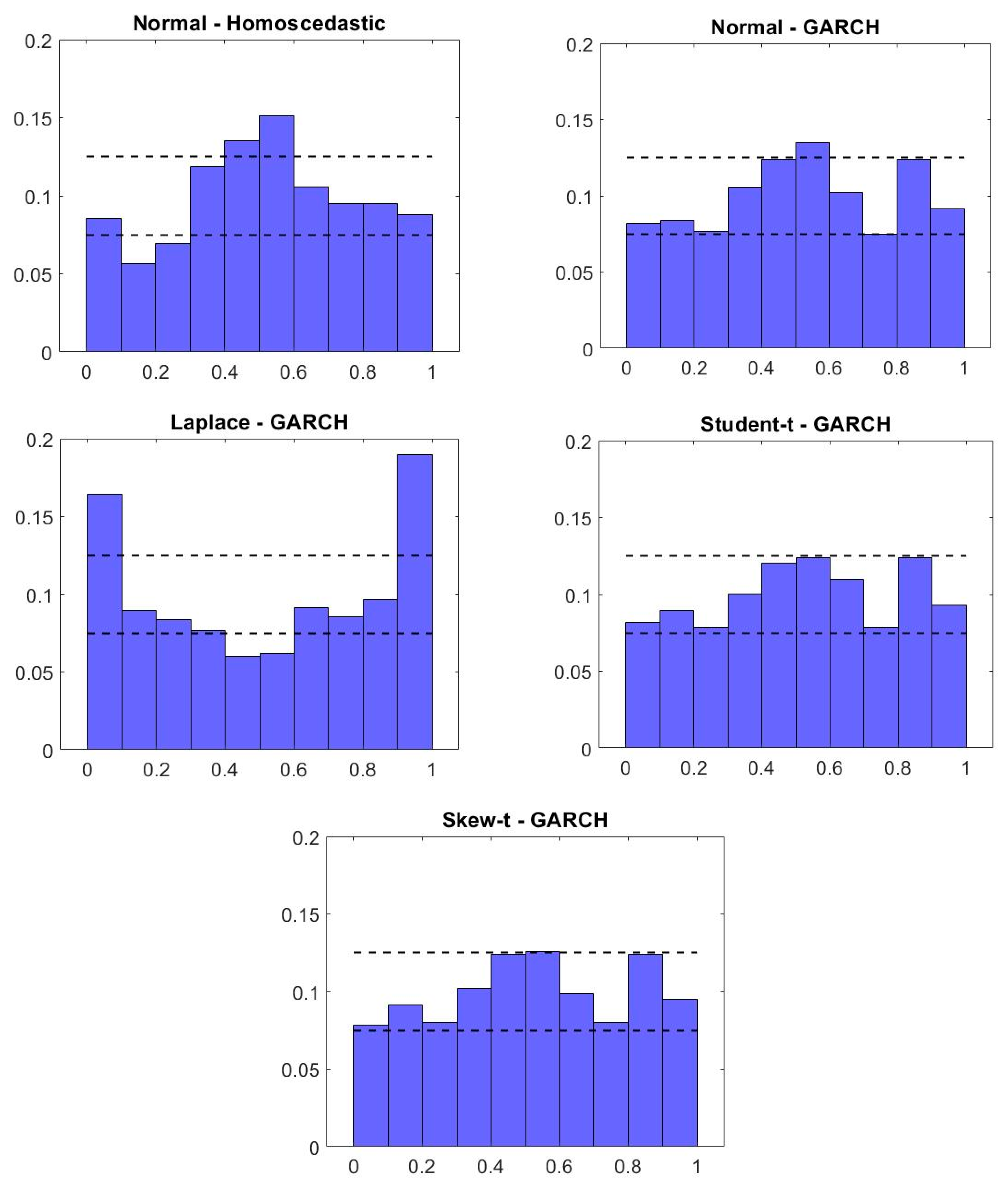
Figure A2.
Histograms of probability integral transform for out–of–sample forecasts—real returns. Note: Relative frequency on vertical axis.
Figure A2.
Histograms of probability integral transform for out–of–sample forecasts—real returns. Note: Relative frequency on vertical axis.

| 1 | The real prices are Shiller’s (2015); the CPI has been used as the deflator. As can be seen when comparing our main results to those in Appendix B, the results using real returns are qualitatively similar. Most importantly, we found that the Student-t GARCH and Skew-t GARCH specifications are the only ones whose residuals pass the Jarque–Bera test for normality. These two models also have the best out-of-sample forecast performance. |
| 2 | The measures are related to each other and the quantiles of the distribution by the formula
|
| 3 | Fagiolo et al. (2008) found the Laplace distribution useful when modelling the fat tails of GDP growth rates. The Student-t distribution has been used more widely in the empirical literature; see, for example, Cúrdia et al. (2014); Clark and Ravazzolo (2015); Cross and Poon (2016); and Kiss and Österholm (2020). |
| 4 | |
| 5 | As pointed out by Diebold (2015), the Diebold and Mariano (1995) test in its standard form is a reasonable choice even if we employ nested models, for which the original assumptions of the test do not formally hold. This is further supported by the fact that the test performs relatively well in such larger training and evaluation samples as the one we use in our analysis (Clark and McCracken 2013). |
| 6 | The KL divergence has been used in a number of applications in the context of density forecasts—typically though with a somewhat different focus; see, for example, Cogley et al. (2005); Robertson et al. (2005); Hall and Mitchell (2007); Diks et al. (2010) and Mitchell and Wallis (2011). |
| 7 | Figure 1 suggests that the time-series behaviour of the return series may have changed around 1975. In fact, the Shiller (2015) dataset changes source in January 1975. Therefore, we also estimate the model on the shorter subsample, namely, January 1975 to September 2019. The results collected in Table A1 in Appendix A are qualitatively very similar to full sample estimates. |
| 8 | We also assessed the robustness of our results to the presence of different regimes, in particular the boom and bust cycle between 2002 and 2009. We did this by allowing for a different constant and dynamics in the mean equation during this period, using a time dummy and interactions. Unreported results (available upon request from the authors) show very similar results to our baseline. Capturing non-Gaussianity in the innovations remains a salient and important feature of the model. |
| 9 | In fact, the parameters and sum up to unity for the normal-GARCH, Student-t-GARCH and Skew-t-GARCH specifications. However, looking at the results using the Laplace distribution and the shorter sample, integrated volatility does not seem to be a robust feature of the data, therefore we do not impose it in any of the specifications with conditional heteroscedasticity. |
| 10 | The Jarque–Bera tests are based on , the PIT series of the standardised residuals, for which is standard normally distributed (where is the inverse cumulative distribution function of the standard normal distribution). We test this by applying the Jarque–Bera test on . |
| 11 | That is, we first estimate the models on the sample January 1953 to January 1974 and make predictions for February 1974. We then expand the sample to January 1953 to February 1974, re-estimate the models and predict March 1974. We continue in this manner until we reach the end of the sample, where we estimate the models using data from January 1953 to August 2019 and make predictions for September 2019. |
| 12 | This finding is concordant with the fact that our within-sample analysis indicates that the unconditional volatility overestimates the conditional one in the larger part of the out-of-sample evaluation period; see Figure 4. |
| 13 | Non-Gaussianity is also important for identifying a housing-price shock in a VAR model. Lanne et al. (2017) show that it is possible to identify an otherwise unidentified structural VAR model by deviating from the Gaussian assumption. That helps solve the problem discussed in Musso et al. (2011), namely, that housing-price shocks are not identified in a VAR model with Gaussian error terms. |
References
- Acemoglu, Daron, and Andrew Scott. 1997. Asymmetric business cycles: Theory and time-series evidence. Journal of Monetary Economics 40: 501–33. [Google Scholar] [CrossRef] [Green Version]
- Acolin, Arthur. 2020. Housing wealth and consumption over the 2001–2013 period: The role of the collateral channel. Journal of Housing Research 29: 68–88. [Google Scholar] [CrossRef]
- Adrian, Tobias, Federico Grinberg, Nellie Liang, and Shehereya Malik. 2018. The Term Structure of Growth-at-Risk. Working Paper 18/180. Washington, DC, USA: International Monetary Fund. [Google Scholar]
- Adrian, Tobias, Nina Boyarchenko, and Domenico Giannone. 2019. Vulnerable growth. American Economic Review 109: 1263–89. [Google Scholar] [CrossRef] [Green Version]
- Ahamada, Ibrahim, and Jose Luis Diaz Sanchez. 2013. A Retrospective Analysis of the House Prices Macro-Relationship in the United States. World Bank Policy Research Working Paper 6549. Available online: https://ssrn.com/abstract=2303105 (accessed on 15 July 2021).
- Anderson, Theodore W., and Donald A. Darling. 1952. Asymptotic theory of certain goodness of fit criteria based on stochastic processes. Annals of Mathematical Statistics 23: 193–212. [Google Scholar] [CrossRef]
- Ascari, Guido, Giorgio Fagiolo, and Andrea Roventini. 2015. Fat-tail distributions and business-cycle models. Macroeconomic Dynamics 19: 465–76. [Google Scholar] [CrossRef] [Green Version]
- Bekaert, Geert, and Alexander Popov. 2019. On the link between the volatility and skewness of growth. IMF Economic Review 67: 746–90. [Google Scholar] [CrossRef] [Green Version]
- Bollerslev, Tim. 1986. Generalized autoregressive conditional heteroskedasticity. Journal of Econometrics 31: 307–27. [Google Scholar] [CrossRef] [Green Version]
- Campbell, John Y., and Joao F. Cocco. 2007. How do house prices affect consumption? Evidence from micro data. Journal of Monetary Economics 54: 591–621. [Google Scholar] [CrossRef] [Green Version]
- Case, Karl E., and Robert J. Shiller. 1989. The efficiency of the market for single-family homes. The American Economic Review 79: 125–37. [Google Scholar]
- Catte, Pietro, Nathalie Girouard, Robert Price, and Christophe André. 2004. Housing Markets, Wealth and the Business Cycle. OECD Economics Working Paper 394. Available online: https://0-doi-org.brum.beds.ac.uk/10.1787/534328100627 (accessed on 15 May 2021).
- Chiang, Ming-Chu, I-Chun Tsai, and Cheng-Feng Lee. 2012. The Downside Risk of US and UK Housing Markets. Journal of Real Estate Portfolio Management 18: 257–72. [Google Scholar] [CrossRef]
- Chung, Hess, Jean-Philippe Laforte, David Reifschneider, and John C. Williams. 2012. Have we underestimated the likelihood and severity of zero lower bound events? Journal of Money, Credit and Banking 44: 47–82. [Google Scholar] [CrossRef]
- Clark, Todd E., and Michael McCracken. 2013. Advances in forecast evaluation. In Handbook of Economic Forecasting. Edited by Graham Elliott and Allan Timmermann. Amsterdam: Elsevier, vol. 2, pp. 1107–201. [Google Scholar]
- Clark, Todd E., and Francesco Ravazzolo. 2015. Macroeconomic forecasting performance under alternative specifications of time-varying volatility. Journal of Applied Econometrics 30: 551–75. [Google Scholar] [CrossRef]
- Cogley, Timothy, and Thomas J. Sargent. 2005. Drifts and volatilities: Monetary policies and outcomes in the post WWII US. Review of Economic Dynamics 8: 262–302. [Google Scholar] [CrossRef] [Green Version]
- Cogley, Timothy, Sergei Morozov, and Thomas J. Sargent. 2005. Bayesian fan charts for UK inflation: Forecasting and sources of uncertainty in an evolving monetary system. Journal of Economic Dynamics and Control 29: 1893–925. [Google Scholar] [CrossRef] [Green Version]
- Cross, Jamie, and Aubrey Poon. 2016. Forecasting structural change and fat-tailed events in Australian macroeconomic variables. Economic Modelling 58: 34–51. [Google Scholar] [CrossRef]
- Cúrdia, Vasco, Marco Del Negro, and Daniel L. Greenwald. 2014. Rare shocks, great recessions. Journal of Applied Econometrics 29: 1031–52. [Google Scholar] [CrossRef] [Green Version]
- Diebold, Francis X. 2015. Comparing predictive accuracy, twenty years later: A personal perspective on the use and abuse of Diebold-Mariano tests. Journal of Business and Economic Statistics 33: 1–9. [Google Scholar] [CrossRef] [Green Version]
- Diebold, Francis X., and Robert S. Mariano. 1995. Comparing predictive accuracy. Journal of Business and Economic Statistics 13: 134–44. [Google Scholar]
- Diebold, Francis X., Todd A. Gunther, and Anthony S. Tay. 1998. Evaluating density forecasts with applications to financial risk management. International Economic Review 39: 863–83. [Google Scholar] [CrossRef] [Green Version]
- Diks, Cees, Valentyn Panchenko, and Dick Van Dijk. 2010. Out-of-sample comparison of copula specifications in multivariate density forecasts. Journal of Economic Dynamics and Control 34: 1596–609. [Google Scholar] [CrossRef] [Green Version]
- Dufitinema, Josephine. 2021. Stochastic volatility forecasting of the Finnish housing market. Applied Economics 53: 98–114. [Google Scholar] [CrossRef]
- Engle, Robert F. 1982. Autoregressive conditional heteroscedasticity with estimates of the variance of United Kingdom inflation. Econometrica 50: 987–1007. [Google Scholar] [CrossRef]
- Fagiolo, Giorgio, Mauro Napoletano, and Andrea Roventini. 2008. Are output growth-rate distributions fat-tailed? Some evidence from OECD countries. Journal of Applied Econometrics 23: 639–69. [Google Scholar] [CrossRef] [Green Version]
- Faust, Jon, and Jonathan H. Wright. 2009. Comparing Greenbook and reduced form forecasts using a large realtime dataset. Journal of Business and Economic Statistics 27: 468–79. [Google Scholar] [CrossRef] [Green Version]
- Foster, Chester, and Robert Van Order. 1984. An option-based model of mortgage default. Housing Finance Review 3: 351. [Google Scholar]
- Graff, Richard, Adrian Harrington, and Michael Young. 1997. The shape of Australian real estate return distributions and comparisons to the United States. Journal of Real Estate Research 14: 291–308. [Google Scholar] [CrossRef]
- Granziera, Eleonora, and Sharon Kozicki. 2015. House price dynamics: Fundamentals and expectations. Journal of Economic Dynamics and Control 60: 152–65. [Google Scholar] [CrossRef] [Green Version]
- Hall, Stephen G., and James Mitchell. 2007. Combining density forecasts. International Journal of Forecasting 23: 1–13. [Google Scholar] [CrossRef]
- Hansen, Bruce E. 1994. Autoregressive conditional density estimation. International Economic Review 35: 705–30. [Google Scholar] [CrossRef]
- Hansen, Peter R., and Asger Lunde. 2005. A forecast comparison of volatility models: Does anything beat a GARCH (1, 1)? Journal of Applied Econometrics 20: 873–89. [Google Scholar] [CrossRef] [Green Version]
- Hjalmarsson, Erik, and Pär Österholm. 2020. Heterogeneity in households’ expectations of housing prices-evidence from micro data. Journal of Housing Economics 50: 101731. [Google Scholar] [CrossRef]
- Iacoviello, Matteo. 2005. House prices, borrowing constraints, and monetary policy in the business cycle. American Economic Review 95: 739–64. [Google Scholar] [CrossRef] [Green Version]
- Iacoviello, Matteo, and Stefano Neri. 2010. Housing market spillovers: Evidence from an estimated DSGE model. American Economic Journal: Macroeconomics 2: 125–64. [Google Scholar] [CrossRef] [Green Version]
- Jordá, Óscar, Katharina Knoll, Dmitry Kuvshinov, Mority Schularick, and Alan M. Taylor. 2019. The rate of return on everything, 1870–2015. Quarterly Journal of Economics 134: 1225–98. [Google Scholar] [CrossRef]
- Kiss, Tamás, and Pär Österholm. 2020. Fat tails in leading indicators. Economics Letters 193: 109317. [Google Scholar] [CrossRef]
- Klarl, Torben. 2016. The nexus between housing and GDP re-visited: A wavelet coherence view on housing and GDP for the US. Economics Bulletin 36: 704–20. [Google Scholar]
- Kullback, Solomon, and Richard A. Leibler. 1951. On information and sufficiency. Annals of Mathematical Statistics 22: 79–86. [Google Scholar] [CrossRef]
- Lanne, Markku, Mika Meitz, and Pentti Saikkonen. 2017. Identification and estimation of non-Gaussian structural vector autoregressions. Journal of Econometrics 196: 288–304. [Google Scholar] [CrossRef] [Green Version]
- Leung, Charles Ka Yui, Youngman Chun Fai Leong, and Siu Kei Wong. 2006. Housing price dispersion: An empirical investigation. Journal of Real Estate Finance and Economics 32: 357–85. [Google Scholar] [CrossRef]
- Liu, Xiaochun. 2019. On tail fatness of macroeconomic dynamics. Journal of Macroeconomics 62: 103154. [Google Scholar] [CrossRef]
- Ma, Chao. 2020. Momentum and reversion to fundamentals: Are they captured by subjective expectations of house prices? Journal of Housing Economics 49: 101687. [Google Scholar] [CrossRef]
- Martín-Legendre, Juan, Pablo Castellanos-García, and José Manuel Sánchez-Santos. 2019. Housing and financial wealth effects on consumption: Evidence from the Spanish Survey of Household Finances. Economics Bulletin 39: 1930–40. [Google Scholar]
- Maurer, Raimond, Frank Reiner, and Steffen P. Sebastian. 2004. Financial characteristics of international real estate returns: Evidence from the UK, US, and Germany. Journal of Real Estate Portfolio Management 10: 59–76. [Google Scholar]
- McMillan, David G. 2012. Long-run stock price-house price relation: Evidence from an ESTR model. Economics Bulletin 32: 1737–46. [Google Scholar] [CrossRef] [Green Version]
- Mitchell, James, and Kenneth F. Wallis. 2011. Evaluating density forecasts: Forecast combinations, model mixtures, calibration and sharpness. Journal of Applied Econometrics 26: 1023–40. [Google Scholar] [CrossRef] [Green Version]
- Musso, Alberto, Stefano Neri, and Livio Stracca. 2011. Housing, consumption and monetary policy: How different are the US and the euro area? Journal of Banking and Finance 35: 3019–41. [Google Scholar] [CrossRef] [Green Version]
- Myer, F. C. Neil, and James R. Webb. 1994. Statistical properties of returns: Financial assets versus commercial real estate. Journal of Real Estate Finance and Economics 8: 267–82. [Google Scholar] [CrossRef]
- Neftci, Salih N. 1984. Are economic time series asymmetric over the business cycle? Journal of Political Economy 92: 307–28. [Google Scholar] [CrossRef]
- Pan, Xuefeng, and Weixing Wu. 2021. Housing returns, precautionary savings and consumption: Micro evidence from China. Journal of Empirical Finance 60: 39–55. [Google Scholar] [CrossRef]
- Piazzesi, Monika, and Martin Schneider. 2009. Momentum traders in the housing market: Survey evidence and a search model. American Economic Review 99: 406–11. [Google Scholar] [CrossRef] [Green Version]
- Pontines, Victor. 2010. Fat-tails and house prices in OECD countries. Applied Economics Letters 17: 1373–77. [Google Scholar] [CrossRef]
- Prasad, Ananthakrishnan, Selim Elekdag, Phakawa Jeasakul, Romain Lafarguette, Adrian Alter, Alan Xiaochen Feng, and Changchun Wang. 2019. Growth at Risk: Concept and Application in IMF Country Surveillance. Working Paper 19/36. Washington, DC, USA: International Monetary Fund. [Google Scholar]
- Primiceri, Giorgio E. 2005. Time varying structural vector autoregressions and monetary policy. Review of Economic Studies 72: 821–52. [Google Scholar] [CrossRef]
- Robertson, John C., Ellis W. Tallman, and Charles H. Whiteman. 2005. Forecasting using relative entropy. Journal of Money, Credit and Banking 37: 383–401. [Google Scholar] [CrossRef] [Green Version]
- Schwarz, Gideon. 1978. Estimating the dimension of a model. Annals of Statistics 6: 461–64. [Google Scholar] [CrossRef]
- Shiller, Robert J. 2015. Irrational Exuberance: Revised and Expanded, 3rd ed. Princeton: Princeton University Press. [Google Scholar]
- Young, Michael S., and Richard A. Graff. 1995. Real estate is not normal: A fresh look at real estate return distributions. Journal of Real Estate Finance and Economics 10: 225–59. [Google Scholar] [CrossRef]
- Young, Michael S., Stephen L. Lee, and Steven P. Devaney. 2006. Non-normal real estate return distributions by property type in the UK. Journal of Property Research 23: 109–33. [Google Scholar] [CrossRef]
Figure 1.
Housing–price return data. Note: Twelve–month change in percent on vertical axis.

Figure 2.
Histogram of housing–price return data. Note: Twelve–month change in percent on horizontal. Relative frequency on vertical axis.
Figure 2.
Histogram of housing–price return data. Note: Twelve–month change in percent on horizontal. Relative frequency on vertical axis.

Figure 3.
Residuals from homoscedastic model. Note: Density on vertical axis.

Figure 4.
Conditional volatility under different assumptions for the error term. Note: Conditional standard deviation on vertical axis.
Figure 4.
Conditional volatility under different assumptions for the error term. Note: Conditional standard deviation on vertical axis.

Table 1.
Descriptive statistics of the returns, Jarque–Bera and unit root test statistic.
| Mean | Variance | Skewness | Kurtosis | Jarque–Bera | ADF | KPSS | N |
|---|---|---|---|---|---|---|---|
| 4.278 | 24.390 | −0.150 | 3.813 | 24.464 | −3.505 | 0.166 | 789 |
Note: N is the number of observations. The critical value at the five percent level of the Jarque–Bera test is 5.99. The Augmented Dickey–Fuller (ADF) test is performed with four lagged differences in the test equation (to be consistent with the selected lag length for the empirical model considered in Section 5). Both unit-root tests are performed under the assumption that there is no deterministic trend in the data (the test equation has an intercept but no time trend). The critical value at the five percent level for the ADF and KPSS test is −2.866 and 0.463, respectively.
Table 2.
Comparison of quantile–based kurtosis, peakedness and tailness.
| Normal distribution | 0.010 | 3.449 | 1.706 | 2.022 | 1.011 | 1.011 |
| 0.025 | 2.906 | 1.706 | 1.704 | 0.852 | 0.852 | |
| 0.050 | 2.439 | 1.706 | 1.430 | 0.715 | 0.715 | |
| Unconditional returns | 0.010 | 3.979 | 1.404 | 2.834 | 1.256 | 1.579 |
| 0.025 | 3.317 | 1.404 | 2.363 | 1.141 | 1.222 | |
| 0.050 | 2.615 | 1.404 | 1.862 | 1.013 | 0.850 |
Note: Comparison of the quantile–based kurtosis, peakedness and tailness among a normal random variable and the unconditional housing–price returns. The measurements are calculated based on ratios of interquantile ranges with α = (0.01, 0.025, 0.05) and η = 0.125, τ = 0.25 quantile levels (see Footnote 2 and Liu 2019).
Table 3.
Within–sample estimation results.
| (1) | (2) | (3) | (4) | (5) | ||
|---|---|---|---|---|---|---|
| Mean equation [AR(5)] | 0.038 | 0.033 | 0.035 | 0.033 | 0.032 | |
| (0.023) | (0.185) | (0.000) | (0.467) | (0.013) | ||
| 1.564 | 1.816 | 1.823 | 1.820 | 1.819 | ||
| (0.000) | (0.000) | (0.000) | (0.000) | (0.000) | ||
| −0.509 | −0.756 | −0.743 | −0.741 | −0.740 | ||
| (0.000) | (0.000) | (0.000) | (0.023) | (0.000) | ||
| −0.115 | −0.271 | −0.321 | −0.307 | −0.303 | ||
| (0.103) | (0.011) | (0.000) | (0.147) | (0.020) | ||
| 0.203 | 0.396 | 0.415 | 0.400 | 0.397 | ||
| (0.003) | (0.209) | (0.000) | (0.000) | (0.006) | ||
| −0.152 | −0.189 | −0.180 | −0.178 | −0.178 | ||
| (0.000) | (0.263) | (0.000) | (0.001) | (0.003) | ||
| GARCH equation | 0.000 | 0.000 | 0.001 | 0.001 | ||
| (0.745) | (0.260) | (0.895) | (0.702) | |||
| 0.172 | 0.123 | 0.175 | 0.175 | |||
| (0.459) | (0.001) | (0.824) | (0.671) | |||
| 0.828 | 0.804 | 0.825 | 0.825 | |||
| (0.000) | (0.000) | (0.000) | (0.001) | |||
| Degrees of freedom | 7.870 | 7.941 | ||||
| [26.854] | [3.297] | |||||
| Skewness parameter | −0.031 | |||||
| (0.854) | ||||||
| ARCH-test | 131.592 | 13.661 | 14.431 | 13.440 | 13.494 | |
| (0.000) | (0.322) | (0.274) | (0.338) | (0.334) | ||
| JB-test | 295.989 | 51.528 | 15.288 a | 0.616 a | 0.070 a | |
| (0.000) | (0.000) | (0.000) | (0.735) | (0.966) | ||
| N | 789 | 789 | 789 | 789 | 789 |
Note: Model (1) is a homoscedastic model with Gaussian error terms. Model (2) employs a GARCH(1,1) specification with Gaussian error terms. Models (3), (4) and (5) employ a GARCH(1,1) specification together with Laplace, t–, and Skew–t–distributed error terms, respectively. The ARCH-test is Engle’s test for conditional heteroscedasticity (Engle 1982) conducted with twelve lags. The JB–test is the Jarque–Bera test for conditional heteroscedasticity. “a” indicates that the test is based on the probability integral transform of the (standardised) residuals (see footnote 10). p–values are in parentheses (); standard errors for the degrees of freedom of the t-distribution are in brackets []. “N” is the number of observations.
Table 4.
Forecast evaluation results.
| RMSE | DM | KS | AD | KL | |
|---|---|---|---|---|---|
| Normal—Homoscedastic | 0.279 | - | 0.151 | 25.498 | 0.179 |
| Normal—GARCH | 0.259 | 3.491 | 0.044 | 1.743 | 0.013 |
| Laplace—GARCH | 0.258 | 3.394 | 0.101 | 13.141 | 0.066 |
| Student-t—GARCH | 0.258 | 3.495 | 0.036 | 0.590 | 0.008 |
| Skew-t—GARCH | 0.258 | 3.468 | 0.035 | 0.521 | 0.006 |
Note: “RMSE” is the root mean squared error of the point forecasts. “DM” is the Diebold–Mariano test statistic where the model with homoscedastic, normally distributed errors is chosen to be the benchmark. The critical value at the five percent level for the Diebold–Mariano test is 1.65. “KS” is the Kolmogorov–Smirnov test statistic. “AD” is the Anderson–Darling test statistic. “KL” is the Kullback–Leibler divergence of the PIT of the residuals from the uniform distribution on the [0, 1] interval. All three density forecast measures are based on the PIT of the density forecasts produced by each model. The results are based on F = 548 out-of-sample forecasts and an expanding window for parameter estimation. The critical value at the five percent level for the Kolmogorov–Smirnov test is 0.058 and for the Anderson–Darling test it is 2.492.
Publisher’s Note: MDPI stays neutral with regard to jurisdictional claims in published maps and institutional affiliations. |
© 2021 by the authors. Licensee MDPI, Basel, Switzerland. This article is an open access article distributed under the terms and conditions of the Creative Commons Attribution (CC BY) license (https://creativecommons.org/licenses/by/4.0/).
Share and Cite
MDPI and ACS Style
Kiss, T.; Nguyen, H.; Österholm, P. Modelling Returns in US Housing Prices—You’re the One for Me, Fat Tails. J. Risk Financial Manag. 2021, 14, 506. https://0-doi-org.brum.beds.ac.uk/10.3390/jrfm14110506
AMA Style
Kiss T, Nguyen H, Österholm P. Modelling Returns in US Housing Prices—You’re the One for Me, Fat Tails. Journal of Risk and Financial Management. 2021; 14(11):506. https://0-doi-org.brum.beds.ac.uk/10.3390/jrfm14110506
Chicago/Turabian StyleKiss, Tamás, Hoang Nguyen, and Pär Österholm. 2021. "Modelling Returns in US Housing Prices—You’re the One for Me, Fat Tails" Journal of Risk and Financial Management 14, no. 11: 506. https://0-doi-org.brum.beds.ac.uk/10.3390/jrfm14110506