
Skewed Binary Regression to Study Rental Cars by Tourists in the Canary Islands

 , , and
Abstract
:1. Introduction
2. Methodology
2.1. Logistic Specification
2.2. Bayesian Symmetric Specification
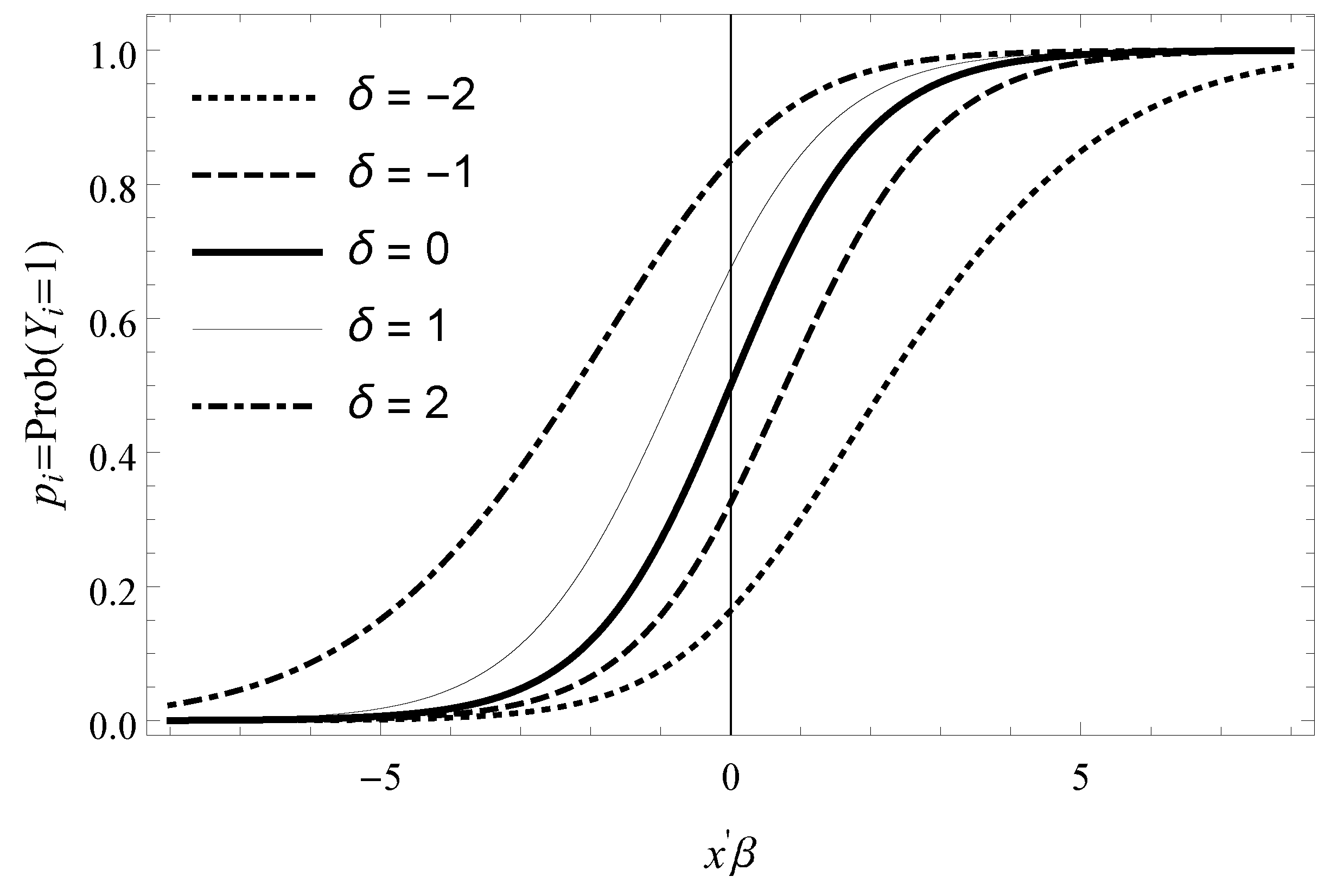
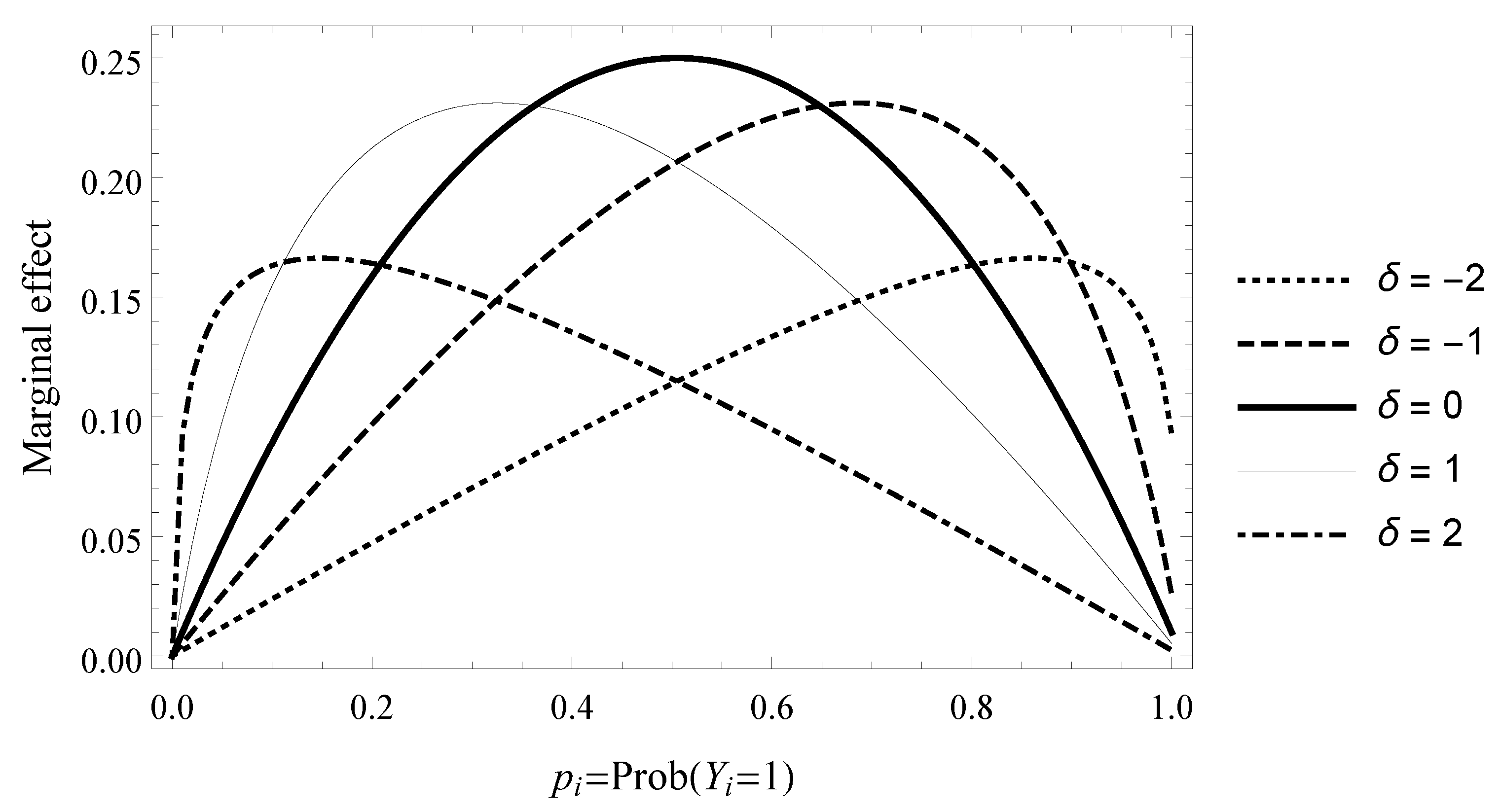
2.3. Bayesian Asymmetric Specification
3. Description of Database
- Origin spent. A quantitative variable defining expenses at origin per person and day. Expenditure of tourists is approximately 99.92 euros on average.
- Destination spent. A quantitative variable defining expenses at destination per person and day. Expenditure of tourists is approximately 40.68 euros on average.
- Nights. A quantitative variable representing the length of stay. It results in approximately nine days on average, with a minimum stay of one day and a maximum of 180.
- Previous visits. A dummy variable takes one whether the tourist has visited the Canary Islands before the current trip and 0 otherwise. Approximately 77% of visitors repeat visits.
- Accommodation. A dummy variable takes one if the tourist has been accommodated at a hotel and 0 otherwise.
- Party. A dummy variable takes 1 if the tourist has travelled with someone else and 0 otherwise.
- Booking. A dummy variable takes one if the tourist has booked the holidays at home and 0 otherwise.
- Low cost. A dummy variable, which takes one if the tourist has travelled in a low-cost carrier.
- Season. A categorical variable expressing the time of the year the tourist traveled: January–May, dummy variable which represents traveling from January to May; June–September, a dummy variable for traveling from June to September; and October–December, the reference dummy variable representing trips from October to December.
- 10.
- SunBeach. A dummy variable takes one whether the main reason for visiting the Islands is enjoying sun and beach, and 0, otherwise.
- 11.
- Holiday. A dummy variable takes 1 when the reason for traveling is holidays, and 0 otherwise.
- 12.
- Age in years. It can be seen in Table 1 that, on average, tourists are in their forties. The minimum age of those interviewed is 16 years old, and 9 are the oldest ones.
- 13.
- Gender. A dummy variable takes 1 for males. 49.5% of visitors are men.
- 14.
- Income. An ordered categorical variable which takes the following values: (1): from 12,000 to 24,000 euros; (2): from 24,001 to 36,000 euros; (3): from 36,001 to 48,000 euros; (4): from 48,001 to 60,000 euros; (5): from 60,001 to 72,000 euros; (6): from 72,001 to 84,000 euros; and (7): greater than 84,000 euros. The data reflect on Table 1 that on average, tourist’s income is between 36,000 euros and 48,000 euros.
- 15.
- Job. A dummy variable takes one if the tourist is employed and 0, otherwise. Approximately 82% of visitors are employed.
- 16.
- Nationality. Tourists are separated according to the following countries of residence: Germany, The United Kingdom, Spain, Nordic countries, and others. Mostly, incoming tourists are from the United Kingdom, followed by other countries, Spain, Germany, and Nordic countries. The dummy reference variable is ’Other’.
4. Empirical Results and Discussion
4.1. Brief Explanation of the Computations
4.2. Interpretation of the Results
4.3. Checking the Models
5. Conclusions
Author Contributions
Funding
Institutional Review Board Statement
Informed Consent Statement
Data Availability Statement
Acknowledgments
Conflicts of Interest
References
- Aguiló, Eugeni, Jaume Rosselló, and Mar Vila. 2017. Length of stay and daily tourist expenditure: A joint analysis. Tourism Management Perspectives 21: 10–17. [Google Scholar] [CrossRef]
- Albert, Jim, and Siddhartha Chib. 1995. Bayesian residual analysis for binary response regression models. Biometrika 82: 747–69. [Google Scholar] [CrossRef]
- Alegre, Joaquín, and Llorenç Pou. 2006. The length of stay in the demand for tourism. Tourism Management 27: 1343–55. [Google Scholar] [CrossRef]
- Alkhalaf, Arwa, and Bruno D. Zumbo. 2017. The impact of predictor variable(s) with skewed cell probabilities on Wald tests in binary logistic regression. Journal of Modern Applied Statistical Methods 16: 40–80. [Google Scholar] [CrossRef]
- Akaike, Hirotugu. 1974. A new look at the statistical model identification. IEEE Transactions on Automatic Control 19: 716–23. [Google Scholar] [CrossRef]
- Bazán, Jorge L., Márcia D. Branco, and Heleno Bolfarine. 2006. A Skew Item Response Model. Bayesian Analysis 4: 861–92. [Google Scholar] [CrossRef]
- Bermúdez, Lluis, José María Pérez-Sánchez, Mercedes Ayuso, Emilio Gómez-Déniz, and Francisco José Vázquez-Polo. 2008. A bayesian dichotomous model with asymmetric link for fraud in insurance. Insurance, Mathematics and Economics 42: 779–86. [Google Scholar] [CrossRef]
- Carlin, Bradley, and Nicholas Polson. 1992. Monte Carlo Bayesian methods for discrete regression models and categorical time series. Bayesian Statistics 13: 577–86. [Google Scholar]
- Caron, Renault, Debajyoti Sinha, Dipak K. Dey, and Adriano Polpo. 2018. Categorical data analysis using a skewed Weibull regression model. Entropy 20: 176. [Google Scholar] [CrossRef] [Green Version]
- Chadee, Doren, and Jan Mattson. 1996. An empirical assessment of customer satisfaction in tourism. The Service Industries Journal 16: 305–20. [Google Scholar] [CrossRef]
- Chen, Ming-Hui, Dipak K. Dey, and Qi-Man Shao. 1999. A new skewed link model for dichotomous quantal response data. Journal of the American Statistical Association 94: 1172–86. [Google Scholar] [CrossRef]
- Currier, Christine, and Peter Falconer. 2014. Maintaining sustainable island destinations in Scotland: The role of the transport-tourism relationship. Journal of Destination Marketing & Management 3: 162–72. [Google Scholar]
- Dimatulac, Terence, Hanna Maoh, Shakil Khan, and Mark Ferguson. 2018. Modeling the demand for electric mobility in the Canadian rental vehicle market. Transportation Research Part D 65: 138–50. [Google Scholar] [CrossRef]
- Ekiz, Erdogan, Pradeep Kumar Nair, and Kashif Hussain. 2010. Measuring The Service Quality in Car Rental Services: Purifying RENTQUAL Instrument with Asian Tourists. Paper presented at the 4th Tourism Outlook & 3rd ITSA Conference, Kuala Lumpur, Malaysia, 30 November–3 December. [Google Scholar]
- Ferrer-Rossell, Berta, and Germa Coenders. 2017. Airline type and tourist expenditure: Are full service and low cost carriers converging or diverging? Journal of Air Transport Management 63: 119–25. [Google Scholar] [CrossRef]
- Gilks, Walter R., Sylvia Richardson, and David J. Spiegelhalter. 1995. Introducing Markov Chain Monte Carlo. In Markov Chain Monte Carlo in Practice. Edited by W. R. Gilks, S. Richardson and D. J. Spiegelhalter. London: Chapman and Hall. [Google Scholar]
- Gomes de Menezes, Antonio, and Ainura Uzagalieva. 2012. The Demand of Car Rentals: A Microeconometric Approach with Count Models and Survey Data. Centro de Estudos de Economia Aplicada do Atlántico, CEEApla Working Paper 12: 1–24. [Google Scholar]
- Gómez-Déniz, Emilio, and Jorge Vicente Pérez-Rodríguez. 2019. Modelling distribution of aggregate expenditure on tourism. Economic Modelling 78: 293–308. [Google Scholar] [CrossRef]
- Gómez-Déniz, Emilio, José Boza-Chirino, and Nancy Dávila-Cárdenes. 2020. Tourist tax to promote rentals of low-emission vehicles. Tourism Economics 6: 1354816620946508. [Google Scholar] [CrossRef]
- Koop, Gary. 2003. Bayesian Econometrics. Hoboken: John Wiley & Sons, Inc. [Google Scholar]
- Lemonte, Artur J., and Jorge L. Bazán. 2018. New links for binary regression: An application to coca cultivation in Peru. Test 27: 597–617. [Google Scholar] [CrossRef]
- Lohmann, Guy, and David Duval. 2011. Critical Aspects of the Tourism-Transport Relationship. Contemporary Tourism Reviews. Edited by C. Cooper. Oxford: Goodfellow Publishers. [Google Scholar]
- Lunn, David J., Andrew Thomas, Nicky Best, and David Spiegelhalter. 2000. Winbugs: A Bayesian modelling framework: Concepts, structure, and extensibility. Statistics and Computing 10: 325–37. [Google Scholar] [CrossRef]
- Marrocu, Emanuela, Raffaele Paci, and Andrea Zara. 2015. Micro-economic determinants of tourist expenditure: A quantile regression approach. Tourism Management 50: 13–30. [Google Scholar] [CrossRef]
- Martín, José M., José A. Rodríguez, Karla A. Zermeño, and José A. Salinas. 2018. Effects of Vacation Rental Websites on the Concentration of Tourists—Potential Environmental Impacts. An Application to the Balearic Islands in Spain. International Journal of Environmental Research and Public Health 15: 347. [Google Scholar] [CrossRef] [PubMed] [Green Version]
- Martín, José M., José M. Guaita, Valentín Molina, and Antonio Sartal. 2019. An Analysis of the Tourist Mobility in the Island of Lanzarote: Car Rental Versus More Sustainable Transportation Alternatives. Sustainability 11: 739. [Google Scholar] [CrossRef] [Green Version]
- Masiero, Lorenzo, and Judit Zoltan. 2013. Tourists intra-destination visits and transport mode: A bivariate probit model. Annals of Tourism Research 43: 529–46. [Google Scholar] [CrossRef]
- Mwenda, Ngugi, Ruth N. Nduati, Mathew Kosgei, and Gregory Kerich. 2021. Skewed logit model for analyzing correlated infant morbidity. PloS ONE 16: e0246269. [Google Scholar] [CrossRef] [PubMed]
- Narsaria, Isha, Meghna Verma, and Ashish Verma. 2020. Measuring Satisfaction of Rental Car Services in India for Policy Lessons. Case Studies on Transport Policy 8: 832–838. [Google Scholar] [CrossRef]
- Palmer-Tous, Teresa, Antoni Riera-Font, and Jaume Rosselló-Nadal. 2007. Taxing tourism: The case of rental cars in Mallorca. Tourism Management 28: 271–79. [Google Scholar] [CrossRef]
- Patel, G., A. Koli, R. Kadam, R. Bhat, and P. Kshirsagar. 2018. On Hire: Car Rental System. International Journal of Engineering Research in Computer Science and Engineering (IJERCSE) 5: 214–15. [Google Scholar]
- Pérez-Sánchez, José María, Miguel Ángel Negrín-Hernández, Cataline García-García, and Emilio Gómez-Déniz. 2014. Bayesian asymmetric logit model for detecting risk factors in motor ratemaking. Astin Bulletin 44: 445–57. [Google Scholar] [CrossRef]
- Prentice, Ross L. 1976. A generalization of the probit and logit methods for dose-response curves. Biometrika 32: 761–68. [Google Scholar] [CrossRef]
- Sáez-Catillo, Antonio J., María J. Olmo-Jiménez, Joé M. Pérez, Miguel A. Negrín, Ángel Arcos-Navarro, and Juan Díaz-Oller. 2010. Bayesian analysis of nosocomial infection risk and length of stay in a department of general and digestive surgery. Value in Health 13: 431–39. [Google Scholar] [CrossRef] [Green Version]
- Spiegelhalter, David, Nicola G. Best, Bradley P. Carlin, and Angelika van der Linde. 2002. Bayesian measures of model complexity and fit (with discussion). Journal of the Royal Statistical Society: Series B 64: 583–639. [Google Scholar] [CrossRef] [Green Version]
- Thrane, Christer, and Eivind Farstad. 2011. Domestic tourism expenditures: The nonlinear effects of length of stay and travel party size. Tourism Management 32: 46–52. [Google Scholar] [CrossRef]
- Weisberg, Sandford. 2005. Applied Linear Regression. Hoboken: John Wiley & Sons, Inc. [Google Scholar]
- Zellner, Arnold. 1996. An Introduction to Bayesian Inference in Econometrics. Hoboken: John Wiley & Sons, Inc. First published 1971. [Google Scholar]


| Variable | Minimum | Maximum | Mean/Mode | Standard Deviation |
|---|---|---|---|---|
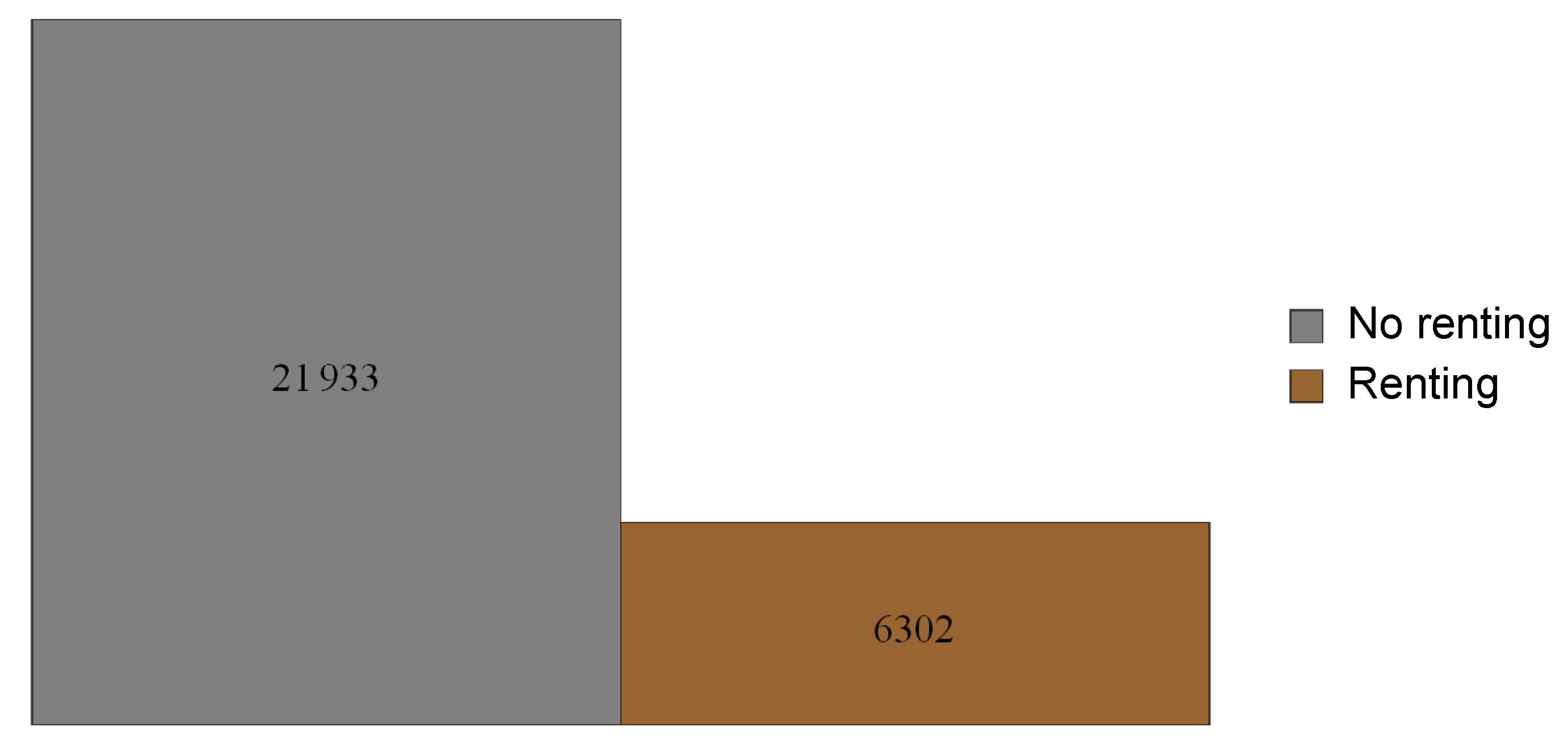
| Renting | 0 | 1 | 0.223 | — |
| (number of observations) | (21,933) | (6302) | ||
| General variables | ||||
| Origin spent | 0.52 | 1988.76 | 99.919 | 64.413 |
| Destination spent | 0 | 500 | 40.679 | 37.105 |
| Nights | 1 | 180 | 8.917 | 7.238 |
| Previous visits | 0 | 1 | 0.767 | — |
| Accommodation | 0 | 1 | 0.548 | — |
| Party | 0 | 1 | 0.818 | — |
| Booking | 0 | 1 | 0.985 | — |
| Low cost | 0 | 1 | 0.518 | — |
| Season: | ||||
| Jan-May | 0 | 1 | 0.371 | — |
| Jun-Sep | 0 | 1 | 0.295 | — |
| Oct-Dec | 0 | 1 | 0.333 | — |
| Trip motivation variables | ||||
| SunBeach | 0 | 1 | 0.903 | — |
| Holiday | 0 | 1 | 0.939 | — |
| Socio-economic variables | ||||
| Age | 16 | 92 | 44.827 | 14.275 |
| Gender | 0 | 1 | 0.495 | — |
| Income | 1 | 7 | 3.540 | 2.038 |
| Job | 0 | 1 | 0.818 | — |
| Nationality: | ||||
| German | 0 | 1 | 0.173 | — |
| British | 0 | 1 | 0.276 | — |
| Spanish | 0 | 1 | 0.185 | — |
| Nordic | 0 | 1 | 0.099 | — |
| Other | 0 | 1 | 0.267 | — |
| Observations | 28,235 |
| Frequentist | Asymmetric Bayesian | |||||||
|---|---|---|---|---|---|---|---|---|
| Variables | Robust sd | p-Value | ME | sd | MC Error | ME | ||
| Origin spending | −0.004 | 3 × 10 | 0.000 | −6.4 × 10 | −3.246 | 0.312 | 0.022 | −0.002 |
| Destination spending | 0.004 | 4 × 10 | 0.000 | 6.4 × 10 | 1.791 | 0.187 | 0.013 | 9.9 × 10 |
| Nights | 0.008 | 0.002 | 0.000 | 1.3 × 10 | 0.698 | 0.184 | 0.010 | 3.5 × 10 |
| Repeat | −0.002 | 0.035 | 0.958 | −3.2 × 10 | −0.121 | 0.449 | 0.034 | −6.9 × 10 |
| Accommodation | −0.100 | 0.033 | 0.001 | -0.016 | −1.422 | 0.434 | 0.029 | −8.03 × 10 |
| Party | 0.591 | 0.045 | 0.000 | 0.087 | 7.383 | 0.727 | 0.066 | 0.004 |
| Booking | 0.470 | 0.143 | 0.001 | 0.067 | 4.734 | 1.462 | 0.144 | 0.002 |
| Low cost | 0.217 | 0.031 | 0.000 | 0.035 | 2.775 | 0.414 | 0.030 | 0.001 |
| Jan-May | −0.098 | 0.036 | 0.007 | −0.016 | −1.285 | 0.456 | 0.029 | −7.3 × 10 |
| Jun-Sep | −0.039 | 0.037 | 0.289 | −0.006 | −0.507 | 0.472 | 0.031 | −2.9 × 10 |
| SunBeach | −0.069 | 0.054 | 0.198 | −0.011 | −0.968 | 0.635 | 0.057 | −5.6 × 10 |
| Holiday | 0.977 | 0.083 | 0.000 | 0.125 | 12.33 | 1.119 | 0.108 | 0.006 |
| Age | −0.004 | 0.001 | 0.000 | −6.4 × 10 | −0.823 | 0.226 | 0.013 | −4.5 × 10 |
| Gender | 0.141 | 0.030 | 0.000 | 4.7 × 10 | 1.760 | 0.387 | 0.024 | 0.001 |
| Income | 0.072 | 0.008 | 0.000 | 0.012 | 1.865 | 0.241 | 0.016 | 9.4 × 10 |
| Job | 0.217 | 0.044 | 0.000 | 0.034 | 2.791 | 0.601 | 0.052 | 0.0015 |
| German | 0.142 | 0.044 | 0.001 | 0.023 | 1.806 | 0.565 | 0.038 | 0.001 |
| British | −1.053 | 0.044 | 0.000 | −0.150 | −13.770 | 0.977 | 0.087 | −0.007 |
| Spanish | 0.469 | 0.044 | 0.000 | 0.081 | 5.881 | 0.688 | 0.056 | 0.003 |
| Nordic | −0.767 | 0.629 | 0.000 | −0.106 | −9.944 | 1.001 | 0.074 | −0.005 |
| Intercept | −3.079 | 0.183 | 0.000 | −58.330 | 3.765 | 3.765 | ||
| 29.090 | 1.767 | 0.176 | ||||||
| Observations | 28,235 | 28,235 | ||||||
| % Correct fit | 77.61 | 99.99 | ||||||
| DIC | 27,862.584 | 4647.380 | ||||||
| AIC | 27,904.584 | 2369.000 | ||||||
| BIC | 28,077.798 | 2550.000 | ||||||
Publisher’s Note: MDPI stays neutral with regard to jurisdictional claims in published maps and institutional affiliations. |
© 2021 by the authors. Licensee MDPI, Basel, Switzerland. This article is an open access article distributed under the terms and conditions of the Creative Commons Attribution (CC BY) license (https://creativecommons.org/licenses/by/4.0/).
Share and Cite
Dávila-Cárdenes, N.; Pérez-Sánchez, J.M.; Gómez-Déniz, E.; Boza-Chirino, J. Skewed Binary Regression to Study Rental Cars by Tourists in the Canary Islands. J. Risk Financial Manag. 2021, 14, 541. https://0-doi-org.brum.beds.ac.uk/10.3390/jrfm14110541
Dávila-Cárdenes N, Pérez-Sánchez JM, Gómez-Déniz E, Boza-Chirino J. Skewed Binary Regression to Study Rental Cars by Tourists in the Canary Islands. Journal of Risk and Financial Management. 2021; 14(11):541. https://0-doi-org.brum.beds.ac.uk/10.3390/jrfm14110541
Chicago/Turabian StyleDávila-Cárdenes, Nancy, José María Pérez-Sánchez, Emilio Gómez-Déniz, and José Boza-Chirino. 2021. "Skewed Binary Regression to Study Rental Cars by Tourists in the Canary Islands" Journal of Risk and Financial Management 14, no. 11: 541. https://0-doi-org.brum.beds.ac.uk/10.3390/jrfm14110541