
Short-Term Impact of COVID-19 on Indian Stock Market


1
Madras School of Economics (MSE), Gandhi Mandapam Road, Kottur, Chennai 600025, India
2
Department of Finance, St. Petersburg School of Economics and Management, National Research University Higher School of Economics, Kantemirovskaya St. 3A, 194100 Saint Petersburg, Russia
*
Author to whom correspondence should be addressed.
J. Risk Financial Manag. 2021, 14(11), 558; https://0-doi-org.brum.beds.ac.uk/10.3390/jrfm14110558
Submission received: 27 September 2021
/
Revised: 8 November 2021
/
Accepted: 16 November 2021
/
Published: 18 November 2021
(This article belongs to the Special Issue Financial Markets—The Response in Crisis Moments)
Abstract
:The onset of the COVID-19 pandemic and lockdown announcements by governments have created uncertainty in business operations globally. For the first time, a health shock has impacted the stock markets forcefully. India, one of the major emerging markets, has witnessed a massive fall of around 40% in its major stock indices’ value. Therefore, we examined the short-term impact of the pandemic on the Indian stock market’s major index (NIFTY50) and its constituent sectors. For our analysis, we used three different models (constant return model, market model, and market-adjusted model) of event study methodology. Our results are heterogeneous and largely depend on the sectors. All the sectors were impacted temporarily, yet the financial sector faced the worst. Sectors like pharma, consumer goods, and IT had positive or limited impacts. We discuss the potential explanations for the same. These results may be useful for investors in safeguarding equity portfolios from unforeseen shocks and making better investment decisions to avoid large, unexpected losses.
1. Introduction
The financial system plays an important role in the global economy (Maiti et al. 2021). Systemic events cause widespread financial instability that disrupts the functioning of the financial system, which in turn creates shocks in the real economy (Duca and Peltonen 2013; Thanh et al. 2020). Systemic shocks or contagious idiosyncratic shocks lead to systemic crises, thus severely impairing the financial system and destabilising the economy (De Bandt and Hartmann 2000). Therefore, academia and policymakers closely follow the stability and soundness of an economy’s financial system.
An important constituent of the Indian financial system is the Indian stock market. India is one of the emerging economies. It follows an open economy policy and is one of the largest recipients of FDI (foreign direct investment) in major sectors. Over the past two decades, the Indian stock market has shown impressive growth, especially in terms of turnover rate, market capitalisation, and the number of listed companies. Having said that, globalisation also makes the country vulnerable to various global risks (Maiti 2020). For example, the recent developments in asset markets depend on international capital flows. Therefore, any reversal of these flows creates an adverse impact on future capital raising and asset valuations. According to the Global Risk Report published by the World Economic Forum (2018), policymakers and entrepreneurs, especially in the emerging economies, are not well prepared to face serious economic or financial turmoil. Therefore, analysing the impact of major events on the emerging economies like India is very important. The impact of any such risks is immediately reflected in stock markets.
Stock markets are highly volatile and often spread the risks caused by systemic events such as asset bubbles, macro imbalances, negative externalities, correlated exposures, information disruptions and contagions, etc., to the existing economic and financial markets using various channels. In general, investors in the stock market are regarded as poor Bayesian decision-makers and evidence shows that they overreact to recent information. Investor optimism leads to a reduction in earnings volatility, whereas investor pessimism causes an increase in earnings volatility. As a result, stock prices deviate from their underlying fundamental value (De Bandt and Thaler 1987; Lee et al. 2002). Having said that, the decisions on the financial markets are ruled by “collective belief.” Investors pay attention to the way a collective opinion is formed and react accordingly (Orleéan 2004, 2008). This results in herding and stock prices deviating from their underlying fundamental value. Therefore, the investor overreaction hypothesis (IOH) challenges the efficiency of markets. Studying the effect of various unanticipated events on the stock price is important. One such unanticipated event that recently crashed the world economy and created adverse impact in the global stock market is the COVID-19 pandemic.
COVID-19, or coronavirus disease 2019, caused by the SARS-CoV-2 virus, was first detected in Wuhan, China. Consequently, numerous cases were traced around the world and the World Health Organization declared it a global pandemic on 11 March 2020. Unlike in developed economies, emerging markets such as India with (i) relatively poor public health infrastructure, (ii) a distressed and burdened banking sector and bond markets, and (iii) slowdown in economic growth face extreme difficulties while the effects of the pandemic unfold. On 24 March 2020, a nationwide lockdown was announced in India to reduce the adverse consequences. Such social distancing measures and restrictions on transportation negatively impacted firms’ productivity via increasing operation costs, decreasing revenue, and cash flow challenges. The usual consumption pattern was affected due to the growing panic among consumers. All these led to market abnormality (Bora and Basistha 2021). NIFTY rapidly dropped 40% of its market value compared to its value at the start of the year. The sudden fall in the indices affected the individual portfolios of investors. However, active retail investors found this as an opportunity to time the market, invest, and earn considerable returns. A total of 10 million new demat accounts were opened in 2020 owing to the low cost of trades and an industry-wide shift to online trading1. Reports show that the MSCI World Index, which includes stocks from 23 developed countries and 24 emerging markets, lost 10.7% of its value between 23 January and 6 March 2020. The outbreak of COVID-19 affected economies globally and India was one of them. The pandemic created an unprecedented global shock, increasing the financial market volatility. The global economy crashed, unemployment increased, and oil prices fell during the initial stage but increased significantly at the later phase (Alam et al. 2020). Since the Indian stock market is well integrated and responds to global situations, elucidating the impact of COVID-19 on the Indian stock market is important. One such method to measure this impact is the use of event study methodology, introduced by Fama et al. (1969).
Event study methodology is incorporated into investments and accounting to assess the volatility of stock prices and to check whether an event can affect the performance of various stocks and produce abnormal returns. Generally, event analysis is used (1) to test whether any new information is efficiently incorporated by the markets and (2) to examine the effect of an event on the security holder’s wealth, assuming that the market efficient hypothesis holds true, at least with respect to the information available to the public (Binder 1998). The important characteristics of event analysis is that it does not take into account the issues of stationarity and seasonality in a time series, whereas autoregressive moving average (ARMA) models are only applied to stationary time series and are not applicable directly on a seasonal time series. This method also examines whether the correlation between the variables is positive or negative. Hence, event study analysis is widely used in finance literature. Numerous studies have examined the effect of emergencies on stock price using event study analysis, such as the impact of terrorist attacks (Arin et al. 2008; Drakos 2010), political events (Beaulieu et al. 2006; Bash and Alsaifi 2019), nuclear disasters (Kawashima and Takeda 2012), the severe acute respiratory syndrome (SARS) pandemic disease outbreak (Chen et al. 2007), epidemics (Chen et al. 2007; Ichev and Marinč 2018; Salisu and Vo 2020), etc.
The objective of this study is to examine the impact of the global pandemic in the Indian stock market. The National Stock Exchange (NSE), one of the two major stock exchanges in India, is globally the third largest stock exchange in terms of the number of equity trades and has the world’s largest derivatives by volume. Therefore, this paper studies the effect of the COVID-19 outbreak by employing event study methodology on the NIFTY50 index and its constituents. The NIFTY50 index is the benchmark index of the NSE. One of the salient features of the paper is examining the effect of the pandemic on the major constituent sectors of the NIFTY50 index—financial services, consumer goods, IT, and pharma.
2. Literature Review
The COVID-19 pandemic increased uncertainty and risk around the globe and affected both developed and emerging economies such as the United States, Italy, Spain, Brazil, and India. Existing studies recorded diversified results. Ozili and Arun (2020) used major government policies such as public health measures, restrictive measures, social distancing policies, and fiscal monetary policies to elucidate the impact of COVID-19 on the global economy. According to them, higher fiscal policy and restriction on movement had a negative impact on the level of economic activities. In line with the results, Adda (2016) employed quasi-experimental variation and showed that the travel restrictions during a viral disease outbreak decreased the earnings and adversely impacted the economy. In addition, Gormsen and Koijen (2020) documented that the lock-down in Italy due to the COVID-19 pandemic caused a downward trend in the GDP growth and dividends of US and European countries. Similarly, Zhang et al. (2020) examined the top 10 COVID-19-infected countries using a simple statistical analysis method and suggested that the pandemic created greater risk and uncertainty in the global market. This is in line with the conclusions drawn by Baker et al. (2020), who showed that the market swings due to COVID-19 were extremely high when compared with the times of SARS, swine flu, MERS, Ebola and bird flu. Similarly, Liu et al. (2020) employed event study methodology, analysing 21 leading stock exchanges and concluding that the COVID-19 outbreak had a significant negative impact on the stock markets of all affected countries, with Asia recording a greater decrease in terms of abnormal returns. This explanation is consistent with the findings of Harjoto et al. (2021), who used event analysis to show the strong negative impact of COVID-19 on the global markets, especially emerging markets and small firms. According to this study, large firms and the US stock market recorded positive abnormal returns compared to the other emerging market economies. Adding to this result, Ramelli and Wagner (2020) analysed the international trade and financial policies of individual firms and concluded that internationally oriented US firms, especially those with exposure to the Chinese market, faced adverse impacts. Several studies focused on analysing individual market economies. For example, Al-Awadhi et al. (2020) used a panel regression approach to examine the impact of the global pandemic on the different sectors of the Chinese stock market. According to this study, high market capitalisation stocks were adversely affected, but the performance of the information technology and pharma sectors were relatively better. According to Topcu and Gulal (2020), Asian emerging economies were more affected by the outbreak than European emerging economies. This increased the rate of interest on the sovereign debt of emerging markets (Goldberg and Reed 2020).
Various methods were employed by different studies to address the impact of the COVID-19 outbreak in different stock markets and financial assets (Maiti et al. 2020; Maiti 2021; Vukovic et al. 2021). Cepoi (2020) employed panel quantile regression and Bora and Basistha (2021) used a generalised autoregressive conditional heteroscedasticity model to gauge the impacts. One such method popularly used to measure the impact of an unprecedented event is event study methodology.
Over the years, event study methodology has evolved with several advancements. Event analysis was first used by Dolley (1933) to examine the impact of stock splits on stock price. By the 1960s, several researchers (Myers and Bakay 1948; Barker 1956; Ashley 1962) had contributed to this methodology. Nevertheless, Ball and Brown (1968) and Fama et al. (1969) are regarded as the pioneers in the event study methodology. The former worked on the information content of earnings, whereas the latter, popularly known as the event study of FFJR, designed a classic market model to elucidate the effect of stock splits after the removal of the simultaneous dividend increase effect (Mackinlay 1997). The market model was patterned after the development of the capital asset pricing model (Sharpe 1964; Corrado 2011). In the earlier days, around the time of an event, the market model was mainly used to calculate the cumulative mean abnormal returns. The number of papers contributing to event study in the 1980s increased. In the late 1990s, various sophisticated methods to estimate abnormal returns were introduced, especially for long-run event studies. Windows of one year or more are termed “long-horizon.” The advancement was mainly due to various developments in the asset pricing literature, such as the three-factor model by Fama and French (1995) and the use of daily or intraday data instead of monthly data (Mackinlay 1997). However, long-run events lack reliability and long-horizon abnormal returns are precarious (Brown and Warner 1980; Lyon et al. 1999). Long-horizon tests have low power and are subjected to joint-test problems (Kothari and Warner 2006). According to Fama (1991), short-run tests give the “cleanest evidence on efficiency.” Therefore, this study employed short-horizon event study methodologies, as they are relatively trouble-free and straightforward.
The event study method is a tool to assess the impact of an unanticipated event on the firm value. Assuming rationality in the market, the effect of an event is immediately reflected in the share price (Mackinlay 1997). In stock markets, unexpected events affect investor sentiment, which in turn impacts their decision-making ability. This results in changes in the stock price (He et al. 2020). In the past, several studies have contributed to the literature on event analysis but only a few studies analysed the impact of a health crisis on the stock market. Among the very few, most of the studies concentrated on influenza and the severe acute respiratory syndrome (SARS) pandemic disease outbreak (Chen et al. 2007; Goh and Law 2002). Recently, one such health crisis that has had an adverse and sustained impact on the global economy is the outbreak of COVID-19 (Iyke 2020).
Very few studies have contributed to analysing the impact of COVID-19 on the Indian stock market using event study methodology. Therefore, the motivation of this study is to contribute to the growing literature by constructing three different models—the constant return model, the market adjusted model, and the market model. Some studies addressed the impact of the pandemic on different sectors of various international stock markets (Ramelli and Wagner 2020; He et al. 2020; Albuquerque et al. 2020). However, evidence pertaining to the Indian stock market is scarce. This paper attempts to fill this gap by analysing the impact of COVID-19 on different sectors of the NIFTY50 index. The overall objective of the paper is to test whether the onset of the COVID-19 pandemic produced abnormal returns by analysing the constituents of the NIFTY50 index using event study methodology.
3. Data and Methodology
3.1. Data
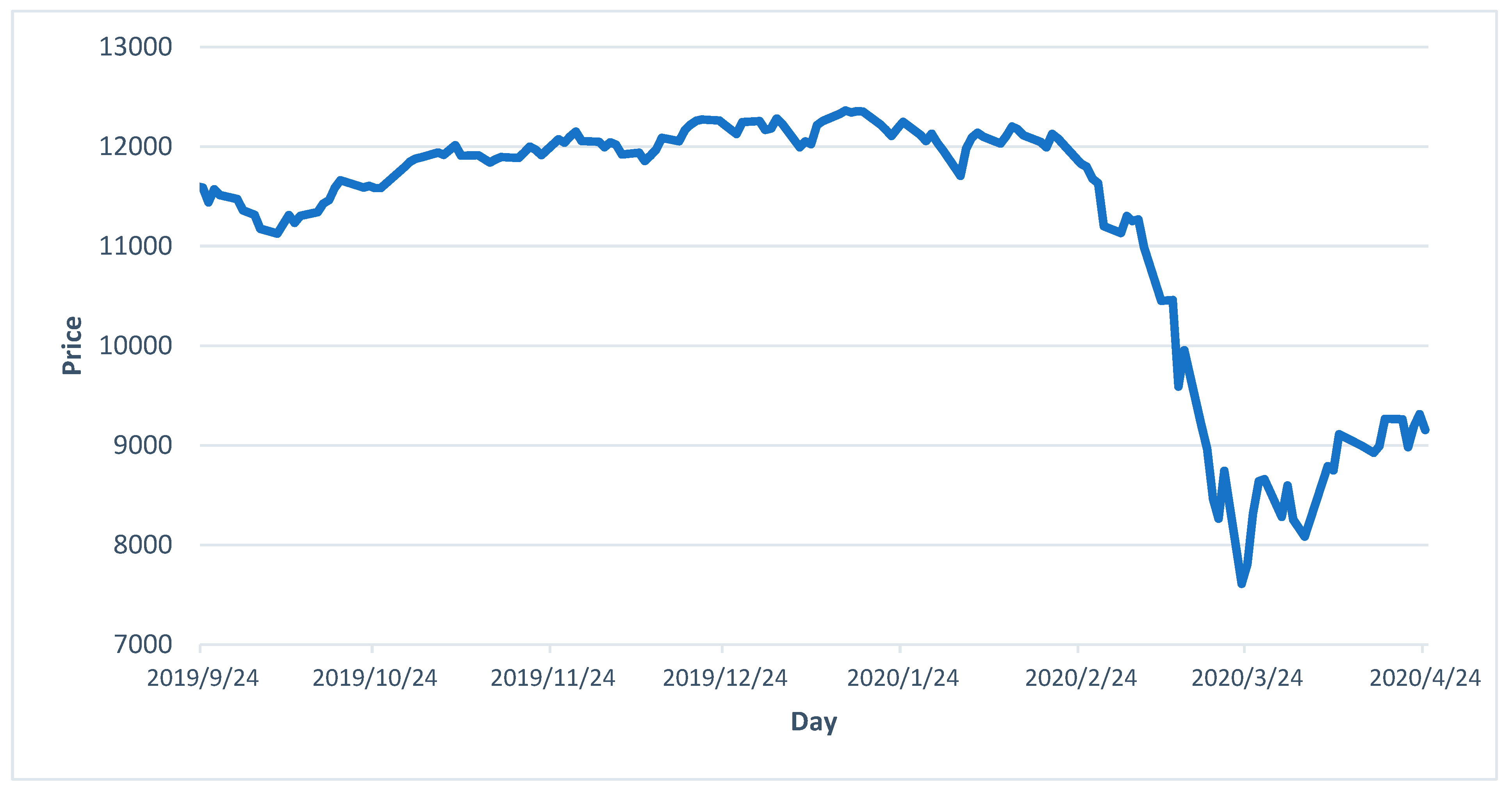
The study aims to check the impact of the COVID-19 outbreak on the Indian stock market in March 2020. Stock prices adjusted for stock splits and dividends were taken from the Yahoo Finance and CMIE Prowess databases. Daily security prices were considered for the analysis. The NIFTY50 index is the float-adjusted market-capitalisation-weighted index consisting of 50 stocks of blue-chip companies and represents about 65% of the NSE’s float-adjusted market capitalisation. The NIFTY50 index was chosen as the proxy for market returns. The analysis was carried out on the constituents of the NIFTY50 index. Figure 1 shows the movement of the index during the onset of the pandemic. It exhibits that the market fell by about 15–17% in March during the onset of the pandemic in India. The month of April was relatively better as the market tried to recover from the lows of March and showed an upward trend.
3.2. Methodology
The effect of an event is immediately realised in the stock price, unlike other productivity-related measures that require months of observation. An event’s impact is assessed by measuring abnormal returns. Event study methodology helps to check whether such unanticipated events caused abnormal returns. An abnormal return is defined as the difference between the actual ex-post security’s return over the event window and the expected normal return (Mackinlay 1997). Three models—the constant mean return model, the market adjusted model, and the market model were used to measure the associated abnormal returns.
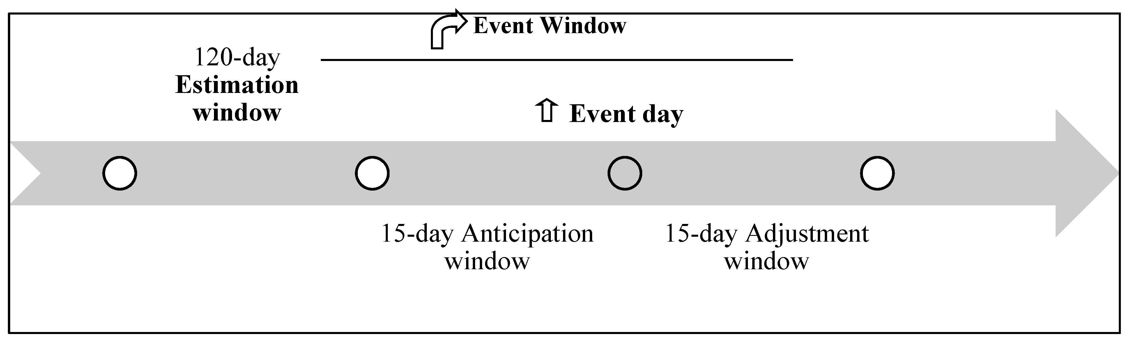
Step 1: Define event window and estimation window
The initial step in an event analysis is to define the event of interest and the event window. The Government of India imposed a nationwide lockdown on the evening of 24 March 2020. Since the impact of that announcement on the stock market is realised the next day, 25 March 2020 was the event of interest. The event window is the time period during which the security prices are impacted by a particular event. The event window consists of two components—the anticipation window and the adjustment window. The day of impact or the event day is set as day 0. The 15 days prior to the event are called the anticipation window and the 15 days after the event constitute the adjustment window. This study deviated from the usual practice of selecting a 10-day anticipation and adjustment window. Since the virus is throwing surprises daily and is still in the stage of being discovered around the globe, a 15-day event window helps capture investor behaviour in a prominent manner. The next step was to define the estimation window. The estimation window is a pre-decided time frame before the occurrence of an event. The estimation period is day −135, −16, i.e., it ends 15 days prior to the event day and covers a period of 120 trading days. Figure 1 depicts the timeline of the event analysis. In order to eliminate potential biases, the estimation period is separated from the event period (Hendricks and Singhal 2003).
Unlike a short event window (at most 1 month prior and 1 month after), a long event window (i) decreases the power of the test statistics, (ii) leads to confounding effects, and (iii) results in false conclusions (McWilliams and Siegel 1997). Since event analysis depends on forecasting, the results’ accuracy decreases over time. The probability of any other event influencing the stock price and creating noise is relatively higher in long periods. Therefore, a short event window was considered for the analysis. Figure 2 shows the timeline of the event window considered in our analysis. In this work, we considered an event window of 15 days prior and 15 days after to capture a better picture of the COVID-19 pandemic-related impact, as this was not a single-day event. Instead, the event was spread over days as the COVID-19 numbers increased every day. Therefore, to capture a better picture, we increased the size of the event window by 5 more days (usually 10 days before and after the window are considered for a single-day event).
Step 2: Calculate abnormal returns
The reaction of the stock market to the arrival of new information is reflected by abnormal returns (McWilliams and Siegel 1997). It is assumed that the asset returns are iid (independently and identically distributed) through time and jointly multivariate normal. The three different models used to calculate abnormal returns are outlined below.
3.2.1. Constant Mean Return Model
The constant mean return model is the simplest model but yields the same results as other sophisticated models (Brown and Warner 1980, 1985). It only takes into account the average return of the stock and does not adjust for index returns. Hence, this model tends to give inflated abnormal returns. An abnormal return from the constant mean return model is given below in Equation (1).
where ξi,t is the abnormal return with E[ξi,t] = 0 and Var[ξi,t] = σξ,i2, Ri,t is the actual return on stock i on each day t of the estimation period, Xt is the conditioning information at time t, and E(Ri,t|Xt) = μi is the average return of the stock in the estimation window.
ξi,t = Ri,t − E(Ri,t|Xt)
3.2.2. Market Model
The market model isolates the impact of market-related factors and controls systematic risk. It is considered a benchmark model to calculate normal return. This model is preferred to the constant mean return model, as it removes the excess returns due to market return variation, thus reducing the variance of abnormal return (Mackinlay 1997). Expected return/normal return from the market model is given below in Equation (2).
where Ri,t is the actual return on stock i on each day t of the estimation period. Similarly, Rm,t is the market return on each day t. The estimated alpha and beta are obtained from the estimation period. The ordinary least square method over a period of 120 estimation days is employed to estimate αi and βi.
E(Ri,t) = αi + βi x Rm,t
The abnormal return for a market model is characterised in Equation (3).
where E(Ri,t) is the expected return (Equation (2)). The abnormal return (ξi,t) with E[ξi,t] = 0 and Var[ξi,t] = σξ,i2 is the difference between the actual daily return of the stock i and the estimated normal return of stock i on day t.
ξi,t = Ri,t − E(Ri,t)
3.2.3. Market Adjusted Model
The market adjusted model is the constrained market model where αi = 0 and βi = 1 (Mackinlay 1997). The market adjusted model takes the index returns into account. Hence, this model does not give inflated abnormal returns. Abnormal returns from the market adjusted model are measured as in Equation (4).
where Rit is the actual return on stock i on each day t of the estimation period and RIi,t is the actual return of the index on each day t of the estimation period.
ξi,t = Ri,t − RIi,t
Step 3: Calculate average abnormal returns
The daily average abnormal return (AAR) is given by:
where N is the number of firms for which the average abnormal returns are being calculated.
The t-test is employed to test the significance:
Significance is tested for the 3 models in the event period.
Step 4: State the hypothesis
The null and alternative hypotheses are:
Null Hypothesis (H0): Average abnormal returns in the event window are not statistically significant.
Alternate Hypothesis (H1): Average abnormal returns in the event window are statistically significant.
4. Results and Discussions
4.1. Average Abnormal Returns from NIFTY50 Index Components
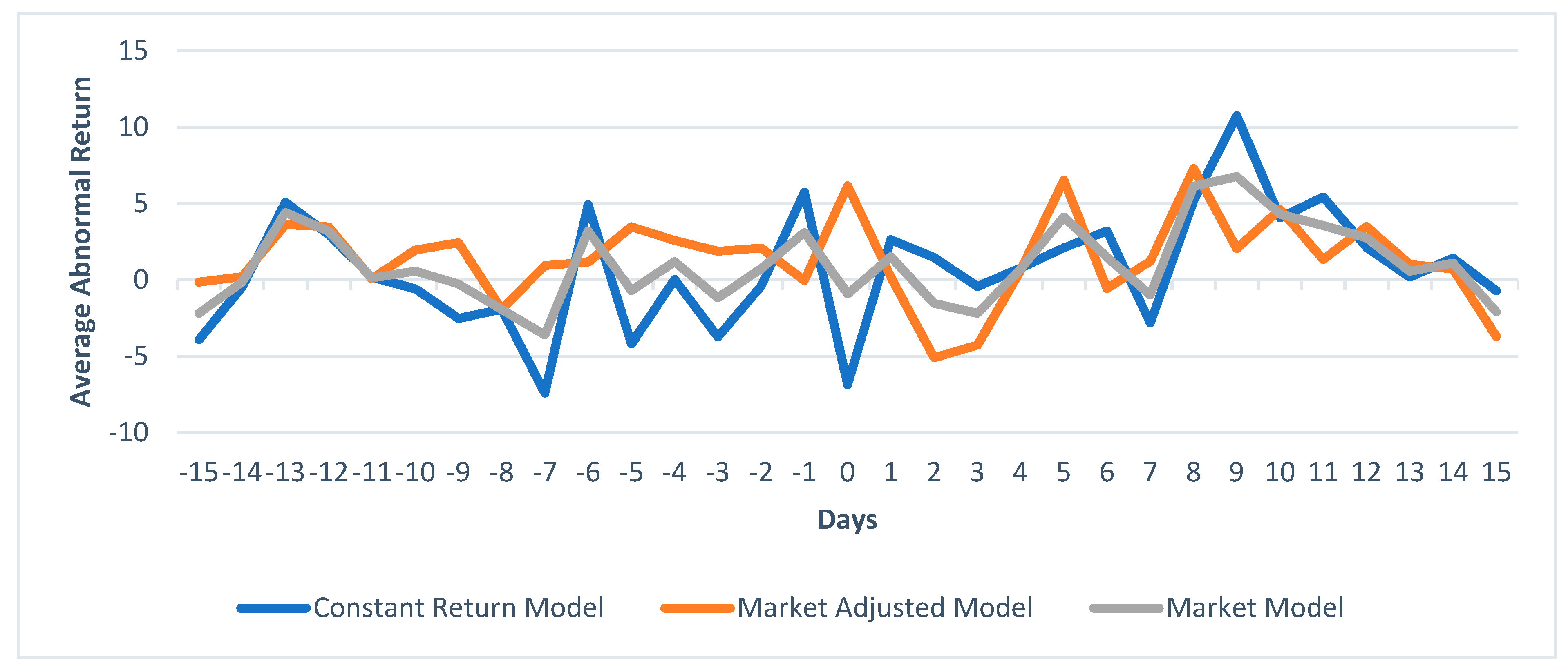
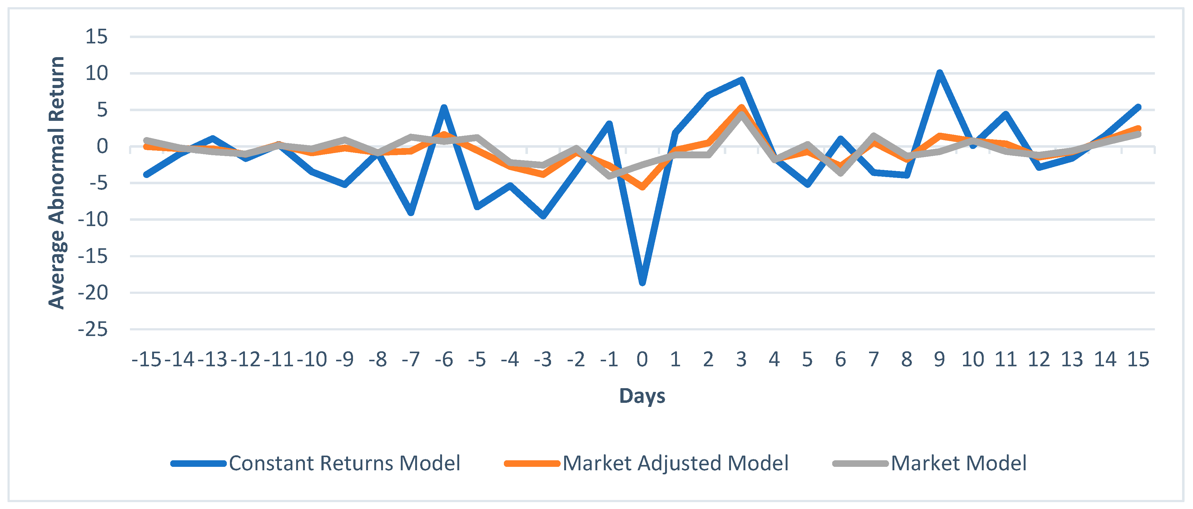
Unlike the US, the stock markets in India reacted even before the actual outbreak of COVID-19 at its peak in India owing to the knowledge from the experience of other countries (Verma et al. 2021). Therefore, this paper analyses the initial stage of the outbreak. The average abnormal returns for 50 stocks constituting the NIFTY50 index were calculated using the three different models—the constant return model, the market model and the market adjusted model. With a 5% significance level, the t-test was employed to test the significance. AAR was calculated for 30 days in the event window and is tabulated in Table 1 and Table 2. Table 1 represents the results of the constant return model. It exhibits that, on the day of the event, i.e., day 0, there was a significant negative mean abnormal return of 12.8%. The median AAR on the day of the event was −12.9%. Two days before and after the event, the AAR significantly differed from 0. Table 2 represents the results of the market model and market adjusted model. It shows that on the event day, the AARs of both models were not statistically significant. The null hypothesis cannot be rejected and the abnormal return on the event day was not statistically significant. However, a significant negative abnormal return two days before and after the event was also recorded. The abnormal return in each sector was analysed to elucidate the presence of positive abnormal returns on the event day.
From Table 1 and Table 2, we observed that some days did record significant AARs before and after the event. Firms with lower flexibility and high operating leverage faced adverse impacts. Since the components of NIFTY50 are blue-chip companies, firms with low operating leverage, more scalable operations, and greater operational flexibility suffered less loss in market value (Verma et al. 2021). Therefore, the AARs calculated from the market model and market adjusted model during the 30 days of the event window ranged only from −1.69 to 1.70 and from −1.72 to 1.69, respectively. Nevertheless, the analysis of the individual sectors helps identify the most affected sectors.
4.2. Impact of the Pandemic in Different Sectors of the NIFTY50 Index
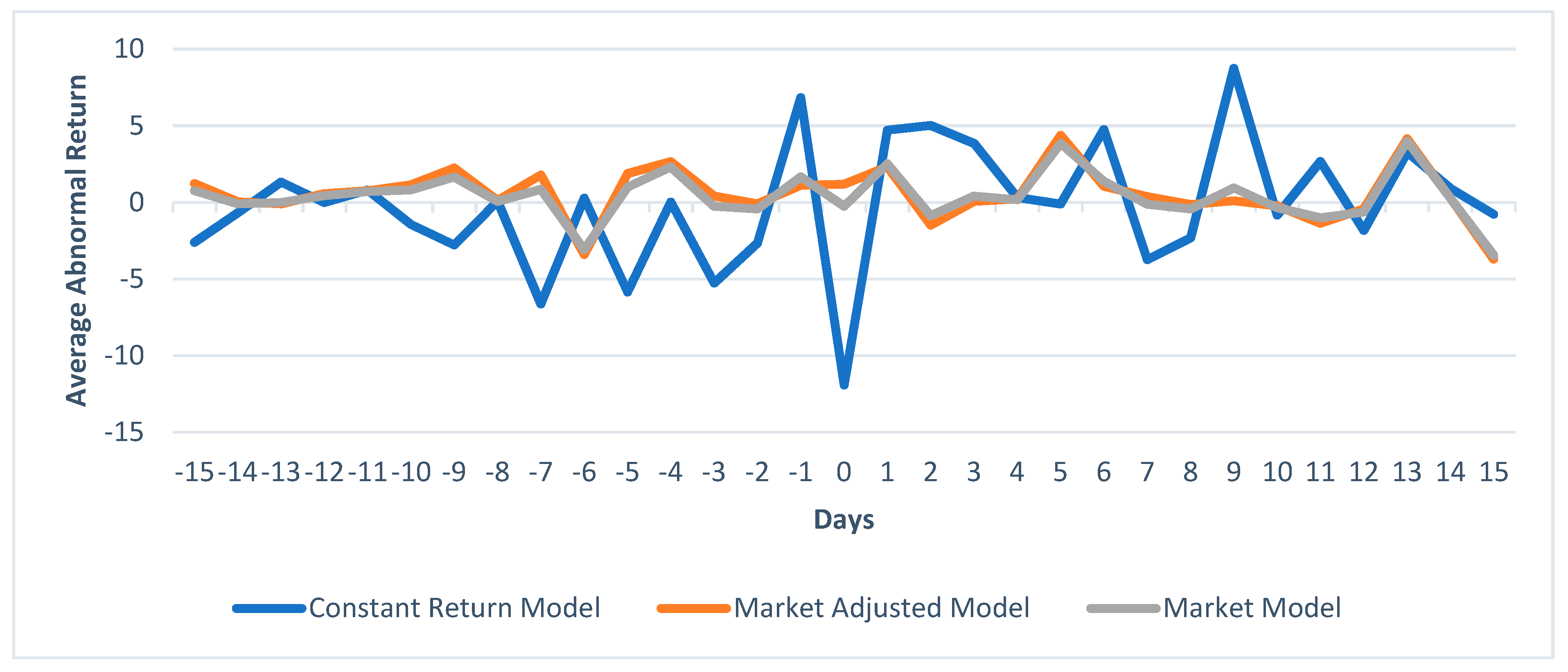
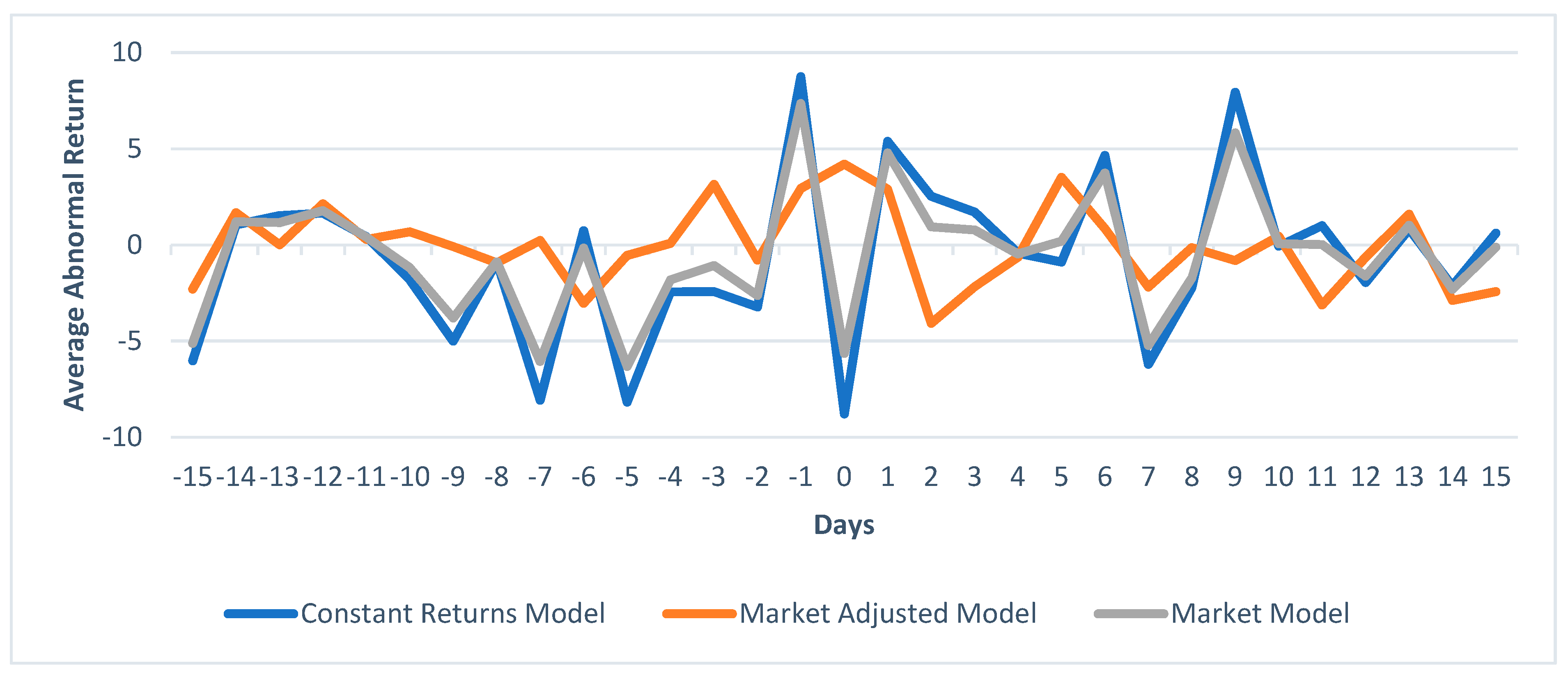
The NIFTY50 index consists of 13 different sectors—automobile, cement and cement products, construction, consumer goods, fertilisers and pesticides, financial services, IT, metals, oil and gas, pharma, power, and services. Figure 3, Figure 4, Figure 5 and Figure 6 show the average abnormal returns from the event window of four—pharma, consumer goods, financial services, and the IT sector, respectively. Since the financial services sector had the highest weightage (22%) in the index followed by consumer goods (14%), the automobile sector (12%), and IT (10%)2, these sectors were included in the analysis. When there is a change in the economic environment of a particular sector, the operating conditions of the firms in that sector are highly correlated (Moskowitz and Grinblatt 1999). Since the onset of pandemic had a direct impact on pharmaceutical companies, the pharma sector was included in the analysis.
From the graphs, all the sectors included in the graphs recorded the highest positive ARR on the ninth day after the event owing to the reports of positive trial results on experimental virus treatment3. Owing to the onset of the COVID-19 pandemic, it is evident that the pharma sector has to lead the way by producing the requisite set of drugs and vaccines to control and thereby reduce its adverse impact. On the day of the event, when the constant return model showed an AAR of about −6%, the market adjusted model showed a positive AAR of the same quantum. Pharma stocks did not fall as much as the index and the shares from this sector were long, as investors expected an upward growth in this sector in the near future. Certain pharma stocks recorded positive returns on the same day when the index fell by about 12%. Figure 3 records the AAR obtained from the stocks included in the pharma sector of the NIFTY50 index. On the event day, the constant return model recorded a negative ARR, whereas the market adjusted model recorded a positive ARR. Even though the first and second day after the event recorded a downward trend in AAR, the aftermath of the event did record a positive AAR. After the event day, all the models showed fluctuating AAR. This is similar to the results obtained by Ramelli and Wagner (2020), who documented that the pandemic had a huge impact on the pharmaceutical companies of the US market.
Similarly, Figure 4 highlights that the market adjusted model recorded positive returns for the consumer goods sector. Even after the adverse impacts of the lockdown and the prevailing uncertainties, the consumption stocks did not see a sharp decline. This is because (i) essential commodities are inelastic and their demand and supply would not decline even under these circumstances, and (ii) the consumer sector demonstrated low operational fragility and the market value did not face a severe blow during the crisis (Verma et al. 2021).
However, the financial services sector, which accounted for 22% weight in the index, was the worst hit. This sector was negatively impacted due to the anticipation of an increase in NPAs (non-performing assets) in the future. Since a nationwide lockdown was introduced, the revenues of the firms were expected to fall. Investors also expected defaults in the personal loan segment. Therefore, an expected increase in the credit risk of corporate and retail clients led to negative sentiments4 and investors started selling shares in this sector. This was also proven by the negative AAR on the event day (see Figure 5).
Figure 6 shows that the IT sector had a deep negative AAR in the days prior to the event. Due to the uncertainty prevailing in the market owing to the performance of the stocks, a heavy FII (foreign institutional investor) sell-off was recorded before the event. However, the INR depreciated after the occurrence of the event. The IT sector is an exporter of services. With most of the clients based outside India, Indian IT companies were expected to earn greater revenues. Investors were positive about this sector and some IT stocks even gave positive returns on the day of the event. The IT sector also had relatively low fragility due to the benefits from work-from-home production arrangements. Such speculations led the IT sector to produce A positive AAR after the announcement.
Apart from these sectors, the automobile sector also faced adverse impacts. Demand for automobiles decreased due to less disposable income and subdued economic activity. Most of the raw materials and finished goods in the electronics sector are imported from China. The adverse impact on the Chinese economy disrupted the supply chain and due to the prevailing uncertainty in growth, the demand for white goods like electronics decreased. Lack of demand has an adverse impact on sectors irrespective of their economic nature. Evidence shows that capital intensive firms were relatively more vulnerable to the shocks. However, firms demonstrating greater supply chain fragility did not face a severe impact in their market value (Verma et al. 2021). Other sectors were also affected by the pandemic, with tourism and real estate falling under the category of worst affected industries. However, lockdowns and social distancing measures had a positive impact on the telecommunication sector (Ramelli and Wagner 2020). Overall, uncertainty prevailed and the sentiments were negative. This fuelled the sell-off in the Indian stock market. The results from the market adjusted model and the market model imply that relying on the constant return model may lead to spurious conclusions, as the latter produces inflated returns compared to the former models.
5. Conclusions
This study examined the impact of COVID-19 on the Indian stock market by gauging the presence of abnormal returns during the onset of the pandemic. We use three different event study methodologies, including the constant return model, the market adjusted model, and the market model, for our analysis. Abnormal returns were noticed on many days before and after the occurrence of the event. After the announcement of complete lockdown, all the models showed consistently positive AARs on most of the days. Furthermore, we conducted sectoral analysis to understand the impact of the COVID-19 pandemic on individual sectors. Overall, we found that COVID-19 has increased the risk in the stock market. However, our results are heterogeneous and largely depend on the sectors. The findings are in line with Guru and Das (2021) and Shankar and Dubey (2021). All the sectors were impacted temporarily, but the financial sector faced the worst. Sectors like pharma, consumer goods, and IT had positive or limited impacts. Our result is similar to that of Bora and Basistha (2021), who found the pharma sector to be attractive during this health-related pandemic time.
Overall, this work indicates that a COVID-19-like shock would cause a sudden and large decline in stock market returns, and could pose an existential threat to the financial sector due to the possibility of extreme downturns in its stock prices. As the financial sector is the backbone of economic stability, policies should be formulated to mitigate mass panic during any pandemic. Looking at the connection between the dynamics of investors’ fear and financial markets, regulators should have effective mechanisms in place to deal with sudden extreme pessimism in the market. Furthermore, governments and central banks should communicate effectively and in a timely manner to help reduce the impact in the financial market (Al-Awadhi et al. 2020). The volatility of financial markets also depends on the speed with which extraordinary fiscal policies intervene to reduce the damages caused by COVID-19. Therefore, an increase in resources directed towards the health care system could also have a positive impact on reducing financial volatility. Furthermore, investors can learn from this kind of event to safeguard equity portfolios from unforeseen shocks and make better investment decisions to avoid large unexpected losses by choosing effective hedging or safe-haven strategies (SG and Kayal 2020; Conlon et al. 2020; Conlon and McGee 2020).
Author Contributions
Conceptualization, Y.V., R.V., P.K., and M.M.; methodology, Y.V., R.V., and P.K.; validation, Y.V., R.V., and P.K.; formal analysis, Y.V., R.V., and P.K.; writing—original draft preparation, Y.V., R.V., and P.K.; writing—review and editing, Y.V., R.V., P.K., and M.M. All authors have read and agreed to the published version of the manuscript.
Funding
This research received no external funding.
Data Availability Statement
The data presented in this study are available on reasonable request from P.K.
Conflicts of Interest
The authors declare no conflict of interest.
| 1 | https://www.moneycontrol.com/ (accessed on 1 February 2021). |
| 2 | National Stock Exchange. |
| 3 | Financial express. |
| 4 | KPMG Global: The impact of COVID-19 on the banking sector. |
References
- Adda, Jérôme. 2016. Economic activity and the spread of viral diseases: Evidence from high frequency data. The Quarterly Journal of Economics 131: 891–941. [Google Scholar] [CrossRef] [Green Version]
- Alam, Mohammad Noor, Md Shabbir Alam, and Kavita Chavali. 2020. Stock market response during COVID-19 lockdown period in India: An event study. The Journal of Asian Finance, Economics, and Business 7: 131–37. [Google Scholar] [CrossRef]
- Al-Awadhi, Abdullah M., Khaled Alsaifi, Ahmad Al-Awadhi, and Salah Alhammadi. 2020. Death and contagious infectious diseases: Impact of the COVID-19 virus on stock market returns. Journal of Behavioral and Experimental Finance 27: 100326. [Google Scholar] [CrossRef] [PubMed]
- Albuquerque, Rui, Yrjo Koskinen, Shuai Yang, and Chendi Zhang. 2020. Resiliency of environmental and social stocks: An analysis of the exogenous COVID-19 market crash. The Review of Corporate Finance Studies 9: 593–621. [Google Scholar] [CrossRef]
- Arin, K. Peren, Davide Ciferri, and Nicola Spagnolo. 2008. The price of terror: The effects of terrorism on stock market returns and volatility. Economics Letters 101: 164–67. [Google Scholar] [CrossRef]
- Ashley, John W. 1962. Stock prices and changes in earnings and dividends: Some empirical results. Journal of Political Economy 70: 82–85. [Google Scholar] [CrossRef]
- Baker, Scott R., Nicholas Bloom, Steven J Davis, Kyle Kost, Marco Sammon, and Tasaneeya Viratyosin. 2020. The unprecedented stock market reaction to COVID-19. The Review of Asset Pricing Studies 10: 742–58. [Google Scholar] [CrossRef]
- Ball, Ray, and Philip Brown. 1968. An empirical evaluation of accounting income numbers. Journal of Accounting Research, 159–78. [Google Scholar] [CrossRef] [Green Version]
- Barker, C. Austin. 1956. Effective stock splits. Harvard Business Review 34: 101–6. [Google Scholar]
- Bash, Ahmad, and Khaled Alsaifi. 2019. Fear from uncertainty: An event study of Khashoggi and stock market returns. Journal of Behavioral and Experimental Finance 23: 54–58. [Google Scholar] [CrossRef]
- Beaulieu, Marie-Claude, Jean-Claude Cosset, and Naceur Essaddam. 2006. Political uncertainty and stock market returns: Evidence from the 1995 Quebec referendum. Canadian Journal of Economics/Revue Canadienne D’économique 39: 621–42. [Google Scholar] [CrossRef]
- Binder, John. 1998. The event study methodology since 1969. Review of Quantitative Finance and Accounting 11: 111–37. [Google Scholar] [CrossRef]
- Bora, Debakshi, and Daisy Basistha. 2021. The outbreak of COVID-19 pandemic and its impact on stock market volatility: Evidence from a worst-affected economy. Journal of Public Affairs, e2623. [Google Scholar] [CrossRef] [PubMed]
- Brown, Stephen J., and Jerold B. Warner. 1980. Measuring security price performance. Journal of Financial Economics 8: 205–58. [Google Scholar] [CrossRef]
- Brown, Stephen J., and Jerold B. Warner. 1985. Using daily stock returns: The case of event studies. Journal of Financial Economics 14: 3–31. [Google Scholar] [CrossRef]
- Cepoi, Cosmin-Octavian. 2020. Asymmetric dependence between stock market returns and news during COVID-19 financial turmoil. Finance Research Letters 36: 101658. [Google Scholar] [CrossRef] [PubMed]
- Chen, Ming-Hsiang, SooCheong Shawn Jang, and Woo Gon Kim. 2007. The impact of the SARS outbreak on Taiwanese hotel stock performance: An event-study approach. International Journal of Hospitality Management 26: 200–12. [Google Scholar] [CrossRef] [PubMed]
- Conlon, Thomas, and Richard McGee. 2020. Safe haven or risky hazard? Bitcoin during the COVID-19 bear market. Finance Research Letters 35: 101607. [Google Scholar] [CrossRef]
- Conlon, Thomas, Shaen Corbet, and Richard J. McGee. 2020. Are cryptocurrencies a safe haven for equity markets? An international perspective from the COVID-19 pandemic. Research in International Business and Finance 54: 101248. [Google Scholar] [CrossRef]
- Corrado, Charles J. 2011. Event studies: A methodology review. Accounting & Finance 51: 207–34. [Google Scholar]
- De Bandt, Olivier, and Philipp Hartmann. 2000. Systemic Risk: A Survey. European Central Bank Working Paper No. 35. Available online: https://www.ecb.europa.eu/pub/pdf/scpwps/ecbwp035.pdf (accessed on 1 April 2021).
- De Bandt, Werner F. M., and Richard H. Thaler. 1987. Further evidence on investor overreaction and stockmarket sensitivity. Journal of Finance 42: 557–81. [Google Scholar] [CrossRef]
- Dolley, James C. 1933. Open market buying as a stimulant for the bond market. Journal of Political Economy 41: 513–29. [Google Scholar] [CrossRef]
- Drakos, Konstantinos. 2010. Terrorism activity, investor sentiment, and stock returns. Review of Financial Economics 19: 128–35. [Google Scholar] [CrossRef]
- Duca, Marco Lo, and Tuomas A. Peltonen. 2013. Assessing systemic risks and predicting systemic events. Journal of Banking & Finance 37: 2183–95. [Google Scholar]
- Fama, Eugene F. 1991. Time, salary, and incentive payoffs in labor contracts. Journal of Labor Economics 9: 25–4. [Google Scholar] [CrossRef]
- Fama, Eugene F., and Kenneth R. French. 1995. Size and book-to-market factors in earnings and returns. The Journal of Finance 50: 131–55. [Google Scholar] [CrossRef]
- Fama, Eugene F., Lawrence Fisher, Michael C. Jensen, and Richard Roll. 1969. The adjustment of stock prices to new information. International Economic Review 10: 1–21. [Google Scholar] [CrossRef]
- Goh, Carey, and Rob Law. 2002. Modeling and forecasting tourism demand for arrivals with stochastic nonstationary seasonality and intervention. Tourism Management 23: 499–510. [Google Scholar] [CrossRef]
- Goldberg, Pinelopi Koujianou, and Tristan Reed. 2020. The effects of the coronavirus pandemic in emerging market and developing economies: An optimistic preliminary account. Brookings Papers on Economic Activity 2020: 161–235. [Google Scholar] [CrossRef]
- Gormsen, Niels Joachim, and Ralph S. J. Koijen. 2020. Coronavirus: Impact on stock prices and growth expectations. The Review of Asset Pricing Studies 10: 574–97. [Google Scholar] [CrossRef]
- Guru, Biplab Kumar, and Amarendra Das. 2021. COVID-19 and uncertainty spillovers in Indian stock market. MethodsX 8: 101199. [Google Scholar] [CrossRef] [PubMed]
- Harjoto, Maretno Agus, Fabrizio Rossi, and John K. Paglia. 2021. COVID-19: Stock market reactions to the shock and the stimulus. Applied Economics Letters 28: 795–801. [Google Scholar] [CrossRef]
- He, Pinglin, Yulong Sun, Ying Zhang, and Tao Li. 2020. COVID–19′s impact on stock prices across different sectors—An event study based on the Chinese stock market. Emerging Markets Finance and Trade 56: 2198–212. [Google Scholar] [CrossRef]
- Hendricks, Kevin B., and Vinod R. Singhal. 2003. The effect of supply chain glitches on shareholder wealth. Journal of Operations Management 21: 501–22. [Google Scholar] [CrossRef]
- Ichev, Riste, and Matej Marinč. 2018. Stock prices and geographic proximity of information: Evidence from the Ebola outbreak. International Review of Financial Analysis 56: 153–66. [Google Scholar] [CrossRef]
- Iyke, Bernard Njindan. 2020. Economic policy uncertainty in times of COVID-19 pandemic. Asian Economics Letters 1: 17665. [Google Scholar]
- Kawashima, Shingo, and Fumiko Takeda. 2012. The effect of the Fukushima nuclear accident on stock prices of electric power utilities in Japan. Energy Economics 34: 2029–38. [Google Scholar] [CrossRef]
- Kothari, Sagar P., and Jerold B. Warner. 2006. Econometrics of event studies. In Handbook of Corporate Finance: Empirical Corporate Finance, Forthcoming (vol. A, ch. 1.). Edited by Espen Eckbo. Handbooks in Finance Series; Amsterdam: Elsevier. [Google Scholar]
- Lee, Wayne Y., Christine X. Jiang, and Daniel C. Indro. 2002. Stock market volatility, excess returns, and the role of investor sentiment. Journal of Banking & Finance 26: 2277–99. [Google Scholar]
- Liu, H., Aqsa Manzoor, CangYu Wang, Lei Zhang, and Zaira Manzoor. 2020. The COVID-19 outbreak and affected countries stock markets response. International Journal of Environmental Research and Public Health 17: 2800. [Google Scholar] [CrossRef] [Green Version]
- Lyon, John D., Brad M. Barber, and Chih-Ling Tsai. 1999. Improved methods for tests of long-run abnormal stock returns. The Journal of Finance 54: 165–201. [Google Scholar] [CrossRef]
- Mackinlay, A. Craig. 1997. Event studies in economics and finance. Journal of Economic Literature 35: 13–39. [Google Scholar]
- Maiti, Moinak, Darko Vuković, Amrit Mukherjee, Pavan D. Paikarao, and Janardan Krishna Yadav. 2021. Advanced data integration in banking, financial, and insurance software in the age of COVID-19. Software: Practice and Experience. [Google Scholar] [CrossRef]
- Maiti, Moinak, Zoran Grubisic, and Darko B. Vukovic. 2020. Dissecting Tether’s Nonlinear Dynamics during COVID-19. Journal of Open Innovation: Technology, Market, and Complexity 6: 161. [Google Scholar] [CrossRef]
- Maiti, Moinak. 2020. A critical review on evolution of risk factors and factor models. Journal of Economic Surveys 34: 175–84. [Google Scholar] [CrossRef]
- Maiti, Moinak. 2021. Threshold Autoregression. In Applied Financial Econometrics. Singapore: Palgrave Macmillan. [Google Scholar] [CrossRef]
- McWilliams, Abagail, and Donald Siegel. 1997. Event studies in management research: Theoretical and empirical issues. Academy of Management Journal 40: 626–57. [Google Scholar]
- Moskowitz, Tobias J., and Mark Grinblatt. 1999. Do industries explain momentum? The Journal of Finance 54: 1249–90. [Google Scholar] [CrossRef]
- Myers, John H., and Archie J. Bakay. 1948. Influence of stock split-ups on market price. Harvard Business Review 26: 251–55. [Google Scholar]
- Orleéan, André. 2004. What is a collective belief? In Cognitive Economics. Edited by Paul Bourgine and Jean-Pierre Nadal. Berlin/Heidelberg and New York: Springer, pp. 199–212. [Google Scholar]
- Orleéan, André. 2008. Knowledge in finance: Objective value versus convention. In Handbook of Knowledge and Economics. Edited by Richard Arena and Agnès Festré. Cheltenham and Northampton: Edward Elgar. [Google Scholar]
- Ozili, Peterson K., and Thankom Arun. 2020. Spillover of COVID-19: Impact on the Global Economy. Available online: https://papers.ssrn.com/sol3/papers.cfm?abstract_id=3562570 (accessed on 1 April 2021).
- Ramelli, Stefano, and Alexander F. Wagner. 2020. Feverish stock price reactions to COVID-19. The Review of Corporate Finance Studies 9: 622–55. [Google Scholar] [CrossRef]
- Salisu, Afees A., and Xuan Vinh Vo. 2020. Predicting stock returns in the presence of COVID-19 pandemic: The role of health news. International Review of Financial Analysis 71: 101546. [Google Scholar] [CrossRef]
- SG, Janani Sri, and Parthajit Kayal. 2020. Going Beyond Gold: Can Equities be Safe-Haven? Madras School of Economics Working Paper no. 203. Available online: https://www.mse.ac.in/wp-content/uploads/2020/11/Working-Paper-203.pdf (accessed on 1 April 2021).
- Shankar, Rishika, and Priti Dubey. 2021. Indian Stock Market during the COVID-19 Pandemic: Vulnerable or Resilient?: Sectoral analysis. Organizations and Markets in Emerging Economies 12: 131–59. [Google Scholar] [CrossRef]
- Sharpe, William F. 1964. Capital asset prices: A theory of market equilibrium under conditions of risk. The Journal of Finance 19: 425–42. [Google Scholar]
- Thanh, Su Dinh, Nguyen Phuc Canh, and Moinak Maiti. 2020. Asymmetric effects of unanticipated monetary shocks on stock prices: Emerging market evidence. Economic Analysis and Policy 65: 40–55. [Google Scholar] [CrossRef]
- Topcu, Mert, and Omer Serkan Gulal. 2020. The impact of COVID-19 on emerging stock markets. Finance Research Letters 36: 101691. [Google Scholar] [CrossRef] [PubMed]
- Verma, Rakesh Kumar, Abhishek Kumar, and Rohit Bansal. 2021. Impact of COVID-19 on Different Sectors of the Economy Using Event Study Method: An Indian Perspective. Journal of Asia-Pacific Business 22: 109–20. [Google Scholar] [CrossRef]
- Vukovic, Darko, Moinak Maiti, Zoran Grubisic, Elena M. Grigorieva, and Michael Frömmel. 2021. COVID-19 Pandemic: Is the Crypto Market a Safe Haven? The Impact of the First Wave. Sustainability 13: 8578. [Google Scholar] [CrossRef]
- World Economic Forum. 2018. Global Risk Report 2018. Available online: https://www.weforum.org/reports/the-global-risks-report-2018 (accessed on 1 April 2021).
- Zhang, Dayong, Min Hu, and Qiang Ji. 2020. Financial markets under the global pandemic of COVID-19. Finance Research Letters 36: 101528. [Google Scholar] [CrossRef] [PubMed]
Figure 1.
NIFTY50 price chart (source: NSE).

Figure 2.
Timeline of the event window (source: the authors).

Figure 3.
Event period AAR for the pharma sector (source: the authors).

Figure 4.
Event period AAR for the consumer goods sector (source: the authors).

Figure 5.
Event period AAR for the financial services sector (source: the authors).

Figure 6.
Event period AAR for the IT sector (source: the authors).


Table 1.
AAR from the constant return model.
| Constant Return Model | |||
|---|---|---|---|
| Day | AAR | p-Value | Median |
| −15 | −3.9075 | 0.0003 | −3.7883 |
| −14 | −0.9435 | 0.3461 | −0.8835 |
| −13 | 2.5322 | 0.0138 | 1.9477 |
| −12 | −0.3179 | 0.7499 | −0.3824 |
| −11 | 0.1801 | 0.8567 | 0.0740 |
| −10 | −2.3608 | 0.0212 | −2.1408 |
| −9 | −4.3327 | 0.0001 | −4.3044 |
| −8 | −0.8893 | 0.3742 | −0.7925 |
| −7 | −8.4939 | 0.0000 | −8.1839 |
| −6 | 3.3572 | 0.0014 | 3.4589 |
| −5 | −6.9487 | 0.0000 | −6.8194 |
| −4 | −2.0126 | 0.0478 | −1.8790 |
| −3 | −5.4523 | 0.0000 | −5.0853 |
| −2 | −3.4991 | 0.0009 | −3.5709 |
| −1 | 5.7786 | 0.0000 | 5.9868 |
| 0 | −12.8067 | 0.0000 | −12.9117 |
| 1 | 2.1497 | 0.0351 | 1.6780 |
| 2 | 4.8656 | 0.0000 | 3.8818 |
| 3 | 3.7934 | 0.0004 | 2.9943 |
| 4 | −0.6171 | 0.5366 | −0.2112 |
| 5 | −2.7408 | 0.0080 | −2.5794 |
| 6 | 3.5554 | 0.0008 | 3.9330 |
| 7 | −3.4137 | 0.0012 | −3.5644 |
| 8 | −1.5683 | 0.1202 | −1.8574 |
| 9 | 8.7703 | 0.0000 | 8.8821 |
| 10 | 0.0995 | 0.9205 | −0.2617 |
| 11 | 4.1997 | 0.0001 | 3.7250 |
| 12 | −0.6202 | 0.5346 | −0.9234 |
| 13 | 0.2874 | 0.7732 | 0.0819 |
| 14 | 0.9406 | 0.3475 | 1.2790 |
| 15 | 2.0956 | 0.0397 | 1.3415 |
Table 2.
AAR from the market adjusted model and the market model.
| Market Adjusted Model | Market Model | |||||
|---|---|---|---|---|---|---|
| Day | AAR | p-Value | Median | AAR | p-Value | Median |
| −15 | −0.1293 | 0.6178 | 0.0564 | −0.1388 | 0.5922 | −0.0822 |
| −14 | −0.2589 | 0.3197 | −0.1646 | −0.2764 | 0.2883 | −0.3256 |
| −13 | 1.0688 | 0.0001 | 0.4584 | 1.0458 | 0.0002 | 0.5044 |
| −12 | 0.2134 | 0.4113 | 0.0782 | 0.1955 | 0.4514 | 0.2275 |
| −11 | 0.0887 | 0.7320 | 0.0540 | 0.0692 | 0.7893 | −0.0144 |
| −10 | 0.1885 | 0.4675 | 0.4055 | 0.1758 | 0.4979 | 0.1528 |
| −9 | 0.6315 | 0.0178 | 0.7591 | 0.6250 | 0.0189 | 1.0219 |
| −8 | −0.8871 | 0.0012 | −0.7450 | −0.9064 | 0.0009 | −0.8152 |
| −7 | −0.1233 | 0.6341 | 0.1617 | −0.1210 | 0.6405 | −0.1552 |
| −6 | −0.3807 | 0.1457 | −0.3582 | −0.4097 | 0.1180 | −0.4701 |
| −5 | 0.7320 | 0.0065 | 0.8211 | 0.7326 | 0.0065 | 0.7971 |
| −4 | 0.5606 | 0.0343 | 0.7200 | 0.5479 | 0.0384 | 0.6191 |
| −3 | 0.1728 | 0.5054 | 0.5783 | 0.1680 | 0.5172 | −0.5460 |
| −2 | −1.0057 | 0.0003 | −1.0815 | −1.0186 | 0.0002 | −1.0812 |
| −1 | 0.0143 | 0.9559 | 0.1633 | −0.0198 | 0.9389 | −0.3792 |
| 0 | 0.2424 | 0.3511 | 0.1772 | 0.2568 | 0.3235 | 0.0706 |
| 1 | −0.2888 | 0.2675 | −0.6913 | −0.3144 | 0.2279 | −0.7162 |
| 2 | −1.6905 | 0.0000 | −2.6865 | −1.7267 | 0.0000 | −1.5993 |
| 3 | −0.0285 | 0.9125 | −0.6826 | −0.0576 | 0.8239 | −0.5200 |
| 4 | −0.7660 | 0.0045 | −0.3449 | −0.7857 | 0.0037 | −0.4052 |
| 5 | 1.7059 | 0.0000 | 1.7648 | 1.6981 | 0.0000 | 1.7452 |
| 6 | −0.1997 | 0.4417 | 0.3024 | −0.2287 | 0.3788 | 0.8310 |
| 7 | 0.6553 | 0.0141 | 0.3035 | 0.6466 | 0.0154 | 0.9920 |
| 8 | 0.5600 | 0.0345 | 0.2276 | 0.5462 | 0.0390 | 0.2145 |
| 9 | 0.0757 | 0.7701 | 0.2106 | 0.0339 | 0.8957 | 0.6737 |
| 10 | 0.6623 | 0.0132 | 0.3425 | 0.6445 | 0.0157 | 0.2997 |
| 11 | 0.1174 | 0.6504 | −0.4657 | 0.0876 | 0.7351 | −0.2594 |
| 12 | 0.7440 | 0.0057 | 0.4835 | 0.7282 | 0.0068 | 0.2387 |
| 13 | 1.1182 | 0.0001 | 0.7501 | 1.1011 | 0.0001 | 0.6618 |
| 14 | 0.2529 | 0.3308 | 0.6241 | 0.2319 | 0.3722 | 0.5030 |
| 15 | −0.8821 | 0.0012 | −1.6177 | −0.9091 | 0.0009 | −1.7541 |
Publisher’s Note: MDPI stays neutral with regard to jurisdictional claims in published maps and institutional affiliations. |
© 2021 by the authors. Licensee MDPI, Basel, Switzerland. This article is an open access article distributed under the terms and conditions of the Creative Commons Attribution (CC BY) license (https://creativecommons.org/licenses/by/4.0/).
Share and Cite
MDPI and ACS Style
Varma, Y.; Venkataramani, R.; Kayal, P.; Maiti, M. Short-Term Impact of COVID-19 on Indian Stock Market. J. Risk Financial Manag. 2021, 14, 558. https://0-doi-org.brum.beds.ac.uk/10.3390/jrfm14110558
AMA Style
Varma Y, Venkataramani R, Kayal P, Maiti M. Short-Term Impact of COVID-19 on Indian Stock Market. Journal of Risk and Financial Management. 2021; 14(11):558. https://0-doi-org.brum.beds.ac.uk/10.3390/jrfm14110558
Chicago/Turabian StyleVarma, Yashraj, Renuka Venkataramani, Parthajit Kayal, and Moinak Maiti. 2021. "Short-Term Impact of COVID-19 on Indian Stock Market" Journal of Risk and Financial Management 14, no. 11: 558. https://0-doi-org.brum.beds.ac.uk/10.3390/jrfm14110558