
Machine Learning in Futures Markets


Department of Statistics and Econometrics, University of Erlangen-Nürnberg, 90403 Nürnberg, Germany
*
Author to whom correspondence should be addressed.
J. Risk Financial Manag. 2021, 14(3), 119; https://0-doi-org.brum.beds.ac.uk/10.3390/jrfm14030119
Submission received: 16 February 2021
/
Revised: 5 March 2021
/
Accepted: 8 March 2021
/
Published: 13 March 2021
(This article belongs to the Special Issue Frontiers in Quantitative Finance)
Abstract
:In this paper, we demonstrate how a well-established machine learning-based statistical arbitrage strategy can be successfully transferred from equity to futures markets. First, we preprocess futures time series comprised of front months to render them suitable for our returns-based trading framework and compile a data set comprised of 60 futures covering nearly 10 trading years. Next, we train several machine learning models to predict whether the h-day-ahead return of each future out- or underperforms the corresponding cross-sectional median return. Finally, we enter long/short positions for the top/flop-k futures for a duration of h days and assess the financial performance of the resulting portfolio in an out-of-sample testing period. Thereby, we find the machine learning models to yield statistically significant out-of-sample break-even transaction costs of 6.3 bp—a clear challenge to the semi-strong form of market efficiency. Finally, we discuss sources of profitability and the robustness of our findings.
1. Introduction
Futures allow market participants to capitalize on substantial leverage. Hence, they represent an appealing asset class for statistical arbitrage trading. For instance, the tremendous success story of one of the world’s largest quantitative hedge funds, Renaissance Technologies, begins with futures trading (Zuckerman 2019). To make predictions about future price changes, traders rely on statistical models and machine learning but remain secretive about any details.
Not surprisingly, the use of financial machine learning for statistical arbitrage also attracts academic research, yet most work focuses on equity markets (see Henrique et al. (2019) and Sezer et al. (2020) for a review of recent research). For example, Takeuchi and Lee (2013) use Boltzmann machines, which are a form of deep neural networks, to exploit stock momentum effects. Their trading strategy yields average annualized returns of around 46 percent before transaction costs from 1990 to 2009. With a similar methodology, Krauss et al. (2017) examine a statistical arbitrage strategy for all the S&P 500 constituents and expand the model space to random forests, gradient-boosting classifiers, deep neural networks and an equal-weight ensemble model. The ensemble strategy performs best, with an average daily return of 0.45 percent before transaction costs throughout the testing period from 1992 to 2015.
Statistical arbitrage strategies in futures markets are most often spread trading strategies1. For example, Girma and Paulson (1999) find that price spreads between energy futures and their respective end products exhibit a stationary relationship. After accounting for transaction costs, annualized returns amount to more than 15 percent. Simon (1999) studies a spread-trading arbitrage strategy by examining the relationships between soybean futures and their respective end products. Based on the assumption of a cointegration relationship between wholesale electricity futures and natural gas futures, the strategy of Nakajima (2019) trades deviations from the short-term equilibrium and yields profits of around 30 percent at maximum. As one of the first applications of financial machine learning in future markets, Dixon et al. (2017) leverage a deep neural network to predict the price changes of futures over a 5 minute time window. A total of 43 futures is traded throughout a trading simulation ranging from June 1989 to March 2013.
To our knowledge, to date, no study has systematically transferred a well-established machine learning-based statistical arbitrage strategy from equity to futures markets, hereby directing particular emphasis on the specifics when implementing a returns-based trading system while considering nearly a decade of minute-binned intraday market data. With this paper, we seek to fill this gap. Specifically, we contribute to the existing literature in the following ways:
First, based on established methodology, we develop a financial machine learning system that addresses challenges specific to returns-based trading strategies in futures markets. For this purpose, we describe and perform the necessary backward ratio data adjustment to obtain a historical time series that is adjusted for artificial price gaps when combining various front months of a given future. Next, we deploy a rules-based selection mechanism to identify and select futures suitable for trading. Finally, we generate features and a target to train machine learning models with the aim of predicting a future’s price change relative to the median return.
Second, we derive trading signals from the model’s predictions and subject them to a rigorous backtest under realistic conditions: To avoid spurious returns from microstructural effects, we assume that futures are traded at the volume-weighted-average price over extended time periods. To render the trading simulation more realistic, we introduce a time delay of one minute between the generation of signals and the execution of orders. The baseline trading strategy yields annualized returns of 16.2 percent before transaction costs at a Sharpe ratio of 1.19. On a daily basis, we find statistically significant break-even transaction costs of 6.3 bp, which clearly indicates the profit potential of the implemented strategy under the consideration of typical transaction costs in futures markets.
Third, we analyze the sources of profitability as well as the robustness of the trading strategy. We find that the size of the traded portfolio is a major determinant of the strategy’s performance, i.e., the strength of the trading signal generated by our machine learning models decreases with the number of futures included in the portfolio. For example, reducing the number of futures in the portfolio by a factor of three more than doubles the resulting trading returns, yet at the cost of an increased strategy risk. Furthermore, we find that short-term returns represent the most important features, which we interpret as an exploitation of short-term reversal effects in futures markets by the implemented models. In a concluding analysis, we study our strategy’s performance when prolonging the holding period. We find that break-even transaction costs increase to up to 24.2 bp for a three-day holding period, accompanied by an improvement in risk-return metrics.
The remainder of this paper is organized as follows: In Section 2, we describe the data set used for this study. Section 3 details all the building blocks of our methodology such as the generation of features and targets, the model training, the generation of the trading signals, and the backtesting framework. Our results are presented in Section 4. Finally, we conclude and outline further research directions in Section 5.
2. Data and Software
2.1. Data
The data set used in this paper is collected from DTN IQFeed (IQF) (iqfeed.net 2019) via their official application programming interface and is composed of minute-binned futures time series ranging from 28 April 2005, to 1 April 2019. For each of the 1225 collected continuous futures time series, a timestamp with time zone and open, high, low, and close prices as well as the minutely trading volume is provided by IQF. All time series are constructed as a concatenation of front months. To our knowledge, the data set used by Dixon et al. (2017) most closely resembles ours. However, our data set is comprised of a larger futures universe, has a longer time horizon and is of higher data frequency, making it a unique futures data set in the statistical arbitrage literature.
Based on the collected data, we construct adjusted futures time series by utilizing backward ratio adjustment, a method used in both academic studies (see, e.g., Dare 2017; Masteika et al. 2012) and industry (see, e.g., Stevens Analytics 2019; Vojtko and Padysak 2020). Backward ratio adjustment yields continuous futures time series with favorable characteristics for returns-based backtesting frameworks. It works as follows: First, the price difference between the current front month and the remaining historical time series is calculated. Second, the historical time series is shifted according to the calculated price gap by multiplying it by a constant factor. The factor is derived by calculating the ratio between the first price of the current front month and the last price of the remaining historical time series. This procedure is propagated backwards until all the price discontinuities are eliminated.
We apply backward ratio adjustment to the collected time series for the following reasons: First, performing no adjustment could lead to the occurrence of significant price gaps between two front months, due to contango or backwardation effects. In our trading simulation, those gaps lead to artificial profits or losses that are not realized (Stevens Analytics 2019). By applying backward ratio adjustment, the occurring price gaps are removed, while the relative price level is preserved. Second, although alternative adjustment methods (e.g., backward panama canal or forward panama canal) eliminate existing price gaps, those methods could lead to a loss of relative price levels and negative prices could occur. Consequently, the calculated profits in our returns-based backtesting framework would be incorrect.
2.2. Software
The trading simulation in this paper is programmed with Python 3.7 (Python Software Foundation 2018). Data processing is performed based on the packages NumPy (Harris et al. 2020) and Pandas (McKinney 2010). The package scikit-learn (Pedregosa et al. 2011) is used for the implementation of the logistic regression and the random forest. The gradient-boosting classifier is implemented via lightgbm (Ke et al. 2017). The packages Statsmodels (Seabold and Perktold 2010) and Empyrical (Quantopian Inc. 2016) are used for statistical analysis and performance evaluation.
3. Methodology
The methodology of this paper consists of four steps. First, the available data set is divided into seven consecutive study periods, each consisting of in-sample training sets and out-of-sample trading sets. In each study period, we construct a unique futures universe, i.e., the futures permitted for trading, based on simple rules (Section 3.1). Second, the features and targets used for model training and forecasting are constructed (Section 3.2). Third, logistic regression, random forest and gradient-boosting classifiers are trained (Section 3.3). Fourth, the trained models are used to generate directional out-of-sample predictions, which are transformed into trading signals and evaluated in a returns-based backtesting framework (Section 3.4).
3.1. Study Periods and Training–Trading Sets
We employ a rolling-window forward validation scheme (see, e.g., Krauss et al. 2017; Schnaubelt 2019) and initially split our data set into seven study periods consisting of 1000 days each. Within each study period, the first 750 days are used to perform in-sample model training, and the subsequent 250-day-long trading period is used to make out-of-sample predictions. Each training–trading set is strictly non-overlapping to avoid look-ahead biases while making the model predictions. In total, the seven consecutive study periods range from 2 February 2009, to 5 September 2018.
Subsequently, we apply the following rules to the available training data within each study period to create the trading universe comprised of 60 futures: First, futures time series based on missing data are dropped. Second, futures that are not suitable for our returns-based trading simulation are excluded. In particular, we exclude ratio futures and Trade at Settlement futures from our available futures universe. Third, trading hours and market liquidity can vary substantially across futures exchanges. We hence restrict our trading activities to Europe and the U.S. and, thus, to some of the largest futures exchanges worldwide. Because we opt for the U.S.–European overlap when executing daily orders, we maximize the number of simultaneously tradable futures characterized by high market liquidity. Fourth, futures must be listed on the respective futures exchange for more than 90 percent of the training period to ensure sufficient training data for our machine learning models. Fifth, the remaining futures are ranked by their standard deviations in descending order. To obtain daily returns that have the potential to outweigh market transaction costs, only the 60 most volatile futures become constituents of the trading universe of the respective study period.
Note that the selection criteria outlined above are only applied to the training set in each individual study period to rule out look-ahead biases.2 In each study period, the training and trading sets consist of = 45,000 and = 15,000 observations, respectively.
3.2. Generation of Features and Targets
In this section, we compute volume-weighted average prices (Section 3.2.1), which we then use to construct features (Section 3.2.2) and the corresponding target (Section 3.2.3).
3.2.1. Volume-Weighted Average Prices
For each future in the comprised trading universe, we use a one-dimensional vector of volume-weighted average prices (VWAP) for the computation of features and targets. VWAPs yield the average price of a future in a specified time window weighted by the corresponding trading volume (Berkowitz et al. 1988). We calculate features and targets based on VWAPs for two reasons. First, VWAPs counter market impact costs (Berkowitz et al. 1988). Less-liquid futures are thinly traded, and a single large trade can significantly influence prices. As a futures contract’s price shall not be influenced through our own trades, daily orders are split into smaller parts that are executed over the specified trading window instead of at a single point in time. It is assumed that the execution price of the entire order is equal to the calculated VWAP. Second, trading based on VWAPs increases the probability that orders can be executed at times of low market liquidity through a sufficiently long trading window.
To render the trading simulation more realistic, we calculate two consecutive, non-overlapping VWAPs each day based on a time interval of 60 min with a gap of one minute in between. Considering the temporal order, the first VWAP () ranges from 9:30 a.m. EST to 10:30 a.m. EST. The second VWAP () is defined from 10:31 a.m. EST to 11:31 a.m. EST. On each day, serves as the last price that is used for signal generation. Subsequently, positions are entered at the price of . After a holding period of h days, the positions are unwound within the of the respective day.
3.2.2. Features
Following the approach of Takeuchi and Lee (2013) and Krauss et al. (2017), the feature space is comprised of 31 features, which are generated based on multi-period VWAP returns with various time lags l. The return for each future f over l time lags is defined as
To capture short-term price movements, we include returns of the past 20 days and increase the return frequency thereafter to steps of 20 days to account for longer-term trends in the data. Consequently, we consider , which corresponds to approximately one trading year.
3.2.3. Targets
Targets are constructed based on returns with a holding period of h days, which are transformed into a binary target variable for each future f as follows: In each period t, we compute the cross-sectional median over all the futures’ returns. Based on that, the binary target variable of future f is set to one if its h-day-ahead return outperforms the corresponding cross-sectional median and zero otherwise. The trained models forecast probabilities based on a binary classification problem, which can be interpreted as a daily probability for each future in the trading portfolio outperforming its cross-sectional median. Since we consider returns of up to 240 days in the past, the first 240 days in the training set of each study period are lost. Consequentially, training matrices of 30,600 and trading matrices of 15,000 are considered in each study period.
3.3. Models
3.3.1. Logistic Regression
We follow Fischer et al. (2019) and include a logistic regression (LR) model as an easy-to-interpret benchmark. LR models map a given feature space (explanatory variables) to the corresponding target (dependent) variable by establishing a linear relationship (Kleinbaum and Klein 2010). As the model’s name indicates, the mapping comes in the form of the logistic function, which for a binary classification problem is defined as
where y, x, and denote the target variable, the feature variables, the intercept and the regression coefficients, respectively. We use the implementation of Pedregosa et al. (2011) for the logistic regression and select the same parameters as given in Fischer et al. (2019): The optimal L2 regularization is determined from 100 logarithmically spaced values from to via 5-fold cross-validation on the respective training set. L-BFGS is used to fit the model with a maximum number of 100 iterations.
3.3.2. Random Forest
We rely on random forests (RF) as our first machine learning model. Hereby, we follow Krauss et al. (2017); Huck (2019) and Schnaubelt et al. (2020), who independently find that RFs outperform alternative machine learning algorithms in returns-based trading simulations implemented in equity markets.
First introduced by Ho (1995) and Breiman (2001), RFs are ensemble models comprised of a set of decorrelated weak learners in the form of binary decision trees. Each decision tree is fitted to a subsample of the entire training set. The objective of the decision tree is to learn if–then–else rules based on the features of the subsample, with the goal of maximizing the purity of the corresponding target classes. A given subsample is best split such that observations with distinct target variables are divided by the established if–then–else rules of the decision tree. For each decision tree, the training process is repeated until it is fully grown, which is the case if all the observations are pure, meaning that they are solely of the same class, or until a maximum tree depth j is reached. As each decision tree in the RF is fitted to a different subsample of the entire training set, they are likely to come up with different decision rules. Consequentially, when classifying an unknown input, the learned decision rules could result in a different prediction outcome for each decision tree. The RF considers all the classifications made by its individual decision trees and assigns a final output class based on majority voting—a method also known as bootstrap aggregation.
We follow Krauss et al. (2017) with respect to the parameterization of the RF. To mitigate the risk of overfitting the training set, the maximum tree depth j is set to 20. In general, larger numbers of decision trees increase the predictive power of a given RF at a rate that is highly dependent on the underlying data set. Similarly, large RFs can become computationally costly, leading to a trade-off between the marginal increase in prediction accuracy due to an additional decision tree and computational efficiency. Because Krauss et al. (2017) have demonstrated that setting the number of decision trees n to 1000 yields promising results when trading based on RFs in equity markets, we use it as a benchmark for our parameter setup. The number of features considered at each split is set to , where p is the total number of available features in each subsample. The seed is set to one. All the other parameters are left at their default values (Pedregosa et al. 2011).
3.3.3. Gradient-Boosting Classifier
As a second machine learning model, we follow Krauss et al. (2017) and apply a gradient-boosting classifier (GBC). Analogous to RFs, GBCs predict based on a set of weak learners in the form of binary decision trees. However, GBCs make use of boosting. Specifically, the individual decision trees are trained sequentially, and subsequent decision trees learn from the errors of previous decision trees by assigning training weights to the observations. In each iteration, a decision tree is fitted to a subset of the training data. Once fitted, the accuracy of the respective decision tree is evaluated, and misclassified observations receive large training weights, which increases the probability that those observations are included in the training set of the subsequent decision tree. Correctly classified observations have their weights decreased. Once all the decision trees are fitted and the sequential fitting process is completed, the GBC conducts a weighted majority vote based on all the predictions of the weak learners.
Due to the sequential optimization process, GBCs are more prone to overfitting compared to RFs. Consequentially, we reduce the number of individual decision trees n and the maximum tree depth j to 100 and 5, respectively. All the other parameters are left at their default values (Ke et al. 2017).
3.4. Signal Generation and Backtesting Framework
We obtain trading signals by ranking the predicted probabilities for each future f and day t in descending order. Due to construction, this leads to a distribution where the futures predicted to most likely outperform the cross-sectional median in period are located at the top, and vice versa. Long positions are entered for the top-k futures and short positions, for the flop-k futures in period t. The positions are held for h days and unwound in period . The remaining futures in the ranking are not subject to any trading activity.
4. Results
This chapter discusses our results and is structured as follows. First, we evaluate the model performance and feature importance in a baseline scenario (Section 4.1). Second, we compare the model performance with regard to changes in the number of futures we trade each day (Section 4.2). Third, the impact of various holding periods on the model performance is evaluated (Section 4.3).
4.1. Baseline Results
In this subsection, we show results for the following baseline scenario. We trade the top/flop three futures, i.e., we go long the 5 percent of the futures with the highest prediction and short the 5 percent with the lowest prediction, which corresponds to 10 percent of the available futures universe. Hereby, we follow Krauss et al. (2017) and hold our positions for one day .
4.1.1. Model Performance
Table 1 shows common performance metrics over the seven study periods of our trading simulation for the LR, GBC, RF and general market (MKT). The last is defined as a simple buy-and-hold strategy where the available capital is equally invested in the futures contracts of our universe at the beginning of each trading period. The daily value at risk (VaR) calculates the expected maximum loss based on the implemented trading strategy each day. The Sharpe Ratio is defined as the annual rate of return minus the return of a risk-free investment scaled by the standard deviation. Consequentially, it can be understood as the return per unit of risk. The Sortino ratio is a variation of the Sharpe ratio where the computed standard deviation is restricted to downside deviations. The Calmar ratio is defined as the ratio between the average annual return and the corresponding maximum drawdown.
Daily return characteristics: For the analysis of daily returns, we follow Focardi et al. (2016) and consider break-even transaction costs, i.e., the transaction costs that lead to zero returns. In Panel A of Table 1, we see that all three models exhibit positive break-even transaction costs. Long positions clearly outperform short positions, which is likely driven by the overall upward market sentiment throughout the trading simulation. Considering only short positions, the break-even transaction costs of the LR turn negative to −1.5 bp, while those of the GBC and the RF remain positive. Except for the LR, we find that the realized break-even transaction costs are statistically significant. Trading based on the RF and the GBC leads to a positively skewed return distribution, which is a favorable trait for investors due to the occurrence of few very large positive returns and frequent small positive or negative returns.
Daily risk characteristics: Compared to the MKT, the significantly larger returns realized by the GBC and the RF come at the cost of increased risk. As illustrated in Panel B of Table 1, both the VaR and the maximum drawdown of the tree-based models are more than twice the level of the MKT.
Annualized risk-return metrics: According to Panel C of Table 1, we find that the three models exhibit positive annualized returns of 0.4 percent, 15.3 percent and 16.2 percent for the LR, GBC and RF, respectively. The tree-based models clearly outperform the MKT (6.1 percent), while the LR falls behind. Considering risk-adjusted returns, the tree-based models compare favorably to the LR and the MKT. The Sharpe ratios range from 0.11 (LR) to 1.19 (RF).
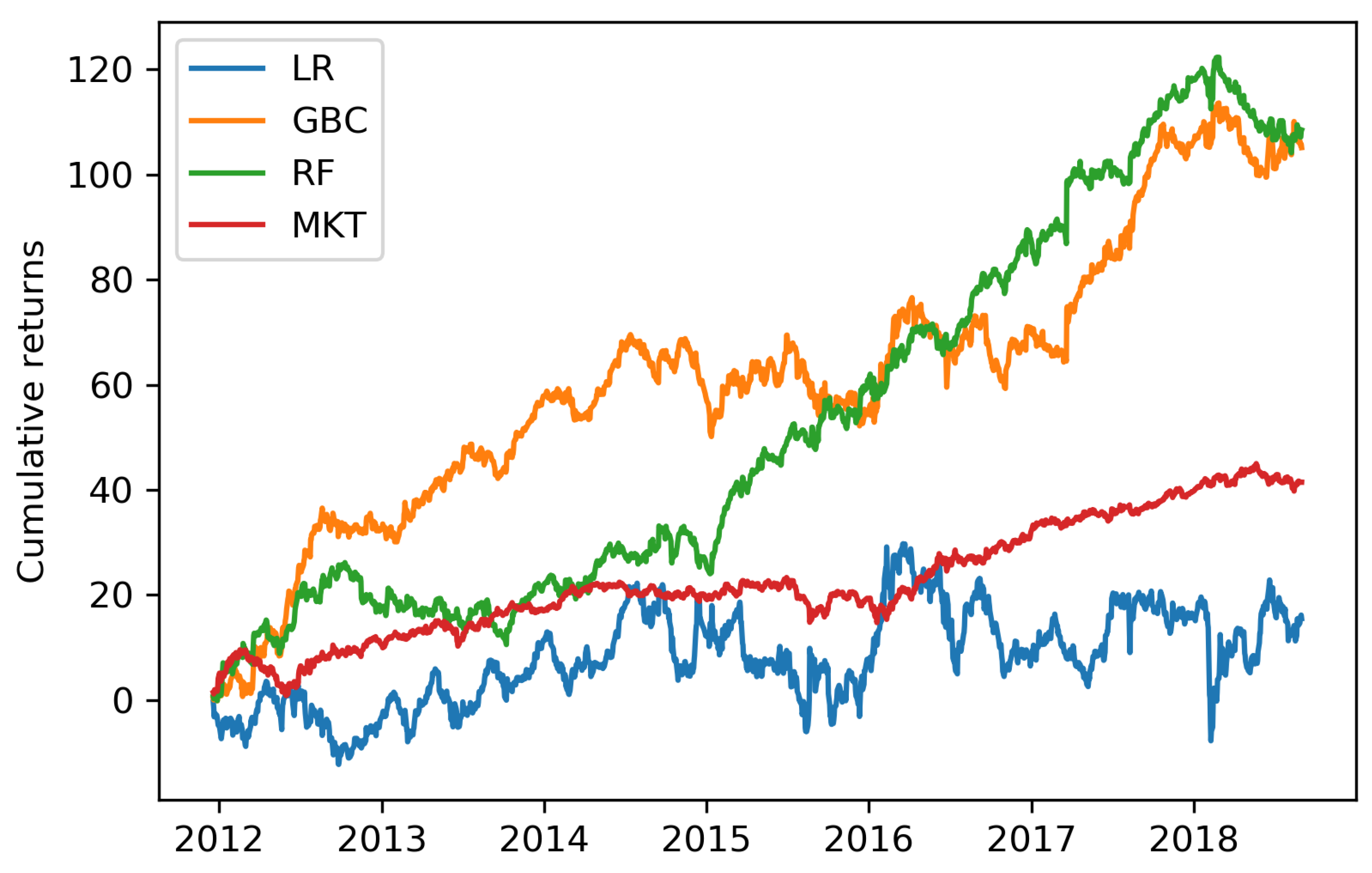
Cumulative returns: The above findings translate into cumulative returns as depicted in Figure 1. The MKT outperforms the LR by a delta of more than 25 percent by the end of the trading simulation. By contrast, trading based on the GBC and the RF compares favorably to the performance of the MKT. Thereby, the seven study periods can be divided into two parts. Between 2012 and 2015, the MKT accumulates returns similar to those of the RF and is clearly outperformed by the GBC. From 2015 onwards, both the MKT’s and the tree-based model’s profit accumulation follows an upward trend, however, that of the GBC and the RF is more pronounced. The improved performance of the tree-based models in the second half of the trading simulation may be due to the fact that the number of tradable futures increases from 73 in the first study period to 98 in the last study period. As such, our rules-based portfolio construction mechanism can choose from a greater futures universe in the later study periods. Because futures markets typically allow for large degrees of leverage (Ang et al. (2011) estimate a range of 10 to 50), the results present a lower boundary for the profit potential of our trading strategy.
Compared to the LR, the tree-based models lead to increased model complexity and computational costs. However, the tree-based trading strategies outperform those based on the LR by far. Consequentially, the benefits in terms of profit accumulation clearly outweigh the additional efforts when trading based on the RF and the GBC.
4.1.2. Feature Importance
Figure 2 depicts the relative feature importance for the LR, GBC and RF as an average over all study periods. The feature importance for the LR is calculated by multiplying the coefficients with the corresponding standard deviations. denotes the periodic return calculated over l periods, as defined in Equation (1). The most important variable is standardized to 100 for each model.
The tree-based models show a very similar pattern, as the returns of the first five days are among the ten most important features. As such, both models seem to heavily rely on the most recent price history when predicting the one-day ahead return. Features capturing long-term price movements are the second most important when analyzing the top ten, as both models include the features , and . Medium-term features ranging from to are less important when making predictions. Upon analyzing the feature importance for the LR, a similar but less pronounced pattern emerges. Among the top ten, five short-term, three long-term and two medium-term features are included.
Our results are in line with Krauss et al. (2017) and Fischer et al. (2019), who both find that short-term features exhibit the largest explanatory power in equity markets. The high importance of short-term features could be driven by short-term reversal effects, as discussed, for example, in Jegadeesh (1990); Lehmann (1990) and Lo and MacKinlay (2015). By incorporating this effect, the models seem to assume that futures falling sharply in the short term tend to rise during subsequent periods, and vice versa.
4.2. Varying Portfolio Size
In the baseline scenario, we open long/short positions for the top/flop three futures each day. In this subsection, we deviate from our baseline strategy and vary the number of traded futures. We analyze the model performance based on the top/flop one , top/flop two and top/flop five trading portfolios and contrast it to the baseline top/flop three scenario. As the LR does not generate statistically and economically significant results in the baseline scenario, it is omitted in the following analysis. The results are depicted in Table 2.
Daily return characteristics: Panel A of Table 2 reveals that the break-even transaction costs are largest for the top/flop one trading strategy (13.2 bp for the GBC and 13.1 bp for the RF) and gradually decrease with the number of traded futures. This is in line with Huck (2009) and Krauss et al. (2017), who find that increasing the number of traded equities leads to decreasing returns. When splitting realized break-even transaction costs into long and short positions, we find that long positions yield larger break-even transaction costs compared to short positions. Trading across all portfolio sizes and model combinations yields statistically significant break-even transaction costs, with t-statistics ranging from 2.3 to 3.2.
Daily risk characteristics: As illustrated in Panel B of Table 2, the maximum drawdown is lowest for the top/flop five trading strategy (−9.2 percent for the GBC and −10.7 percent for the RF) and increases with portfolio size. This ranking is reflected in the VaR, where the top/flop five trading strategy compares most favorably. As such, the decreasing break-even transaction costs are accompanied by lower risks when increasing the number of traded futures.
Annualized risk-return metrics: As shown in Panel C of Table 2, we find that annual returns are largest for the top/flop one trading strategy and decrease with the number of traded futures. Considering risk-adjusted ratios, most metrics remain at similar levels irrespective of the size of the traded portfolio. For example, the Sharpe ratio of the RF model remains close to 1.2, which can be explained by the fact that the decreasing break-even transaction costs are outweighed by a similarly fast decrease in volatility when expanding the number of traded futures.
4.3. Varying Holding Period
In this subsection, we return to our baseline top/flop three trading strategy and analyze model performance with respect to variations in the holding period h. Specifically, we increase the holding period to two and three days, respectively, and retrain the models for every configuration.
In the case of holding periods longer than one day, we open a new portfolio each day and fund it with of the overall investment capital. In the following analysis, we additionally compute daily mean returns next to break-even transaction costs, as they differ when expanding the holding period above one day. The former reveals the average return over all the portfolios active at time t, while the latter shows the transaction costs leading to a return of zero per full turn. As above, we restrict our analysis to the performance of the GBC and the RF. Table 3 depicts the results.
Break-even transaction cost: As illustrated in Panel A of Table 3, expanding the holding period from one to three days leads to larger break-even transaction costs for both the GBC (6.1 bp to 24.2 bp) and the RF (6.3 bp to 18.6 bp). Increases in break-even transaction costs when prolonging the holding period are to be expected, as the return volatility typically increases with the length of the holding period. Comparing the contributions from long and short trades, we find that the former consistently produces larger break-even transaction costs irrespective of the holding period.
Daily return characteristics: Considering mean returns (Panel B of Table 3), we find that no clear pattern emerges when expanding the holding period. When analyzing the daily returns of the strategy, several positive and negative effects are overlapping, which are very difficult to disentangle given the high degree of noise in financial time series. First, the quality of the signal usually decreases with longer holding periods, i.e., it is typically more difficult to predict longer than shorter time horizons. Second, longer holding periods allow for larger price fluctuations and higher returns, but also for higher risk—in particular due to the limited number of simultaneous positions in a portfolio. Third, in the case that the holding periods are longer than one day, we open a new portfolio each day and equally split the available investment capital across all the active portfolios. This partly decreases risk, as not all the active portfolios hold the same futures (i.e., the aggregate of the active portfolios is more diversified). When moving from two to three days, the observed increase in break-even transaction costs (from 7.8 bp to 24.2 bp for the GBC and from 10.4 bp to 18.6 bp for the RF) indicates that the above mentioned negative effects of the longer holding period are potentially overcome by the above mentioned positive effects (the increase in break-even transaction costs is much larger than from one to two days). Standard deviations decrease from 0.010 (GBC) and 0.008 (RF) in the case of a holding period of one day to 0.006 (GBC) and 0.005 (RF) when holding positions for three days.
Risk-return characteristics: Panel C in Table 3 reveals that the VaR is lowest at a holding period of three days for both models. Considering risk-return metrics, we find that the Sharpe ratio tends to increase with the holding period.
5. Conclusions
In this study, we successfully transfer a well-established statistical arbitrage trading strategy based on machine learning from equities to futures markets. After addressing peculiarities specific to futures trading, we train logistic regressions, random forests and gradient-boosting classifiers based on lagged returns of a defined trading universe comprised of 60 futures. With the trained models, we aim to predict the directional h-day-ahead development of each future and enter long/short positions for the top/flop-k predictions. Our trading strategy is based on a classification instead of a regression task, as the existing literature has shown that the former typically outperforms the latter in financial machine learning applications (see, e.g., Enke and Thawornwong 2005; Leung et al. 2000). Whether this also holds true in futures markets is subject to further research.
In a baseline scenario (, ), the machine learning models outperform the general market (i.e., an equally weighted buy-and-hold strategy for the constructed futures portfolios) by far, which poses a clear challenge to the semi-strong form of market efficiency (Fama 1970) in futures markets. Considering the implemented machine learning models, Fischer and Kraus (2018) demonstrate the superiority of statistical arbitrage strategies based on deep neural networks compared to tree-based algorithms when trading in equity markets. Whether this finding can be transferred to futures markets is another direction for further research.
Analyzing feature importance, we find that short-term patterns are utilized the most by the machine learning models when making out-of-sample predictions, suggesting a strong reliance on short-term reversal effects in the data. Because the machine learning models deployed in equity markets seem to rely on similar patterns, the two markets could allow for transfer learning, where models trained based on equity prices could generate profitable trading signals in futures markets, and vice versa. This is subject to further research.
Finally, we analyze the robustness of our findings by varying the number of traded futures k and the holding period h, respectively. Trading the top/flop one futures increases the model performance in terms of realized break-even transaction costs twofold compared to the baseline top/flop three trading strategy—a well documented finding in the financial machine learning literature (see, e.g., Huck 2009; Krauss et al. 2017). However, this comes at the cost of increased risk. Furthermore, we find that break-even transaction costs increase with the length of the holding period, accompanied by improved risk-return metrics.
Author Contributions
Conceptualization, F.W. and M.S.; data curation, F.W.; methodology, C.K. and T.G.F.; software, F.W. and M.S.; validation, F.W., M.S., C.K. and T.G.F.; visualization, F.W.; project administration, F.W. and M.S.; funding acquisition, F.W; writing—original draft preparation, F.W. and M.S.; writing—review and editing, C.K. and T.G.F. All authors have read and agreed to the published version of the manuscript.
Funding
This research received no external funding.
Acknowledgments
Thanks go to the anonymous reviewers for their valuable suggestions. Furthermore, we are grateful to the “FAU Open Access Publikationsfonds”, which has covered 75 percent of the publication fees.
Conflicts of Interest
The authors declare no conflict of interest.
Abbreviations
The following abbreviations are used in this manuscript:
| DTN | DTN IQFeed |
| VWAP | Volume-weighted average price |
| EST | Eastern Standard Time |
| LR | Logistic regression |
| RF | Random forest |
| GBC | Gradient-boosting classifier |
| MKT | General market |
| VaR | Value at risk |
References
- Ang, Andrew, Sergiy Gorovyy, and Gregory B. Van Inwegen. 2011. Hedge fund leverage. Journal of Financial Economics 102: 102–26. [Google Scholar] [CrossRef]
- Berkowitz, A. Stephen, E. Dennis Logue, and A. Eugene Noser. 1988. The total cost of transactions on the NYSE. The Journal of Finance 43: 97–112. [Google Scholar] [CrossRef]
- Breiman, Leo. 2001. Random forests. Machine Learning 45: 5–32. [Google Scholar] [CrossRef] [Green Version]
- Dare, Wale. 2017. Statistical Arbitrage in the U.S. Treasury Futures Market. Economics Working Paper Series; St. Gallen: University of St. Gallen, vol. 1716. [Google Scholar]
- Dixon, Matthew, Diego Klabjan, and Jin Bang. 2017. Classification-based financial market prediction using deep neural networks. Algorithmic Finance 6: 67–77. [Google Scholar] [CrossRef] [Green Version]
- Enke, David, and Suraphan Thawornwong. 2005. The use of data mining and neural networks for forecasting stock market returns. Expert Systems with Applications 29: 927–40. [Google Scholar] [CrossRef]
- Fama, Eugene F. 1970. Efficient capital markets: A review of theory and empirical work. The Journal of Finance 25: 383–417. [Google Scholar] [CrossRef]
- Fischer, Thomas, and Christopher Krauss. 2018. Deep learning with long short-term memory networks for financial market predictions. European Journal of Operational Research 270: 654–69. [Google Scholar] [CrossRef] [Green Version]
- Fischer, Thomas, Christopher Krauss, and Alexander Deinert. 2019. Statistical arbitrage in cryptocurrency markets. Journal of Risk and Financial Management 12: 31. [Google Scholar] [CrossRef] [Green Version]
- Focardi, Sergio, Frank Fabozzi, and Mitov Ivan. 2016. A new approach to statistical arbitrage: Strategies based on dynamic factor models of prices and their performance. Journal of Banking & Finance 65: 134–55. [Google Scholar]
- Girma, Paul Berhanu, and Albert S. Paulson. 1999. Risk arbitrage opportunities in petroleum futures spreads. Journal of Futures Markets 19: 931–55. [Google Scholar] [CrossRef]
- Harris, Charles R., K. Jarrod Millman, Stéfan J. van der Walt, Ralf Gommers, Pauli Virtanen, David Cournapeau, Eric Wieser, Julian Taylor, Sebastian Berg, Nathaniel J. Smith, and et al. 2020. Array programming with NumPy. Nature 585: 357–62. [Google Scholar] [CrossRef]
- Henrique, Bruno Miranda, Vinicius Amorim Sobreiro, and Herbert Kimura. 2019. Literature review: Machine learning techniques applied to financial market prediction. Expert Systems with Applications 124: 226–51. [Google Scholar] [CrossRef]
- Ho, Tin Kam. 1995. Random decision forests. Proceedings of 3rd International Conference on Document Analysis and Recognition 1: 278–282. [Google Scholar]
- Huck, Nicolas. 2009. Pairs selection and outranking: An application to the S&P 100 index. European Journal of Operational Research 196: 819–25. [Google Scholar]
- Huck, Nicolas. 2019. Large data sets and machine learning: Applications to statistical arbitrage. European Journal of Operational Research 278: 330–42. [Google Scholar] [CrossRef]
- iqfeed.net. 2019. DTN Prosper in a Dynamic World. Available online: https://www.dtn.com (accessed on 29 December 2020).
- Jegadeesh, Narasimhan. 1990. Evidence of predictable behavior of security returns. The Journal of Finance 45: 881–98. [Google Scholar] [CrossRef]
- Ke, Guolin, Qi Meng, Thomas Finley, Taifeng Wang, Wei Chen, Weidong Ma, Qiwei Ye, and Tie-Yan Liu. 2017. LightGBM: A highly efficient gradient boosting decision tree. Proceedings of the 31st International Conference on Neural Information Processing Systems 30: 3149–57. [Google Scholar]
- Kleinbaum, David, and Mitchel Klein. 2010. Logistic Regression: A Self-Learning Text. New York: Springer. [Google Scholar]
- Krauss, Christopher. 2017. Statistical arbitrage pairs trading strategies: Review and outlook. Journal of Economic Surveys 31: 513–45. [Google Scholar] [CrossRef]
- Krauss, Christopher, Xuan Anh Do, and Nicolas Huck. 2017. Deep neural networks, gradient-boosted trees, random forests: Statistical arbitrage on the S&P 500. European Journal of Operational Research 259: 689–702. [Google Scholar]
- Lehmann, Bruce N. 1990. Fads, martingales, and market efficiency. The Quarterly Journal of Economics 105: 1–28. [Google Scholar] [CrossRef]
- Leung, Mark T., Hazem Daouk, and An-Sing Chen. 2020. Forecasting stock indices: A comparison of classification and level estimation models. International Journal of Forecasting 16: 173–90. [Google Scholar] [CrossRef]
- Lo, Andrew W., and A. Craig MacKinlay. 2015. When are contrarian profits due to stock market overreaction? The Review of Financial Studies 3: 175–205. [Google Scholar] [CrossRef]
- Masteika, Saulius, Rutkauskas V. Aleksandras, and Janes Andrea Aleksandra. 2012. Continuous futures data series for back testing and technical analysis. Conference Proceedings, 3rd International Conference on Financial Theory and Engineering 29: 265–69. [Google Scholar]
- McKinney, Wes. 2010. Data structures for statistical computing in Python. Paper presented at the 9th Python in Science Conference, Austin, TX, USA, June 28–July 3; vol. 445, pp. 56–61. [Google Scholar]
- Nakajima, Tadahiro. 2019. Expectations for statistical arbitrage in energy futures markets. Journal of Risk and Financial Management 12: 14. [Google Scholar] [CrossRef] [Green Version]
- Pedregosa, Fabian, Gaël Varoquaux, Alexandre Gramfort, Vincent Michel, Bertrand Thirion, Olivier Grisel, Mathieu Blondel, Peter Prettenhofer, Ron Weiss, Vincent Dubourg, and et al. 2011. Scikit-learn: Machine learning in Python. Journal of Machine Learning Research 12: 2825–30. [Google Scholar]
- Python Software Foundation. 2018. Python 3.7.1 Documentation. Available online: https://www.python.org/downloads/release/python-371/ (accessed on 29 December 2019).
- Quantopian Inc. 2016. Empyrical: Common Financial Risk Metrics. Available online: https://github.com/quantopian/empyrical (accessed on 29 December 2019).
- Schnaubelt, Matthias. 2019. A comparison of machine learning model validation schemes for non-stationary time series data. FAU Discussion Papers in Economics 11. [Google Scholar]
- Schnaubelt, Matthias, Thomas Fischer, and Christopher Krauss. 2020. Separating the signal from the noise—Financial machine learning for Twitter. Journal of Economic Dynamics and Control 114: 103895. [Google Scholar] [CrossRef] [Green Version]
- Seabold, Skipper, and Josef Perktold. 2010. Statsmodels: Econometric and statistical modeling with Python. Paper presented at the 9th Python in Science Conference, Austin, TX, USA, June 28–July 3. [Google Scholar]
- Sezer, Omer Berat, Mehmet Ugur Gudelek, and Ahmet Murat Ozbayoglu. 2020. Financial time series forecasting with deep learning: A systematic literature review: 2005–2019. Applied Soft Computing 90: 106181. [Google Scholar] [CrossRef] [Green Version]
- Simon, David P. 1999. The soybean crush spread: Empirical evidence and trading strategies. Journal of Futures Markets 19: 271–89. [Google Scholar] [CrossRef]
- Stevens Analytics. 2019. Continuous Futures. Available online: https://www.quandl.com/databases/SCF/documentation (accessed on 29 December 2020).
- Takeuchi, Lawrence, and Yu-Ying Albert Lee. 2013. Applying Deep Learning to Enhance Momentum Trading Strategies in Stocks. Working Paper. Stanford: Stanford University. [Google Scholar]
- Vojtko, Radovan, and Matus Padysak. 2020. Continuous Futures Contracts Methodology for Backtesting. Available online: https://ssrn.com/abstract=3517736 or https://0-dx-doi-org.brum.beds.ac.uk/10.2139/ssrn.3517736 (accessed on 15 January 2021).
- Zuckerman, Gregory. 2019. The Man Who Solved the Market. London: Penguin Books Limited. [Google Scholar]
| 1 | |
| 2 | By not including the trading set, we only consider information that is available up to the time of predicting out of sample. |
Figure 1.
Cumulative returns for baseline strategy. Cumulative returns expressed in percentage terms for the top/flop three trading strategy for the logistic regression (LR), gradient-boosting classifier (GBC), random forest (RF) and general market (MKT) over the seven-period-long trading simulation with a holding period of one day .

Figure 2.
Feature importance. Average feature importance for the logistic regression (LR), gradient-boosting classifier (GBC) and random forest (RF). The most important feature is standardized to 100. Average feature importance is depicted for the top/flop three trading strategy and a holding period of one day .


Table 1.
Strategy performance of baseline scenario. Daily return characteristics (Panel A), daily risk characteristics (Panel B) and annualized risk-return metrics (Panel C) for the logistic regression (LR), gradient-boosting classifier (GBC), random forest (RF) and general market (MKT). Performance characteristics are illustrated for the top/flop three trading strategy and a holding period of one day . NW denotes Newey–West standard errors with one-lag correction. Daily value at risk (VaR) is calculated at the 95.0 percent confidence level.
| LR | GBC | RFC | MKT | ||
|---|---|---|---|---|---|
| A | Break-even transaction cost | 0.00009 | 0.00061 | 0.00063 | 0.00024 |
| Break-even transaction cost (long) | 0.00052 | 0.00109 | 0.00118 | - | |
| Break-even transaction cost (short) | −0.00015 | 0.00013 | 0.00007 | - | |
| t-Statistic (NW) | 0.30579 | 2.62765 | 3.11186 | 2.52548 | |
| Minimum | −0.12808 | −0.04298 | −0.04027 | −0.02482 | |
| Quartile 1 | −0.00590 | −0.00459 | −0.00330 | −0.00214 | |
| Median | 0.00028 | 0.00029 | 0.00016 | 0.00033 | |
| Quartile 3 | 0.00590 | 0.00524 | 0.00421 | 0.00252 | |
| Maximum | 0.09844 | 0.09933 | 0.11678 | 0.01877 | |
| Standard deviation | 0.01224 | 0.00965 | 0.00841 | 0.00396 | |
| Skewness | −0.32935 | 0.87212 | 2.09778 | −0.03325 | |
| Kurtosis | 11.56410 | 9.18384 | 25.57640 | 2.55999 | |
| Share > 0 | 0.50874 | 0.51573 | 0.51573 | 0.53555 | |
| B | VaR | −0.02439 | −0.01871 | −0.01620 | −0.00768 |
| Maximum drawdown | −0.34114 | −0.18039 | −0.16953 | −0.08429 | |
| C | Annualized return | 0.00383 | 0.15331 | 0.16232 | 0.06067 |
| Calmar ratio | 0.01124 | 0.84986 | 0.95750 | 0.71971 | |
| Sharpe ratio | 0.11715 | 1.00666 | 1.19216 | 0.96752 | |
| Sortino ratio | 0.16416 | 1.58896 | 2.00973 | 1.43528 |
Table 2.
Strategy performance for variations in the number of traded futures. Daily return characteristics (Panel A), daily risk characteristics (Panel B) and annualized risk-return metrics (Panel C) for the gradient-boosting classifier (GBC) and random forest (RF). Performance characteristics are illustrated for the top/flop one , top/flop two , top/flop three and top/flop five trading strategies and a holding period of one day . NW denotes Newey–West standard errors with one-lag correction. VaR is calculated at the 95.0 percent confidence level.
| Top/Flop One | Top/Flop Two | Top/Flop Three | Top/Flop Five | ||||||
|---|---|---|---|---|---|---|---|---|---|
| GBC | RF | GBC | RF | GBC | RF | GBC | RF | ||
| A | Break-even transaction cost | 0.00132 | 0.00131 | 0.00090 | 0.00083 | 0.00061 | 0.00063 | 0.00037 | 0.00046 |
| Break-even transaction cost (long) | 0.00180 | 0.00192 | 0.00153 | 0.00156 | 0.00109 | 0.00118 | 0.00076 | 0.00092 | |
| Break-even transaction cost (short) | 0.00085 | 0.00069 | 0.00027 | 0.00010 | 0.00013 | 0.00007 | −0.00001 | 0.00000 | |
| t-Statistic (NW) | 2.76110 | 3.11080 | 2.93075 | 3.15662 | 2.62764 | 3.11186 | 2.25589 | 3.07501 | |
| Minimum | −0.10135 | −0.10135 | −0.05926 | −0.05835 | −0.04299 | −0.04027 | −0.03273 | −0.02740 | |
| Quartile 1 | −0.00740 | −0.00496 | −0.00543 | −0.00383 | 0.00460 | −0.00330 | −0.00344 | −0.00271 | |
| Median | 0.00047 | 0.00045 | 0.00028 | 0.00034 | 0.00029 | 0.00016 | 0.00024 | 0.00014 | |
| Quartile 3 | 0.00867 | 0.00622 | 0.00615 | 0.00496 | 0.00524 | 0.00421 | 0.00378 | 0.00335 | |
| Maximum | 0.27963 | 0.35127 | 0.14794 | 0.17182 | 0.09933 | 0.11678 | 0.05810 | 0.07125 | |
| Standard deviation | 0.01994 | 0.01738 | 0.01280 | 0.01095 | 0.00965 | 0.00841 | 0.00690 | 0.00620 | |
| Skewness | 2.35936 | 5.99524 | 1.20400 | 2.89764 | 0.87212 | 2.09778 | 0.44085 | 1.33217 | |
| Kurtosis | 28.13396 | 106.51918 | 13.53247 | 40.63920 | 9.18384 | 25.57640 | 5.58418 | 12.04839 | |
| Share > 0 | 0.51457 | 0.52448 | 0.51457 | 0.52098 | 0.51573 | 0.51573 | 0.51981 | 0.51807 | |
| B | VaR | −0.03856 | −0.03348 | −0.02471 | −0.02109 | −0.01870 | −0.01620 | −0.01344 | −0.01195 |
| Maximum drawdown | −0.36443 | −0.29841 | −0.22777 | −0.21107 | −0.18039 | −0.16953 | −0.16371 | −0.10751 | |
| C | Annualized return | 0.33113 | 0.34041 | 0.23095 | 0.21592 | 0.15330 | 0.16232 | 0.09286 | 0.11760 |
| Calmar ratio | 0.90862 | 1.14075 | 1.01394 | 1.02302 | 0.84985 | 0.95749 | 0.56721 | 1.09389 | |
| Sharpe ratio | 1.05778 | 1.19175 | 1.12278 | 1.20931 | 1.00665 | 1.19216 | 0.86424 | 1.17804 | |
| Sortino ratio | 1.81288 | 2.32253 | 1.81317 | 2.09544 | 1.58895 | 2.00973 | 1.31664 | 1.92731 | |
Table 3.
Strategy performance for varying holding periods. Break-even transaction costs (Panel A), daily return characteristics (Panel B) and risk-return metrics (Panel C) for the gradient-boosting classifier (GBC) and random forest (RF). Performance characteristics are illustrated for the top/flop three trading strategy and holding periods of one , two and three days. NW denotes Newey–West standard errors with one-lag correction. VaR is calculated at the 95.0 percent confidence level.
| One Day | Two Days | Three Days | |||||
|---|---|---|---|---|---|---|---|
| GBC | RF | GBC | RF | GBC | RF | ||
| A | Break-even transaction cost | 0.00061 | 0.00063 | 0.00078 | 0.00104 | 0.00242 | 0.00186 |
| Break-even transaction cost (long) | 0.00109 | 0.00156 | 0.00157 | 0.00160 | 0.00313 | 0.00237 | |
| Break-even transaction cost (short) | 0.00013 | 0.00010 | 0.00000 | 0.00050 | 0.00172 | 0.00134 | |
| t-Statistic (NW) | 2.62764 | 3.11186 | 2.11017 | 3.51750 | 5.49028 | 5.02821 | |
| B | Mean return | 0.00061 | 0.00063 | 0.00038 | 0.00052 | 0.00080 | 0.00062 |
| Minimum | −0.04299 | −0.04027 | −0.08987 | −0.06418 | −0.04005 | −0.03910 | |
| Quartile 1 | −0.00460 | −0.00330 | −0.00332 | −0.00248 | −0.00252 | −0.00212 | |
| Median | 0.00029 | 0.00016 | 0.00034 | 0.00026 | 0.00043 | 0.00030 | |
| Quartile 3 | 0.00524 | 0.00421 | 0.00398 | 0.00330 | 0.00373 | 0.00283 | |
| Maximum | 0.09933 | 0.11678 | 0.06045 | 0.05670 | 0.04081 | 0.04362 | |
| Standard deviation | 0.00965 | 0.00841 | 0.00761 | 0.00615 | 0.00609 | 0.00511 | |
| Skewness | 0.87212 | 2.09778 | −1.08371 | −0.13586 | 0.69039 | 0.99260 | |
| Kurtosis | 9.18384 | 25.57640 | 18.22652 | 14.86417 | 6.46430 | 12.39674 | |
| Share > 0 | 0.51573 | 0.51573 | 0.52273 | 0.52389 | 0.53438 | 0.53846 | |
| C | Annualized return | 0.15330 | 0.16232 | 0.09462 | 0.13518 | 0.21999 | 0.16559 |
| VaR | −0.01870 | −0.01620 | −0.01485 | −0.01178 | −0.01138 | −0.00961 | |
| Maximum drawdown | −0.18039 | −0.16953 | −0.26101 | −0.12467 | −0.11512 | −0.11325 | |
| Calmar ratio | 0.84985 | 0.95749 | 0.36252 | 1.08426 | 1.91081 | 1.46219 | |
| Sharpe ratio | 1.00665 | 1.19216 | 0.80841 | 1.34756 | 2.10334 | 1.92632 | |
| Sortino ratio | 1.58895 | 2.00973 | 1.14286 | 2.06169 | 3.56316 | 3.28521 | |
Publisher’s Note: MDPI stays neutral with regard to jurisdictional claims in published maps and institutional affiliations. |
© 2021 by the authors. Licensee MDPI, Basel, Switzerland. This article is an open access article distributed under the terms and conditions of the Creative Commons Attribution (CC BY) license (http://creativecommons.org/licenses/by/4.0/).
Share and Cite
MDPI and ACS Style
Waldow, F.; Schnaubelt, M.; Krauss, C.; Fischer, T.G. Machine Learning in Futures Markets. J. Risk Financial Manag. 2021, 14, 119. https://0-doi-org.brum.beds.ac.uk/10.3390/jrfm14030119
AMA Style
Waldow F, Schnaubelt M, Krauss C, Fischer TG. Machine Learning in Futures Markets. Journal of Risk and Financial Management. 2021; 14(3):119. https://0-doi-org.brum.beds.ac.uk/10.3390/jrfm14030119
Chicago/Turabian StyleWaldow, Fabian, Matthias Schnaubelt, Christopher Krauss, and Thomas Günter Fischer. 2021. "Machine Learning in Futures Markets" Journal of Risk and Financial Management 14, no. 3: 119. https://0-doi-org.brum.beds.ac.uk/10.3390/jrfm14030119