
Month-End Regularities in the Overnight Bank Funding Markets

1
Department of Business Administration and Economics, Saint Mary’s College, Notre Dame, IN 46556, USA
2
Area of Finance, Rawls College of Business, Texas Tech University, Lubbock, TX 79409, USA
*
Author to whom correspondence should be addressed.
J. Risk Financial Manag. 2021, 14(5), 204; https://0-doi-org.brum.beds.ac.uk/10.3390/jrfm14050204
Submission received: 22 March 2021
/
Revised: 22 April 2021
/
Accepted: 27 April 2021
/
Published: 3 May 2021
(This article belongs to the Special Issue Financial Markets in Times of Crisis)
Abstract
:The money market rates in the United States exhibit various calendar patterns that are grounded in institutional and regulatory factors. In this paper, we document a new regularity in the overnight fed funds market. Specifically, we identify patterns of decreased volatility along with consistent and significant month-end rate drops in the fed fund rates. Our findings suggest that short-term liquidity requirements of the Basel III reforms are, in part, responsible for the regularity in fed funds.
JEL Classification:
G10; G21; G23; G281. Introduction
Rozeff and Kinney (1976) start a large body of academic literature on empirical calendar-based regularities. Three primary explanations of the empirical regularities have been offered: (1) tax loss selling (Branch 1977; Roll 1983), window dressing (Haugen and Lakonishok 1987; Ritter 1988), and preferred habitats (Ogden 1987, 1990).
Empirical calendar-based regularities extend into the money markets. Park and Reinganum (1986) find a month-end pattern in treasury bills, which Ogden (1987) suggests is consistent with a preferred habitat. Griffiths and Winters (1997) find a year-end regularity in term government general collateral repos and Griffiths and Winters (2005) find year-end regularities in one-month private-issue money market securities. All the year-end regularities found in Griffiths and Winters (1997, 2005) are consistent with a preferred habitat for liquidity.
Regularities also appear in overnight federal (fed) funds, but the fed funds regularities are not calendar based as in the term money markets. The fed funds regularities follow directly from the Federal Reserve regulations for maintenance of reserves. Spindt and Hoffmeister (1988) find that daily fed funds rate volatility is highest on the last day (settlement Wednesdays) of the two-week reserve maintenance period. Extending Spindt and Hoffmeister (1988), Griffiths and Winters (1995) find rate change regularities across the reserve maintenance period with fed funds rates declining on Fridays and increasing every second Wednesday (settlement Wednesday). However, Kotomin and Winters (2007) document the dissipation of the settlement Wednesday effect in the federal funds market post July 1998, due to Federal Reserve’s regulatory change from contemporaneous to lag reserve requirements. With the understanding that previous regularities in fed funds come from regulations and with these studies as the backdrop, in this paper, we document a new regularity in the overnight fed funds markets.
Specifically, we identify a pattern of consistent rate drops on the last trading day of the month in fed funds that is accompanied with decreased daily volatility across all other trading days. The month-end rate drops occur every month from 31 December 2014 through 31 January 2018 (end of sample) and are economically significant with an average decline of 8.3 basis points. This regularity does not align with reserve maintenance rules, but, since fed funds are bank reserve deposits, this regularity may relate to banking regulations.
The appearance of the new regularity in fed funds aligns with the implementation of the Basel III liquidity coverage ratio (LCR) requirements, which begins in January 2015. Fed funds are a component in the monthly calculation of a bank’s LCR and the fed funds rate drop that we find is consistent with the actions a bank would take to improve their LCR. In other words, the fed funds rate drop is consistent with banks window dressing to improve their LCRs. Window dressing LCRs explains why the regularities in fed funds begin on 31 December 2014.
We note that Basel III also includes a new leverage ratio for banks. There is a body of literature on the leverage ratio and its impact on the fed funds market. The leverage ratio has quarterly reporting and the literature shows an associated quarterly regularity that begins in January 2013, which is two years before the implementation of the LCR. This literature also shows the absence of the monthly regularity before 31 December 2014.
2. Background
To properly position our findings, we provide a brief review of academic literature on the regularities in various money market rates. We follow the general discussion with a detailed discussion on fed funds.
2.1. Early Work
Gibbons and Hess (1981) investigate day of week patterns in various classes of asset returns. Their evidence from treasury bills suggests a below average return on Mondays with an above average return on Wednesdays. Park and Reinganum (1986) identify a price pattern on Treasury bills maturing at the turn of calendar months and at the turn of the year. The evidence presented by the authors suggests that the last T-bill to mature in a month trades at a lower yield (higher price) than surrounding T-bills. However, the authors were unable to explain this regularity. Ogden (1987) suggests that the findings of Park and Reinganum (1986) are consistent with a year-end preferred habitat for liquidity.
2.2. Preferred Habitat vs. Window Dressing
Musto (1997) argues that the year-end effect observed in the commercial paper market is consistent with the window dressing hypothesis. Commercial paper sells at an extra discount if it is maturing in the next calendar year, while T-bills do not share this pattern. Musto argues that this pattern is inconsistent with tax loss selling but is consistent with the window dressing hypothesis, whereby “intermediaries choose portfolios for disclosure dates, which underrepresent the riskiness of portfolios held on non-disclosure dates.” Musto’s analysis is based on the comparison of average rates over the last week of the year to the average rates over the first week of the next year. Using daily rate changes instead of weekly averages, Griffiths and Winters (1997, 2005) find a year-end effect in various money market instruments (including commercial paper). Griffiths and Winters (2005) show that the year-end pattern is consistent with a preferred habitat for liquidity hypothesis (Modigliani and Sutch 1966; Ogden 1987). Their empirical analysis indicates that the timing of year-end rate changes is inconsistent with other possible explanations, such as the window dressing hypothesis.
Allen and Saunders (1992) identify a quarter-end window dressing phenomenon in banks. Each quarter, banks have to report their balance sheet data to regulators (and ultimately investors), which provides banks with incentives to window dress. The authors suggest that money market instruments (federal funds, repos, cd, and Eurodollar deposits) act as vehicles for the upward window dressing from the liabilities side, while domestic loans, federal funds and repos sales are the asset side vehicles. Kotomin and Winters (2006) re-visit quarter-end bank window dressing from Allen and Saunders (1992). Kotomin and Winters (2006) provide evidence of an increase in (daily) fed funds rates at quarter-ends, but a decrease at year-ends. The authors argue that a year-end decrease in daily fed funds rate is not consistent with year-end window dressing.
A year-end effect attributable to the preferred habitat for liquidity is also observed in the London Interbank Offer Rate (LIBOR) market as well as its derivatives (Neely and Winters 2006; Kotomin et al. 2008; Kotomin 2011). Kotomin (2013) shows that the year-end pattern in various money market instruments was not present during the financial crisis of 2008–2009. Baig and Winters (2018) show that the year-end pattern attributable to the preferred habitat for liquidity in money markets reappeared after the financial crisis in government general collateral repo rates. In other words, money market participants seem to manage their year-end cash even in the post-crisis zero interest rate environment.
2.3. Federal Funds
Federal fund rates exhibit regularities. However, the systematic patterns in fed funds are different from other classes of money market instruments. This is due to rules and regulations for bank reserves and reserve maintenance. Eisemann and Timme (1984) investigate the intraweek seasonality in the fed fund rates. They argue that the seasonality corresponds to the reserve requirements, which induces banks to rely on the fed funds market to adjust their reserves. Griffiths and Winters (1995) show that reserve requirements result in predictable rate changes with rates declining on Fridays and increasing on settlement Wednesdays. Taken together, these studies show that fed funds rate changes have historically been known to exhibit calendar patterns.
Spindt and Hoffmeister (1988) model the “micromechanics” of the federal funds market and predict changes in the daily variance of rate changes at reserve maintenance pressure points. The empirical evidence shows that the variances of federal fund rates rise across the reserve maintenance period with the highest variance on settlement Wednesdays. Kopecky and Tucker (1993) point out that the variance of the daily federal funds rate is determined by the interaction of banks and the Federal Reserve, which is evident by the increased (about eight times) variance on settlement days, when compared to the non-settlement days. Griffiths and Winters (1995) suggest that the inter and intra period regulatory and accounting conventions strongly incentivize the institutions to borrow and lend in the federal funds market at predictable points (during the ten-trading day reserve maintenance period). Their analysis demonstrates that the regulatory requirements of the Fed cause non-constant daily and intraday volatility. Clouse and Elmendorf (1997) demonstrate that an increase in volatility of the fed funds rate can be explained by the low required reserve balances. However, the relation is nonlinear and continues to hold after controlling for changes in bank behavior across time. Similarly, Furfine (2000) identifies that empirical regularities in the volatility and level of daily fed funds rates correspond to the regularities in interbank payment flows/activity. Finally, Cyree and Winters (2001) find a reverse-J pattern in the intra-day volatility of federal funds, due to trading stoppages.
To the extent that the regularities in the federal funds market exist because of regulatory reasons, changes in the regulatory and accounting conventions should directly impact these patterns. Kotomin and Winters (2007) provide evidence of the dissipation of the settlement Wednesday effect in the federal funds market post July 1998. The authors argue that the Federal Reserve’s regulatory change from contemporaneous to lag reserve requirements (CRR to LRR) made it easier for banks to settle their reserve accounts. In essence, switching to the LRR regime reduced the demand for reserves on the settlement Wednesdays, which in turn reduced the settlement Wednesday effect and smoothed the effective federal funds rates in both level and volatility.
The fed funds market has had observable regularities in rate changes and volatility for decades. The regularities are a direct result of the rules and regulations of bank reserves and reserve maintenance. As the rules have changed over time to make reserve management simpler for banks the size of the regularities has declined. Our study demonstrates that following the financial crisis the old regularities have disappeared with a new and very different regularity appearing. We explore this new regularity in detail and offer a potential explanation.
2.4. Rates on Reserves
Milton (1960) argues in favor of the payment of market interest rates on bank reserves held at the Federal Reserve to improve the effectiveness of the monetary policy. A stream of academic literature that favored this proposition followed. Goodfriend (2002) suggests that interest on reserves not only strengthens and provides greater flexibility to the existing monetary policy tools available to the Fed but also provides a new tool in the form of the controllable payment of interest on reserves.
Under the Financial Services Regulatory Relief Act of 2006, the US Congress authorized the Federal Reserve to pay interest on reserves of depositary institutions starting in October 2011. However, in the midst of the financial crisis, on 18 December 2008, Federal Reserve decided to start paying 25 basis points on the reserves under the Emergency Economic Stabilization Act of 2008. The decision of Federal Reserve to pay interest on reserves should, in theory, establish a floor for the federal funds market, otherwise there could be arbitrage opportunities (Bernanke 2009). Griffiths et al. (2014) however suggest that the effective federal funds rate has always stayed below this “floor”. The authors argue that this apparent anomaly is not due to market inefficiency but exists essentially because of the inclusion of GSE overnight loans in the calculation of the effective federal funds rates, which is contrary to the traditional definition. GSEs are willing to accept lower rates on loans because their accounts at the Federal Reserve are prohibited for earning interest. The anomaly is also in part due to the costs accompanying “Federal Deposit Insurance Corporation (FDIC) assessment on the liabilities of depository institutions and capital charges, and the willingness of GSEs to lend to depository institutions”. None of these patterns or their underlying regulatory or institutional reasons, however, explain the new month-end regularity in fed funds.
3. Data
The daily data on effective federal funds rates (EFFR) used in this study is obtained from the Federal Reserve Economic Data (FRED) at the Federal Reserve Bank of St. Louis. The sample covers the period from the first trading day of January 2011 to the last trading day of January 2018. We begin the sample in January 2011 to exclude the financial crisis from our analysis. We choose to end our sample in January 2018 because in February 2018 the open market policy of the Federal Reserve experienced a structural change (Figure 1).
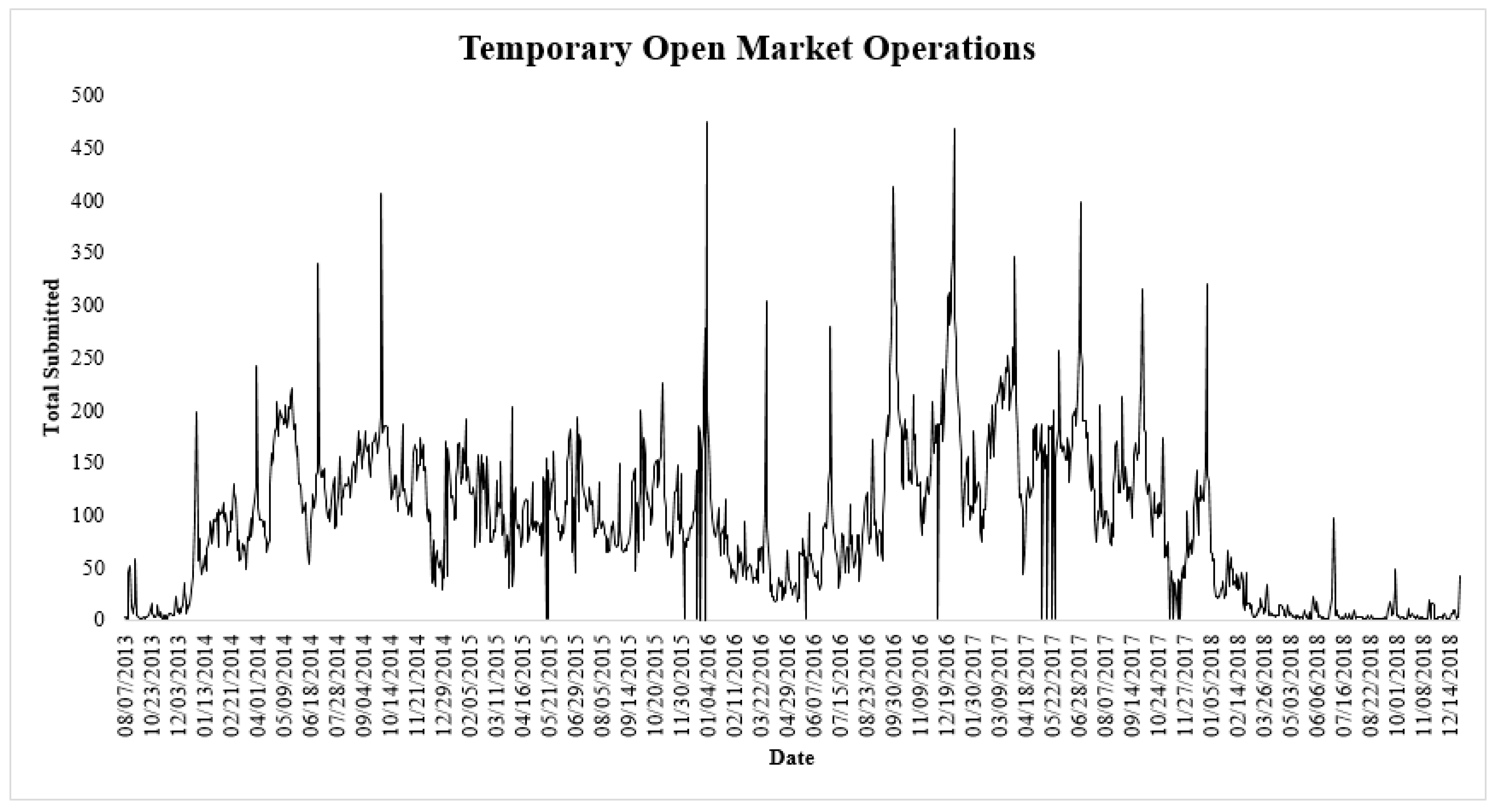
Money markets are for trading liquidity. The fed funds market is for banks to trade liquidity. The FOMC open market desk conducts open market operations to alter liquidity. The open market desk conducts temporary open market operations in terms from overnight to a few weeks. Figure 1 plots the daily dollar value (in $billion) of temporary open market operations across our sample. The data is available at: “https://apps.newyorkfed.org/markets/autorates/tomo-search-page (Last Accessed: 10 May 2019)”. Across our sample, 96.91% of temporary open market operations are overnight or across a weekend. Term temporary open market operations are the other 3.09% of the total with two-day operations at 1.91% and five to 28-day operations covering the other 1.18%. This plot provides several important insights. First, open market operations are small dollar prior to December 2013 where that plot shows a large spike up on 31 December 2013. Additionally, there are only 21 open market operations in 2011 and 2012 and all are less than $5 billion per day. Second, from December 2013 through January 2018, open market operations are large with the average at about $115 billion per day. Third, in March of 2018, open market operation returned to less than $5 billion per day. Finally, we plot the dollar value of temporary open market operations. Under temporary operations, the open market desk does repos to increase liquidity and reverse repos to decrease liquidity. For our sample, reverse repos are 98.7% of the total number temporary open market operations, which means that our sample period is under a policy regime of reducing liquidity. Reverse repos are 99.79% of the dollar value of temporary open market operations across our sample.
As noted in the introduction, the fed funds regularity starts on 31 December 2014, so it begins during the period of substantial temporary open market operations in reverse repos. We choose to end our sample on 31 December 2018, so our analysis of the regularity is conducted under one liquidity regime. The fed funds data from 2011 through 2014 provide a reference to benchmark the new regularity.
Table 1 presents the summary statistics of the sample. The table reports: number of observations, mean, median, standard deviation, 25th percentile and the 75th percentile of the rates, and changes in rates. Panel A of Table 1 provides statistics for the entire sample. The average effective federal funds rate in our full sample is 29.5 basis points (bps). We divide our sample into two sub-periods. The first sub-period covers the period of January 2011 through December 2014, while the second sub-period covers the period of January 2015 through January 2018.
Panel B of Table 1 provides statistics on the early sub-period (January 2011 through December 2014). The early sub-period is completely contained within one Federal Reserve interest rate regime, which is frequently referred to as the 0% rate regime. This regime spanned from 16 December 2008 through 17 December 2015, where the Fed targeted interest rates within a range on 0 to 25 basis points. The average fed funds rate is 11.0 bps.
Panel C of Table 1 reports statistics for our second sub-period (January 2015 through January 2018). This sub-period starts in the last year of the 0% rate regime, but the remainder of the sub-period is characterized by increasing policy target rates. In our second sub-period, the average fed funds rate is 53.5 bps.
4. Empirical Results
This study examines a new regularity in the overnight fed funds market. Our results section focuses exclusively on the empirical analysis of the regularity without any attempt to explain it. We present a possible explanation for the regularity in the discussion section that follows our empirical results.
Our empirical analysis focuses on descriptive statistics and economic significance. We feel that our approach is the best way to present our findings. We also feel our approach is appropriate because overnight money markets are low in default risk and do not include a term component. The reader will find footnotes discussing regressions where appropriate.
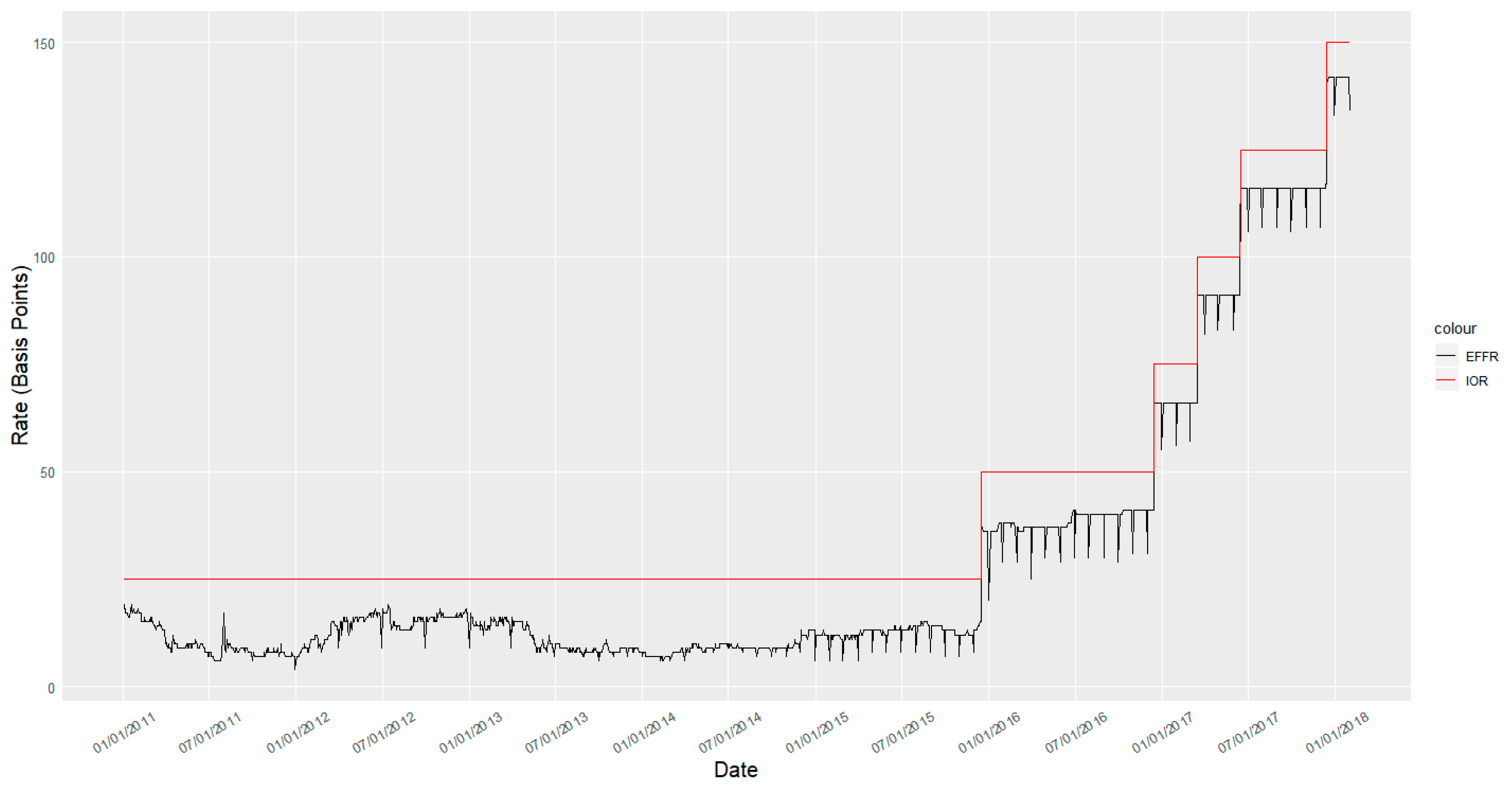
Figure 2 presents a time series plot of the daily effective federal funds rate and the interest rates on reserves (IOR) for the entire sample period (3 January 2011 to 31 January 2018). The plot has three distinctive features. First, we observe a consistent month-end rate drop starting from the last trading day of December 2014. Second, we observe almost no noise/variance in the daily rates following 1 January 2015. These results suggest an event at the end of 2014 that has affected the daily patterns of overnight fed funds rates. The month-end rate drop pattern appears to be economically weak during the first 12 months of its appearance (i.e., during 2015) and appears to become a lot more economically significant starting 2016. Third, the fed funds rate is below the IOR across our entire sample consistent with the findings in Griffiths et al. (2014).
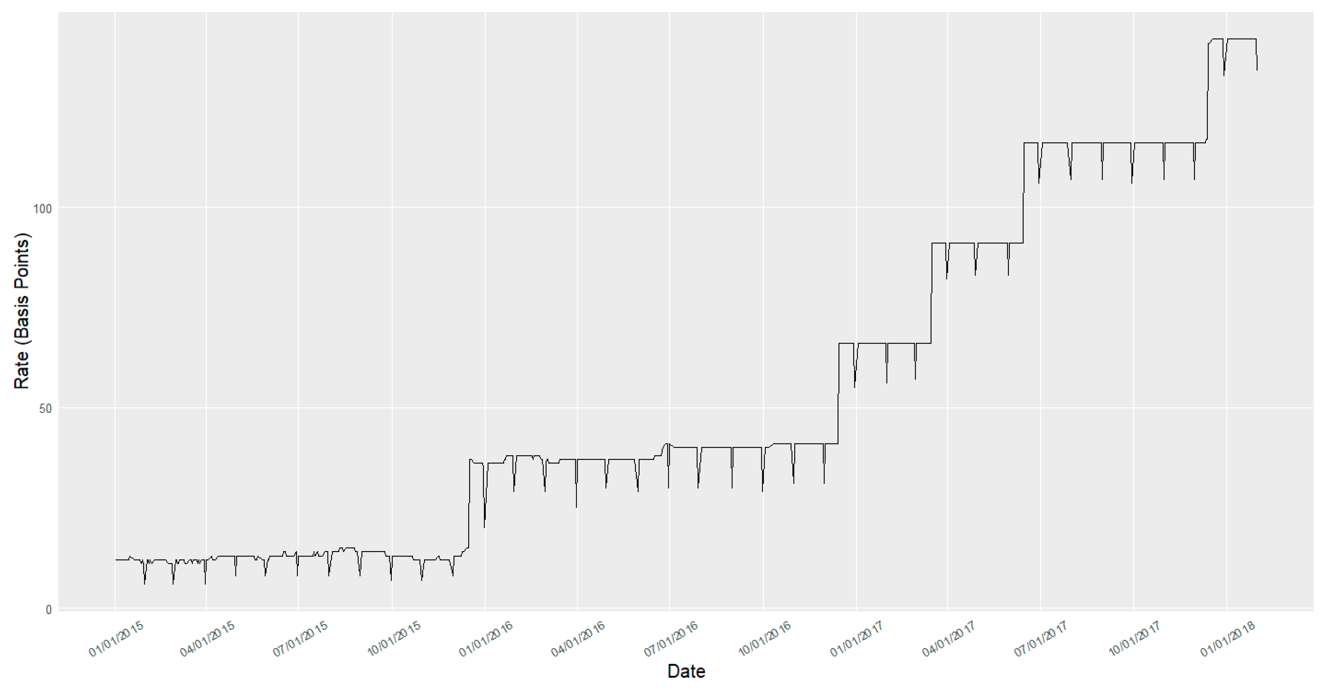
To provide a closer look the new pattern we break Figure 2 into two plots (Figure 3 and Figure 4) separated at the turn of the year from 2014 to 2015. Figure 3 shows that the fed funds rates are noisy during the 2011 through 2014 period and there appears to be no consistent pattern of month-end rate drops during this period. On the other hand, Figure 4 shows that beginning in 2015 daily fed funds rates are relatively constant throughout all trading days (recall, the steps up in rates are from policy target rate increases) except for the last trading day of every month, where we observe a substantial rate drop. Clearly, something changed and a new regularity/anomaly appeared in overnight fed funds rates. Equally clear is that the new regularity is not related to the settlement Wednesday effect in rates (Griffiths and Winters 1995) or variance (Spindt and Hoffmeister 1988).
This month-end rate drop pattern is unusual for the money market instruments. The only other identified month-end effect in money markets that we are aware of is by Park and Reinganum (1986) in T-bills and it is not isolated on the last trading day of the month. They observe that last T-bill to mature in a month trades at a yield lower than the surrounding T-bills. T-bills are discount instruments so lower yields come from higher prices. Ogden (1987) suggests that the pattern is consistent with a preferred habitat from the investors buying specific (month-end) T-bills. Such a case cannot be made for our month-end effect in federal funds. Fed funds are not discount instruments so lower rates are not consistent with preferring month-end fed funds.
We note that Figure 2 shows that IOR stays above the fed funds rate throughout the sample period. Another feature of the IOR plot is that rates are constant except for the jumps that correspond with the target rate changes. This is because IOR is a policy rate (not a market rate). On the other hand, fed funds is a market rate, so a volatile time series is expected. However, with the beginning of the regularity fed funds rates show little daily volatility except for the month-end rate drops and the daily volatility appears to decrease across time.
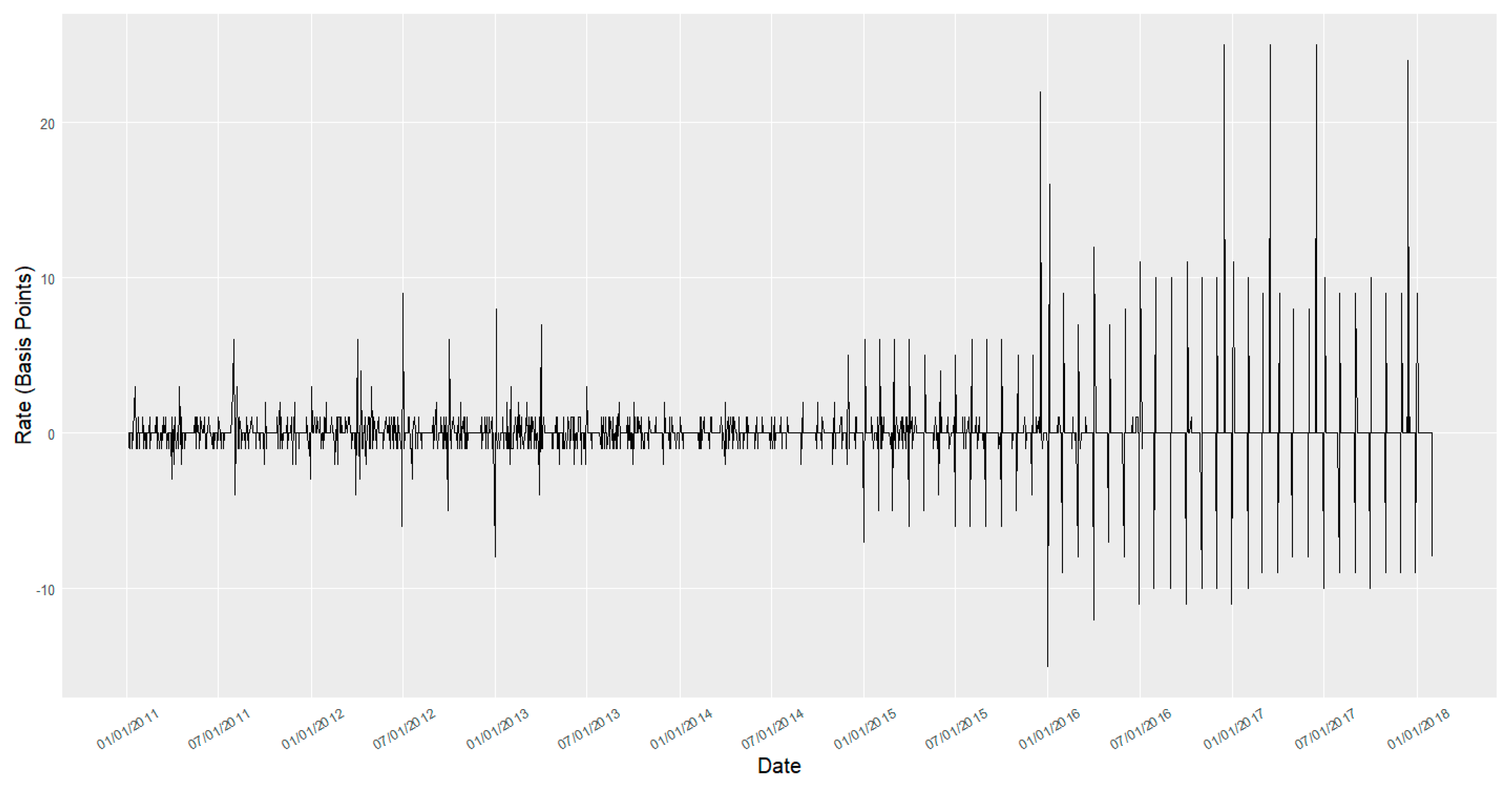
To provide a closer look at daily volatility, Figure 5 plots the time series of the Δ in effective fed funds rates for the entire sample period. We calculate the Δ effective fed funds rates as the daily first difference (EFFRt–EFFRt−1). Figure 5 shows that the consistent month-end rate drops are concentrated in our second sub-period (post 31 December 2014). The month-end rate drops are generally in a range of 5 to 10 bps, which is economically significant in money markets (see, Stigum and Crescenzi 2007). Additionally, the first sub-period is marked by significant daily changes of rates while the second sub-period shows decreasing daily volatility between the month-end rate drops.
These graphs present an overall picture of month-end rate drops in the second sub-period. Nevertheless, an argument could be made that the first sub-period could also contain month-end drops that are difficult to observe in the plots because they are hidden by daily noise/variance. To address this question and further motivate our argument of a consistent month-end effect in the second sub-period we compute the frequencies of month-end drops throughout the sample period. We identify the last trading day of each month throughout our sample period and record rate drops, rate hikes, and no change in rates relative to the previous trading day. Table 2 reports the results from this frequency analysis.
Table 2 Panel A summarizes the entire sample period. There are a total of 85 month-ends across our entire sample. Month-end rate drops occur in 64 out of the 85 months, there are rate hikes for 10 month-ends and 11 month-ends have no changes of rates. Note, there are 85 calendar month-ends across our sample. Accordingly, we have data in fed funds for every month-end in our sample. Table 2 Panel B reports the first sub-period. All 10 rate hikes and 11 constant rates from Panel A are in this sub-period. There are 27 month-end rate drops out of a total of 48 month-end observations from this period. Table 2 Panel C reports results for the second sub-period. There are no rate hikes or constant rates at month-ends during this period. Every single month-end (37 months out of a total of 37 month-end observations) is a rate drop.
The results reported in Table 2 confirm that there is a persistent month-end rate drop in effective fed funds rates in our second sub-period (January 2015 through January 2018).
Having identified a persistent month-end rate drop the next question is: are these rate drops statistically and/or economically significant? Stigum and Crescenzi (2007) state that a rate differential of 5 to 10 basis points is significant enough to induce arbitrage in the money markets, which provides an economic benchmark for our analysis. To investigate the magnitude and significance of the month-end effects we use daily ΔEFFR and calculate average month-end rate changes and average daily rates changes for all other market open days. We use means difference tests to compare the averages. In our unreported tests, we run a series of OLS regression of daily ΔEFFR on the month-end dummy and control for various factors in various different specifications. Our set of control variables include a dummy variable for policy rate changes, level and daily changes in the overnight LIBOR, settlement Wednesday dummy, and time trend. Our results for these regressions are consistent with the means difference tests for all three sub-periods. Table 3 summarizes the results from this analysis.
Table 3 Panel A reports the full period results, while Panel B reports the results from the first sub-period, and Panel C reports the results from the second sub-period. Results from Panel A show that the average drop in federal funds rates at the month-end is 4.2 basis points while the rest of the month has an average ΔEFFR increase of 0.3 basis points. The difference of the two means is statistically significant at 1% level and has a magnitude of 4.5 basis points. Panel B reports the first sub-period. The average ΔEFFR is −1 basis point at month-ends while there is on average 0 basis point rate change for the rest of the observations. The means difference is 1 basis point, which is statistically significant at the 1% level, but economically insignificant according to the Stigum and Crescenzi (2007) benchmark. Panel C reports the results for the second sub-period. The month-end rate drop is, on average, −8.3 basis points, while the other days have an average ΔEFFR increase of 0.6 basis points. The difference 8.9 basis points, which is economically significant and is statistically significant at the 1% level. We note that the means difference for the year 2015 is about six basis points, while the means difference post-2015 is about 10 basis points. This strengthens the conclusions draw from the figures regarding an increase in economic significance of the month-end rate drops post-2015.
Overall, the results from Figure 2 through Figure 5 and Table 2 and Table 3 suggest that there is a consistent month-end drop in the effective fed funds rates post December 2014 (second sub-period). The month-end effect is both statistically and economically significant and is unlike any other money market anomalies identified by the prior literature. Additionally, there is almost no variance in the daily federal funds rates (except for the month-end rate drop) in the second sub-period (post December 2014). Unreported tests suggest that there is a statistically and economically significant decrease in the volatility of daily federal funds rates (excluding the last trading day of the month) in the second sub-period (post-December 2014) as compared to the first sub-period (pre-December 2014). Consistent with the rate drops, the decrease in volatility is also stronger post-2015.
In summary, we find that from 1 January 2015 through 31 January 2018 that every month-end has a rate decline in fed funds and the average decline is 8.3 basis points, which is economically significant. We have identified a new regularity in the fed funds market that appears to have started around the beginning of 2015 and that does not have an immediate explanation in the existing literature. We have a new regularity. In the remainder of the paper, we offer a possible explanation to explain this regularity.
5. Discussion
5.1. Financial Crisis and Basel III
The financial crisis in 2008 caused both liquidity and solvency issues in the financial markets and institutions throughout the globe. Diamond and Rajan (2005) argue that liquidity and solvency issues are interrelated and it is hard to identify the true cause of a crisis. They also contend that it is not only that liquidity issues can cause banking panics, but the converse is also possible, i.e., banking failures could be contagious and can create and/or exacerbate liquidity shortages. Michaud and Upper (2008) find that both credit and liquidity risks were associated with higher rates during the crisis. However, they suggest that liquidity needs specific to banks were the major factor. Similarly, Acharya and Skeie (2011) suggest that liquidity risk was a major reason for the heightened interbank rates during the financial crisis. The authors suggest that credit risk could not exclusively explain the low volumes and high rates in the interbank market. Repullo (2000) suggests that in the presence of a lender of last resort, banks tend to reduce their liquidity buffer, as they are able to rely on the backup cushion provided by the lender of last resort.
In response to the “liquidity” issues associated with the financial crisis, international regulators proposed the Basel III reforms that created stringent rules on liquidity (among other regulations) for banks. Under Basel III, beginning in 2015, US commercial banks are required to manage liquidity under the liquidity coverage ratio (LCR) requirements. We note that the LCR requirements were implemented in phases starting at 60% in 2015 and increasing 10% per year until fully implemented at 100%. Banks are also required to address their funding risks related to potential maturity mismatches by reporting their Net Stable Funding Ratio (NSFR). The NSFR requirement is implemented in January 2018.
The academic literature is mixed on these reforms. Diamond and Rajan (2001) argue that “Stabilization policies, such as capital requirements, narrow banking, and suspension of convertibility, may reduce liquidity creation”. King (2013) studies the Net Stable Funding Ratio (NSFR) under Basel III using a panel of banks from 15 countries and reasons that there is a tradeoff between liquidity regulation, risk, and profitability. The author argues that the majority of countries have NSFRs below requirement and the response of banks to this requirement (such as balance sheet shrinkage, changes to loan maturity composition, changes to investment composition, etc.) could have unintended consequences and could be costly for the economy in general. Hong et al. (2014) create and investigate LCR and NSFR as bank specific liquidity risk measures for the period of 2001 to 2011. Their empirical evidence suggests negligible effects of idiosyncratic liquidity risk ratios on bank failures. The authors further argue that the financial crisis was a solvency episode with heightened systematic liquidity risks, and that the proposed regulatory buffers can only control for idiosyncratic liquidity issues. Allen et al. (2012) contend that the regulations brought forth by Basel III could be a challenge to implement across the board and would require close coordination by all the stakeholders.
The transition to these new regulations might do more harm than good by reducing credit availability and slowing down the economy. Dietrich et al. (2014) study the NSFR ratios of banks from Western European countries (period 1996 to 2010). Their empirical evidence suggests that the majority (about 60%) of the banks have NSFR below required levels. The authors argue that to fulfill the criteria banks would have to change their business models, as they would no longer be able to do “maturity transformation” as flexibly. Banks would either have to alter their investment mix by including higher duration funds (debt/equity) or shrink their asset base, which would reduce their lending. On the other hand, Yan et al. (2012) carried out a cost-benefit analysis of the Basel III “reforms”. They argued that Basel III requirements implementation in UK will increase financial stability and have a beneficial long run economic impact.
Most of the academic literature on Basel III liquidity requirements focuses on the mechanics and impacts of Net Stable Funding Ratio (NSFR), which excludes interbank loans (i.e., fed funds). There is little research on the Liquidity Coverage Ratio (LCR) requirements. The reason for this difference in focus could be the unavailability of the data needed for any major empirical analysis of the LCR requirements.
5.2. The Liquidity Coverage Ratio (LCR)
The liquidity coverage ratio (LCR) is intended to make sure that banks possess an adequate stock of high-quality liquid assets (HQLA) to endure a period of significant short-term (30 days) liquidity stress. Specifically, LCR requirements are designed to demonstrate a bank’s ability to access markets when liquidity is needed. The Basel III guidelines require US banks to report their liquidity coverage ratios (LCR) every month to ensure survival under stress conditions.
The formula for LCR is as follows:
The LCR is composed of two parts, the numerator, which is the dollar value of HQLA, and the denominator, which is composed of the total net outflows (expected cash outflows less inflows, where inflows are capped at 75% of total expected cash outflows) expected over the next 30 days (the stress period). The HQLA are further divided into 3 levels, i.e., Level 1, Level 2A, and Level 2B. These levels are assigned according to the liquidity and default risk of the instrument. Level 1 assets do not receive any haircut and generally level 2 assets receive a haircut. More details can be found here: “https://www.bis.org/publ/bcbs238.pdf (Last Accessed: 10 May 2019)”. The LCR should be greater than or equal to a hundred percent, which means that the stock of HQLA should at least be enough to cover the expected net outflows over the next 30 days. Banks are not allowed to double count items, for instance if an asset is recorded as part of the HQLA (numerator) then the potential inflows of cash associated with the asset cannot be included as cash inflows in the denominator. Moreover, the net expected outflows have different weight caps for various instruments in order to be counted as outflows. For example, secured funding (backed by level 1 assets) is, in general, not included in the cash outflows and thus has a zero percent weight so it does not impact the LCR. Alternatively, unsecured loans have a 100% weight and fully count toward outflow and hence impact the LCR. The liquidity coverage ratio (LCR) became operational beginning January 2015. The 100% hurdle for LCR is being phased over time in starting in 2015 at 60% and increasing 10% each successive year until the 100% hurdle is reached.
Starting in January 2015 US banks are required to report their LCRs monthly and we have a new regularity in the fed funds market starting in 2015. Specifically, paragraph 162 of 2013 report from the BIS titled Basel III: The Liquidity Coverage Ratio and liquid monitoring tools, states “The LCR should be used on an ongoing basis to help monitor and control liquidity risk. The LCR should be reported to supervisors at least monthly, with the operational capacity to increase the frequency to weekly or even daily in stressed situations …”. Under the LCR, central bank reserves (fed funds) are a level 1 HQLA, while borrowing fed funds is an unsecured loan for net cash outflows.
5.3. Fed Funds and the LCR
We find a month-end rate decline in fed funds at every month-end from January 1, 2015 through 31 January 2018. The average month-end rate decline is 8.3 basis points, which is economically significant. The obvious question is what changed to cause an economically significant regularity that market participants are not arbitraging away. Griffiths and Winters (1995) found that the economically significant settlement Wednesday effect in fed funds was the results of reserve maintenance rules and that arbitrage was limited because the fed funds market is limited to banks. We make a similar argument with the new regularity arising from the imposition of the LCR on banks.
Reserves held at the Federal Reserve are level 1 HQLA. In January 2015 reserve balances amounted to about $2.6 trillion and in January of 2018 reserve balances amount to about $2.2 trillion, so US banks had substantial level 1 HQLA simply by holding their reserves and not trading fed funds. Fed funds is not a discount instrument and instead is an add-on instrument that pays principal plus interest at maturity, so the rate is the price, and we find that the rate drops on the last day of each month starting with 31 December 2014. Increasing the supply of fed funds available to or decreasing the demand from the market would decrease the fed funds rate, ceteris paribus. With IOR banks are unlikely to increase lending. Fed funds are an overnight unsecured loan, so banks borrowing (demanding) fed funds are required to include the entire amount as a cash outflow in the denominator for LCR, thus reducing their LCR. This suggests that US banks should exit the fed funds market on the last trading day of the month under LCR, which reduces demand. A decline in demand related to LCR reporting explains why the first month-end drop in fed funds occurs on 31 December 2014.
We find that fed funds volume declines on the last trading of the month under LCR, but there is positive volume, so trading exists. Griffiths et al. (2014) examined the fed funds rate after the implementation of interest on reserves by the Federal Reserve. A positive interest rate on reserves should provide a floor for the market rate on fed funds. However, Allen, Griffiths, Hein, and Winters find that with the implementation of interest on reserves that fed funds have always traded below the rate on reserves and, thus, below the floor. The authors note that GSEs also hold deposits at the Federal Reserves and the GSE accounts are prohibit by law from earning interest. Thus, a GSE is willing to accept any positive interest rate in the fed funds market. Our results are consistent with the GSEs lending at low rates on the last trading day of the month under LCR regime. The data to determine specific borrowers and lenders in the fed funds market is not publicly available.
5.4. Fed Funds and the Leverage Ratio
There is a related body of literature on the Basel III leverage ratio and its impact on the fed funds market. It is related because it shows an impact on fed funds borrowing with the implementation of the leverage ratio. However, the details discussed below show that the impact of the leverage ratio is separate and distinct from the impact of the LCR.
Banegas and Tase (2017) examined the impact of the Basel III leverage ratio on reserve balances at quarter-ends. The leverage ratio is
with banks expected to maintain a minimum of 3% (In 2013, the Fed set the minimum at 6% for SIFIs and at 5% for insured bank holding companies). Borrowing fed funds increases total exposure, and therefore, reduces the ratio. Based on the rules for the leverage ratio the authors expect foreign banks to reduce fed funds borrowing at quarter-end reporting dates. The authors find a reduction in quarter-end fed funds borrowing by foreign banks beginning 1 January 2013.
The authors’ reduction in fed funds borrowing occurs a full two years before our fed funds rate regularity begins on 31 December 2014. Accordingly, window dressing the leverage ratio cannot explain the rate change anomaly that we identify.
Klee et al. (2016) also examine the role of the Basel III leverage ratio on overnight fed funds. From the beginning of 2009 through the end of 2014, the authors find that fed funds rates decline at quarter-ends, but not at month-ends. These results are consistent with the quarter-end results from Banegas and Tase (2017). The lack of a month-end effect suggests that these results are not related to our monthly month-end rate drops in fed funds that begin with the imposition of the LCR.
6. Conclusions
We identify a new month-end regularity in the fed funds market. Specifically, we find a month-end regularity in fed funds beginning 31 December 2014. 1 January 2015 is the implementation date of the Basel III liquidity ratio (LCR). We argue that the month-end rate regularity in fed funds is consistent with how banks would use this instrument to manage their LCR requirements. In other words, it appears that this regularity is from banks window dressing their LCRs to meet requirements. We argue that banks window dressing their LCRs is a reasonable explanation for the new regularity, and we note that the data to directly test our explanation is not currently publicly available, which is a potential limitation of this study. Perhaps future research in this area can explore this dimension further. Moreover, future research can also focus on the similar impacts of LCR on the bank funding markets of other countries.
So, what can researchers take away from this research project? Basel III is one of many regulatory changes that came out of the financial crisis. The response of month-end fed funds rates to the implementation is an unintended consequence of the new regulation. This is not the only unintended consequence to regulatory change following the financial crisis, as Allen and Winters (2020) find investors left money market funds after the regulatory switch by the SEC to a floating NAV. So, what other unintended consequences occurred because of the regulatory response to the financial crisis and what changes are being made to counteract the unintended consequences? For example, after 37 consecutive month-end rate drops in fed funds, what change was made in early 2018 to dampen the regularity without eliminating the LCR? Or, is SOFR (Secured Overnight Funding Rate) the appropriate rate to replace LIBOR?
Author Contributions
Both authors have contributed equally to the manuscript. Both authors read and agreed to the published version of the manuscript.
Funding
No external funding was obtained to publish this study.
Institutional Review Board Statement
Not applicable.
Informed Consent Statement
Not applicable.
Data Availability Statement
The data used in this study is publically available at the website of Federal Reserve Bank of St Louis.
Conflicts of Interest
The authors have no conflict of interest to declare.
References
- Acharya, Viral V., and David Skeie. 2011. A model of liquidity hoarding and term premia in inter-bank markets. Journal of Monetary Economics 58: 436–47. [Google Scholar]
- Allen, Bill, Ka Kei Chan, Alistair Milne, and Steve Thomas. 2012. Basel III: Is the cure worse than the disease? International Review of Financial Analysis 25: 159–66. [Google Scholar]
- Allen, Kyle D., and Drew B. Winters. 2020. Crisis regulations: The unexpected consequences of floating NAV for money market funds. Journal of Banking & Finance 117: 105851. [Google Scholar]
- Allen, Linda, and Anthony Saunders. 1992. Bank window dressing: Theory and evidence. Journal of Banking & Finance 16: 585–623. [Google Scholar]
- Baig, Ahmed, and Drew B. Winters. 2018. A preferred habitat for liquidity in term repos: Before, during and after the financial crisis. Journal of Economics and Business 99: 1–14. [Google Scholar]
- Banegas, Ayelen, and Manjola Tase. 2017. Reserve balances, the federal funds market and arbitrage in the new regulatory framework. Journal of Banking & Finance 118: 105893. [Google Scholar]
- Bernanke, Ben S. 2009. The Federal Reserve’s balance sheet. In Speech Delivered at the Federal Reserve Bank of Richmond 2009 Credit Markets Symposium. Charlotte, NC, USA. vol. 3. [Google Scholar]
- Branch, Ben. 1977. A tax loss trading rule. The Journal of Business 50: 198–207. [Google Scholar] [CrossRef]
- Clouse, James A., and Douglas W. Elmendorf. 1997. Declining Required Reserves and the Volatility of the Federal Funds Rate. Finance and Economics Discussion Paper Series (1997-30); Washington, DC: Board of Governors of the Federal Reserve System. [Google Scholar]
- Cyree, Ken B., and Drew B. Winters. 2001. An Intraday Examination of the Federal Funds Market: Implications for the Theories of the Reverse-J Pattern. The Journal of Business 74: 535–56. [Google Scholar]
- Diamond, Douglas W., and Raghuram G. Rajan. 2001. Liquidity risk, liquidity creation, and financial fragility: A theory of banking. Journal of Political Economy 109: 287–327. [Google Scholar]
- Diamond, Douglas W., and Raghuram G. Rajan. 2005. Liquidity shortages and banking crises. The Journal of Finance 60: 615–47. [Google Scholar]
- Dietrich, Andreas, Kurt Hess, and Gabrielle Wanzenried. 2014. The good and bad news about the new liquidity rules of Basel III in Western European countries. Journal of Banking & Finance 44: 13–25. [Google Scholar]
- Eisemann, Peter C., and Stephen G. Timme. 1984. Intraweek seasonality in the federal funds market. Journal of Financial Research 7: 47–56. [Google Scholar]
- Furfine, Craig H. 2000. Interbank payments and the daily federal funds rate. Journal of Monetary Economics 46: 535–53. [Google Scholar]
- Gibbons, Michael R., and Patrick Hess. 1981. Day of the week effects and asset returns. Journal of Business 54: 579–96. [Google Scholar]
- Goodfriend, Marvin. 2002. Interest on reserves and monetary policy. Economic Policy Review 8: 77–84. [Google Scholar]
- Griffiths, Mark D., and Drew B. Winters. 1995. Day-of-the-week effects in federal funds rates: Further empirical findings. Journal of Banking & Finance 19: 1265–84. [Google Scholar]
- Griffiths, Mark D., and Drew B. Winters. 1997. On a preferred habitat for liquidity at the turn-of-the-year: Evidence from the term-repo market. Journal of Financial Services Research 12: 21–38. [Google Scholar]
- Griffiths, Mark D., and Drew B. Winters. 2005. The turn of the year in money markets: Tests of the risk-shifting window dressing and preferred habitat hypotheses. The Journal of Business 78: 1337–64. [Google Scholar]
- Griffiths, Mark D., Kyle Allen, Scott E. Hein, and Drew B. Winters. 2014. Why is the Effective Fed Funds Rate Below the Theoretical Floor? Journal of Applied Finance 24: 61–9. [Google Scholar]
- Haugen, Robert A., and Josef Lakonishok. 1987. The Incredible January Effect: The Stock Market’s Unsolved Mystery. Burr Ridge: Irwin Professional Pub. [Google Scholar]
- Hong, Han, Jing-Zhi Huang, and Deming Wu. 2014. The information content of Basel III liquidity risk measures. Journal of Financial Stability 15: 91–111. [Google Scholar]
- King, Michael R. 2013. The Basel III net stable funding ratio and bank net interest margins. Journal of Banking & Finance 37: 4144–56. [Google Scholar]
- Klee, Elizabeth C., Zeynep Senyuz, and Emre Yoldas. 2016. Effects of Changing Monetary and Regulatory Policy on Overnight Money Markets. Finance and Economics Discussion Series 2016–084; Washington, DC: Board of Governors of the Federal Reserve System. [Google Scholar]
- Kopecky, Kenneth J., and Alan L. Tucker. 1993. Interest rate smoothness and the nonsettling-day behavior of banks. Journal of Economics and Business 45: 297–314. [Google Scholar]
- Kotomin, Vladimir, and Drew B. Winters. 2006. Quarter-end effects in banks: preferred habitat or window dressing? Journal of Financial Services Research 29: 61–82. [Google Scholar]
- Kotomin, Vladimir, and Drew B. Winters. 2007. The impact of the return to lagged reserve requirements on the federal funds market. Journal of Economics and Business 59: 111–29. [Google Scholar]
- Kotomin, Vladimir, Stanley D. Smith, and Drew B. 2008. Winters. Preferred habitat for liquidity in international short-term interest rates. Journal of Banking & Finance 32: 240–50. [Google Scholar]
- Kotomin, Vladimir. 2011. A test of the expectations hypothesis in very short-term international rates in the presence of preferred habitat for liquidity. The Quarterly Review of Economics and Finance 51: 49–55. [Google Scholar]
- Kotomin, Vladimir. 2013. The Year-End Effect In Money Market Yields: Beyond One Month And Beyond The Crisis. Journal of Financial Research 36: 233–52. [Google Scholar]
- Michaud, François-Louis, and Christian Upper. 2008. What drives interbank rates? Evidence from the Libor panel. International Banking and Financial Market Developments 3: 47. [Google Scholar]
- Milton, Friedman. 1960. A Program for Monetary Stability. New York: Fordham University Press. [Google Scholar]
- Modigliani, Franco, and Richard Sutch. 1966. Innovations in interest rate policy. The American Economic Review 56: 178–97. [Google Scholar]
- Musto, David K. 1997. Portfolio disclosures and year-end price shifts. The Journal of Finance 52: 1563–88. [Google Scholar]
- Neely, Christopher J., and Drew B. Winters. 2006. Year-end seasonality in one-month LIBOR derivatives. The Journal of Derivatives 13: 47–65. [Google Scholar]
- Ogden, Joseph P. 1987. Determinants of the ratings and yields on corporate bonds: Tests of the contingent claims model. Journal of Financial Research 10: 329–40. [Google Scholar]
- Ogden, Joseph P. 1990. Turn-of-month evaluations of liquid profits and stock returns: A common explanation for the monthly and January effects. The Journal of Finance 45: 1259–72. [Google Scholar]
- Park, Sang Yong, and Marc R. Reinganum. 1986. The puzzling price behavior of treasury bills that mature at the turn of calendar months. Journal of Financial Economics 16: 267–83. [Google Scholar]
- Repullo, Rafael. 2000. Who should act as lender of last resort? An incomplete contracts model. Journal of Money, Credit and Banking 32: 580–605. [Google Scholar]
- Ritter, Jay R. 1988. The buying and selling behavior of individual investors at the turn of the year. The Journal of Finance 43: 701–17. [Google Scholar]
- Roll, Richard. 1983. On computing mean returns and the small firm premium. Journal of Financial Economics 12: 371–86. [Google Scholar]
- Rozeff, Michael S., and William R. Kinney Jr. 1976. Capital market seasonality: The case of stock returns. Journal of Financial Economics 3: 379–402. [Google Scholar]
- Spindt, Paul A., and J. Ronald Hoffmeister. 1988. The micromechanics of the federal funds market: Implications for day-of-the-week effects in funds rate variability. Journal of Financial and Quantitative Analysis 23: 401–16. [Google Scholar]
- Stigum, Marcia L., and Anthony Crescenzi. 2007. Stigum’s Money Market. New York: McGraw-Hill, vol. 4. [Google Scholar]
- Yan, Meilan, Maximilian J. B. Hall, and Paul Turner. 2012. A cost–benefit analysis of Basel III: Some evidence from the UK. International Review of Financial Analysis 25: 73–82. [Google Scholar]
Figure 1.
Time Series Plots of total orders submitted by the Federal Reserve under its open market operations.
Figure 1.
Time Series Plots of total orders submitted by the Federal Reserve under its open market operations.

Figure 2.
Time Series Plots of Effective Federal Funds Rate and the Interest Rate on (Excess and Required) Reserves.
Figure 2.
Time Series Plots of Effective Federal Funds Rate and the Interest Rate on (Excess and Required) Reserves.

Figure 3.
Time Series Plots of Effective Federal Funds Rate (January 2011 through December 2014).

Figure 4.
Time Series Plots of Effective Federal Funds Rate (January 2015 through January 2018).

Figure 5.
Time Series Plots of Δ Effective Federal Funds Rate.


Table 1.
Summary Statistics.
| Panel A: 3 January 2011 to 31 January 2018 | ||||||
| Observations | Mean | Standard Deviation | 25th Percentile | Median | 75th Percentile | |
| Effective Federal Funds Rate | 1779 | 29.5 | 34.4 | 9.0 | 13.0 | 37.0 |
| Δ Effective Federal Funds Rate | 1778 | 0.1 | 2.3 | 0.0 | 0.0 | 0.0 |
| Panel B: 3 January 2011 to 31 December 2014 | ||||||
| Effective Federal Funds Rate | 1004 | 11.0 | 3.4 | 8.0 | 9.0 | 14.0 |
| Δ Effective Federal Funds Rate | 1003 | 0.0 | 1.1 | 0.0 | 0.0 | 0.0 |
| Panel C: 1 January 2015 to 31 January 2018 | ||||||
| Effective Federal Funds Rate | 775 | 53.5 | 41.0 | 14.0 | 40.0 | 91.0 |
| Δ Effective Federal Funds Rate | 775 | 0.2 | 3.3 | 0.0 | 0.0 | 0.0 |
Note: All rates are in basis points.
Table 2.
Frequency of Δ Effective Federal Funds Rate at month ends.
| Panel A: 3 January 2011 to 31 January 2018 | |
| Frequency | |
| Negative Δ EFFR | 64 |
| Positive Δ EFFR | 10 |
| Zero Δ EFFR | 11 |
| Total | 85 |
| Panel B: 3 January 2011 to 31 December 2014 | |
| Negative Δ EFFR | 27 |
| Positive Δ EFFR | 10 |
| Zero Δ EFFR | 11 |
| Total | 48 |
| Panel C: 1 January 2015 to 31 January 2018 | |
| Negative Δ EFFR | 37 |
| Positive Δ EFFR | 0 |
| Zero Δ EFFR | 0 |
| Total | 37 |
Table 3.
Univariate (Means Difference) Analysis.
| Panel A: 3 January 2011 to 31 January 2018 | |||
| Month End (1) | Rest of The Month (2) | Difference ((2)-(1)) | |
| Average EFFR | 29.7 | 26.0 | 3.7 |
| (0.965) | |||
| Average Δ EFFR | −4.2 | 0.3 | 4.5 *** |
| (18.85) | |||
| Observations | 85 | 1693 | 1776 |
| Panel B: 3 January 2011 to 31 December 2014 | |||
| Average EFFR | 9.7 | 11.1 | 1.4 *** |
| (2.818) | |||
| Average Δ EFFR | −1.0 | 0.0 | 1.0 *** |
| (6.705) | |||
| Observations | 48 | 955 | 1003 |
| Panel C: 1 January 2015 to 31 January 2018 | |||
| Average EFFR | 47.2 | 53.8 | 6.6 |
| (0.960) | |||
| Average Δ EFFR | −8.3 | 0.6 | 8.9 *** |
| (19.384) | |||
| Observations | 37 | 738 | 775 |
Note: All rates are in annualized basis points. *** represents significance at 1% level.
Publisher’s Note: MDPI stays neutral with regard to jurisdictional claims in published maps and institutional affiliations. |
© 2021 by the authors. Licensee MDPI, Basel, Switzerland. This article is an open access article distributed under the terms and conditions of the Creative Commons Attribution (CC BY) license (https://creativecommons.org/licenses/by/4.0/).
Share and Cite
MDPI and ACS Style
Baig, A.S.; Winters, D.B. Month-End Regularities in the Overnight Bank Funding Markets. J. Risk Financial Manag. 2021, 14, 204. https://0-doi-org.brum.beds.ac.uk/10.3390/jrfm14050204
AMA Style
Baig AS, Winters DB. Month-End Regularities in the Overnight Bank Funding Markets. Journal of Risk and Financial Management. 2021; 14(5):204. https://0-doi-org.brum.beds.ac.uk/10.3390/jrfm14050204
Chicago/Turabian StyleBaig, Ahmed S., and Drew B. Winters. 2021. "Month-End Regularities in the Overnight Bank Funding Markets" Journal of Risk and Financial Management 14, no. 5: 204. https://0-doi-org.brum.beds.ac.uk/10.3390/jrfm14050204