Multiscale Stochastic Volatility Model with Heavy Tails and Leverage Effects

Abstract

This paper studies multiscale stochastic volatility models of financial asset returns. It specifies two components in the log-volatility process and allows for leverage/asymmetric effects from both components while return innovation terms follow a heavy/fat tailed Student t distribution. The two components are shown to be important in capturing persistent dependence in return volatility, which is often absent in applications of stochastic volatility models which incorporate leverage/asymmetric effects. The models are applied to asset returns from a foreign currency market and an equity market. The model fits are assessed, and the proposed models are shown to compare favorably to the one-component asymmetric stochastic volatility models with Gaussian and Student t distributed innovation terms.

1. Introduction

There is a large volume of studies on the volatility of financial asset returns in which the volatility of the returns is assumed to be governed by a stochastic process. Since the initial work of Taylor (1986), stochastic volatility (SV) models have been subjected to much research in financial econometrics. The main feature of a canonical SV model is that the logarithm of the conditional volatility of asset returns is generated by a latent/unobserved autoregressive (AR) process. Its noise/innovation terms are drawn from a univariate Gaussian distribution, and the innovation terms of the asset return process themselves are also drawn from a standard Gaussian distribution. To incorporate a heavy/fat tail property of the marginal distribution of the asset returns in the model, a Student t distribution is often assumed for the innovation terms of the asset return equation.

As the SV models have a hierarchical structure, parameter estimation of the models has been found to be challenging. The general method of moments (GMM), the simulated method of moments (SMM), the efficient method of moments (EMM), the empirical characteristic functions (ECF), and important sampling methods, among others, have been introduced in the literature to circumvent this difficulty. Bayesian Monte Carlo, in particular Markov chain Monte Carlo (MCMC), has also been proposed in the literature as an estimation approach for the SV models. In addition to offering computational flexibility, the MCMC method also allows investigators to incorporate prior information about the parameters of a model formally. This additional component of the MCMC method has proven to be quite attractive to investigators working with more complex SV models. For a further review of this approach, see, for instance, Chib et al. (2009) and Lopes and Polson (2010). Since then, various univariate extensions of the SV models within the MCMC framework have been explored, for instance, as in Men et al. (2016, 2016), and more recently in Men and Wirjanto (2018).

In the meantime, extensions of the SV models also took shape on another front with the introduction of multivariate SV (MSV) models, starting with Harvey et al. (1994) and subsequently followed by a number of studies, which include Lopes and Polson (2010); Aguilar and West (2000); Chib et al. (2002).

Still another direction of the extension of the SV models emerged with the introduction of multifactor models which incorporate multiscaling features. The principal idea of this approach is that univariate series are driven by several factors that vary at different time scales, as in the studies by LeBaron (2001); Alizadeh et al. (2002); Chernov (2003). Within this stream of the literature, Molina et al. (2010) proposed a multiscale SV (MSSV) model to capture different scales of the logarithm of the conditional volatilities of asset returns. In this model, the conditional volatility is driven by equally weighted factors where each factor is driven by a first-order autoregressive (AR(1)) process. The innovation of the return process and the component latent AR(1) processes are assumed to be uncorrelated and follow a univariate Gaussian distribution.

Interestingly, LeBaron (2001) argued that two-factor stochastic volatility models exhibit heavy-/fat-tailed return distribution, which are the empirical features of many asset returns. Given this observation and given that the marginal distributions of asset returns often appear to have heavy/fat tails, we extend the MSSV model by assuming a Student t distribution for the innovation of the mean equation from which the heavy/fat tail of the asset returns can be adequately captured. We coin this extended multiscale volatility model as an asymmetric MSSV (MSASV) model. This represents the first contribution of the paper to the literature.

Our second contribution to the literature is to assume that the innovation terms of the mean equation of the model are correlated nontrivially with the innovation terms of the latent/unobserved volatility factor process. In this paper, the correlation structure is introduced specifically to accommodate the asymmetric/leverage effect that have been observed to be present between asset returns and future volatilities.1

The third contribution of this paper to the literature consists of developing suitable MCMC algorithms for the inference of the MSASV models. It is also worth pointing out that the MCMC method developed in this paper is different from that used in Molina et al. (2010), where the authors utilized the method advocated in Harvey and Shephard (1996) by taking the logarithm of the squared measurement equation. In this paper, we specify a posterior distribution of the latent states directly, and the states are then simulated via a Metropolis–Hastings (MH) method where the proposed distribution is simulated by a method known as a slice sampler.

Lastly, our fourth contribution to the literature lies in the use of an auxiliary particle filter (APF) for the purpose of carrying out both a one-step-ahead in-sample (or training-sample-based) volatility prediction and an out-of-sample (or test-sample-based) volatility prediction for the fitted MSASV models.

The remaining parts of the paper are organized as follows. Section 2 reviews the SV model and presents the MSSV and MSASV models. The MSASV model is extended to incorporate the heavy/fat tails of the marginal distribution of the returns. Specifically, we assume that the innovations of the return time series has a Student t distribution. In addition, we also introduce a nontrivial correlation structure between the innovation terms of the mean equation and the innovation terms of the latent/unobserved factor (i.e., volatility) process in the model. Section 3 presents novel MCMC algorithms for model inference. Simulation studies are conducted in Section 4 to show the ability of the proposed MCMC algorithms to recover the true parameters of the model. Empirical applications are then provided in Section 5 to illustrate the performance of our model and algorithms based on the asset return data sets from both the foreign currency market and the equity markets, and Section 6 concludes the paper.

2. The MSASV Model

2.1. The SV Model

A canonical SV model studied in the literature is a one-component (or factor) SV model, where the conditional volatility of the asset returns is assumed to have been generated by a latent/unobserved AR(1) process. The multiscale SV (MSSV) model proposed by Molina et al. (2010) is a direct extension of this one-component SV model. For this reason we first review the one-component SV model briefly.

As mentioned earlier the SV model was proposed by Taylor (1986) to incorporate time-varying volatility of the returns. Define by $y_t$ the asset return at time t. Then the dynamics of $y_t$ is given by:

$$\begin{array}{cc}\hfill y_t& =e^{h_t/2}{ϵ}_t;{ϵ}_t\stackrel{i.i.d}{\sim }N(0,{\delta }^2),t=1,...,T,\hfill \end{array}$$

(1)

$$\begin{array}{cc}\hfill h_{t+1}& =\varphi h_t+\sigma {\eta }_{t+1},t=1,...,T-1,\hfill \end{array}$$

(2)

$$\begin{array}{cc}\hfill h_0& \sim N(0,{\sigma }^2/(1-{\varphi }^2)),\hfill \end{array}$$

(3)

where ${\eta }_t$ is statistically independent random noise terms, such that ${\eta }_t\sim \mathcal{N}(0,1)$. It is also assumed that ${ϵ}_t$ is statistically independent with a common univariate Gaussian distribution $\mathcal{N}(0,{\delta }^2)$, and the innovation terms, ${ϵ}_t$ and ${\eta }_t$, are statistically independent of each other. In addition we also impose the condition that $\left|\varphi \right|<1$ in order to ensure that the latent/unobserved AR(1) process is second-order stationary,

As the SV model is hierarchical and the mean equation defined in (1) is highly non-linear, its likelihood function does not possess a closed-form representation, and it is highly intractable to integrate out the T latent/unobserved volatility processes from this likelihood function. Faced with this difficulty MCMC methods have been proposed to estimate the parameters of the SV models.

2.2. The MSSV and MSASV Models

The MSSV model, proposed by Molina et al. (2010), is a direct extension of the one-component SV model. In this model, the $y_t$ process is determined by multiple additive latent/unobserved volatilities as factors. The model is defined as:

$$\begin{array}{cc}\hfill y_t& =e^{({\mathbf{1}}^{{}^{\prime }}{\mathbf{h}}_t/2)}{ϵ}_t,t=1,2,...,T,\hfill \end{array}$$

(4)

$$\begin{array}{cc}\hfill {\mathbf{h}}_{t+1}& =\Phi {\mathbf{h}}_t+{\Sigma }^{1/2}{\eta }_{t+1},t=1,...,T-1,\hfill \end{array}$$

(5)

$$\begin{array}{cc}\hfill {\mathbf{h}}_0& \sim N(\mathbf{0},\Omega ),\hfill \end{array}$$

(6)

where the innovation terms, ${ϵ}_t$ and ${\eta }_{t+1}$, $t=1,2,\dots ,$ are assumed to be statistically independent of each other, ${\eta }_t={({\eta }_{1,t},...,{\eta }_{K,t})}^{{}^{\prime }}$ is a vector of multivariate Gaussian variates such that ${\eta }_{t+1}\sim N(\mathbf{0},{\mathbf{I}}_K)$, where $\mathbf{0}$ is a k-dimensional vector of zeros, ${\mathbf{I}}_K$ is a $K\times K$ identity matrix, and ${ϵ}_t$’s are statistically independent of each other with a common univariate Gaussian distribution, denoted as $N(0,{\delta }^2)$. In (4)–(6) ${\mathbf{h}}_t={(h_{1,t},...,h_{K,t})}^{{}^{\prime }}$ is a vector of K latent/unobserved volatility states at time t, and $\mathbf{1}$ denotes a K-dimensional vector of ones. The innovation terms of the latent/unobserved volatility process ${\mathbf{h}}_t,t=1,2,\dots ,$ are also statistically independent of each other; that is, $\Sigma$ is a $K\times K$ diagonal matrix with the k-th diagonal element being given by ${\sigma }_k^2$, with ${\sigma }_k^2>0$, and $\Phi$ is a $K\times K$ diagonal matrix containing the mean reversion parameters, such that $|{\varphi }_k|<1$, for $k=1,\dots ,K$. The covariance matrix of the initial latent/unobserved volatility vector ${\mathbf{h}}_0$ is given by the implied second-order stationary, marginal covariance matrix $\Omega$ of the latent volatility process, which, in turn, satisfies the condition that $\Omega =\Phi \Omega \Phi +\Sigma$. Note that in (4)–(), if we set ${\varphi }_i=0$ for some i, the implied model will reduce to a model which contains a permanent (log-normal) source of independent jumps in the volatility series, as the $h_{i,t}$ would be (temporally statistically independent) Gaussian processes which is added to the (log)variance process driving the return series.

As pointed out by Molina et al. (2010), the model in (4)–() can be motivated as a discrete-time approximation to the underlying continuous-time SV models, where the volatility is an exponential function of a sum of multiple Ornstein–Uhlenbeck processes with the mean reverting processes varying on well-separated time scales. Its model representation and the ensuing discussion of the model are relegated to Appendix A. Alternatively the model stated in (4)–(6) can also be viewed as arising from the fact that the SV models allow for superposition of latent volatilities where total volatilities is the sum of individual component volatilities. See, inter alia, Roberts et al. (2004) and Griffin and Steel (2010) for this particular set up. For this reason the model in (4)–(6) are sometimes also referred to as a multi-component (or multi-factor) SV model.

Following Molina et al. (2010) we impose the condition that ${\varphi }_1>\dots >{\varphi }_K$ in order to ensure that the MSSV model is identifiable. Under this restriction, all of the components of the latent/unobserved process in () are ensured to evolve on different time scales. Note also that we exclude a location parameter from this process as the innovation terms, ${ϵ}_t$, in the model possess a non-unit variance.

The original MSSV model studied in Molina et al. (2010) does not allow for correlation between the innovation terms, ${ϵ}_t$ and ${\eta }_{t+1}$. In the equity markets asset returns have been shown to have a negative correlation with their logarithms of conditional volatilities. In this paper we incorporate a nontrivial correlation structure between the innovation terms of the mean equation and the innovation terms of the latent volatility component processes. In principle we can also allow for a correlation structure among the innovation terms of the latent/unobserved AR(1) processes. However, in order to maintain a reasonable simplification of the development of the MCMC algorithm, and also to ensure identifiability of the model, we do not entertain this possibility in this paper. Another important observation pertaining to the asset returns is the heavy/fat tail property of the marginal distribution of the returns, which is often captured by assuming that the innovation terms of the mean equation follow a Student t distribution. Accordingly we assume that ${ϵ}_t\sim t\left(v\right)$ with v degrees of freedom. The MSASV model with the Student t distributional assumption for the innovation terms of the mean equation is called an MSASV-t model.2

To simplify the derivation for the proposed MCMC algorithm we reparametrize the latent/unobserved AR(1) process of the MSASV model as

$$\begin{array}{cc}\hfill h_{k,t+1}& ={\varphi }_k{h}_{k,t}+{\psi }_k{y}_t{e}^{-\frac{1}{2}{\sum }_{k=1}^K{h}_{k,t}}+{\tau }_k{e}_{k,t+1},k=1,...,K,\hfill \end{array}$$

(7)

where $e_{k,t},k=1,\dots ,K,$ are independent univariate standard normal noises, ${\psi }_k={\sigma }_k{\rho }_k$ and ${\tau }_k={\sigma }_k\sqrt{1-{\rho }_k^2},k=1,\dots ,K$. This reparametrized form highlights the nontrivial correlation structure we have introduced in the model between the innovation terms of the mean equation and the innovation terms of the latent factor processes, as conventionally defined in the one-component SV literature and interpreted it as a leverage/asymmetric effect. However, as mentioned earlier, in this paper we do not allow for a non-trivial correlation structure among the latent innovation terms for reason of computational tractability and to ensure model identifiability. Given (7), instead of sampling ${\rho }_k$ and ${\sigma }_k,k=1,\dots ,K,$ we sample ${\psi }_k$ and ${\tau }_k,k=1,\dots ,K$, and then proceed backwards to obtain samples of ${\rho }_k$ and ${\sigma }_k$.

2.3. MCMC

In the remaining parts of the paper we focus our analyses on the MSASV and the MSASV-t models with two components, that is, we pre-set $K=2$, for reasons of computational tractability.3 Define $\theta ={({\varphi }_1,{\varphi }_2,{\sigma }_1,{\sigma }_2,{\rho }_1,{\rho }_2,\delta )}^{{}^{\prime }}$ as the vector of parameters for the MSASV model, ${\theta }_t={({\varphi }_1,{\varphi }_2,{\sigma }_1,{\sigma }_2,{\rho }_1,{\rho }_2,v)}^{{}^{\prime }}$ as the vector of parameters of the MSASV-t model, and $\mathbf{h}=\{{\mathbf{h}}_1,\dots ,{\mathbf{h}}_T\}$ as the set of the corresponding latent/unobserved volatility states.

We complete the specification of the MSASV and the MSASV-t models by incorporating explicit prior distributions for the models’ parameters. For simplicity we assume that all prior distributions of the parameters of both multiscale SV models are statistically independent of each other. To impose a second-order stationary condition on the latent/unobserved volatility processes we specify the prior distributions for ${\varphi }_1$ and ${\varphi }_2$ to be $N(0,10)$, which is truncated in the interval $(-1,1)$. These prior distributions give rise to relatively flat densities over their support regions. In the MCMC algorithm we sample ${\sigma }_i^2$ instead of ${\sigma }_i,i=1,2$, by using an inverse Gamma distribution $IG(5,0.05)$. As to the prior distributions of v we adopt a half-Cauchy prior with the density function given by

$$p\left(v\right)\propto \frac{1}{1+v^2},v>0.$$

(8)

As part of the implementation of the MCMC algorithm, we augment the latent/unobserved volatility states $\mathbf{h}$ with a vector of parameters and estimate them as a by-product of the process.

2.4. Estimation of the MSASV Model

We first present an outline of the MCMC algorithm in

Table 1. MCMC algorithm for the MSASV model.

Step 0. Initialize h, ${\varphi }_k$, ${\sigma }_k,k=1,2$, and $\delta$.

Step 1. Sample $h_{k,t},k=1,2$, $t=1,...,T$.

Step 2. Sample ${\varphi }_1$ and ${\varphi }_2$.

Step 3. Sample ${\psi }_1$ and ${\psi }_2$.

Step 4. Sample ${\tau }_1^2$ and ${\tau }_2^2$.

Step 5. Sample ${\delta }^2$.

Step 6. Go to $\mathbf{Step}\mathbf{1}$.

.

Then we provide an additional explanation for this algorithm as follows.

Step 0. Initialize ${\varphi }_k,{\psi }_k$, ${\sigma }_k,k=1,2$, and $\delta$ by using the relevant prior distributions. To determine the initial value of the vector $\mathbf{h}$ we set the parameters of the latent volatility process as ${\varphi }_k=0.5$, ${\sigma }_k=0.12$, $k=1,2$, $v=0.5$ and $\gamma =0.5$. Then we generate the initial value of $\mathbf{h}$ by using the definition (5) and (6) of the process.

Step 1. Sample $\mathbf{h}$. We carry out the simulation by adopting a single-move acceptance-rejection algorithm.

We only state the full conditionals of $h_t,t=2,\dots ,T-1$. The full conditionals of $h_1$ and $h_T$ can be relatively straightforward to derive and therefore they are not presented here.

The full conditional of $h_{1,t}$ is:

$$\begin{array}{cc}\hfill & f\left(h_{1,t}\right|y_{t-1},y_t,{\mathbf{h}}_{t-1},{\mathbf{h}}_{t+1},\theta )\hfill \\ \hfill & =c_{1t}f\left(y_t\right|{\mathbf{h}}_t)f\left(h_{1,t}\right|{\mathbf{h}}_{t-1},y_{t-1},\theta )f\left(h_{1,t}\right|{\mathbf{h}}_{t+1},y_t,\theta )\hfill \\ \hfill & =c_{2t}exp(-h_{1,t}/2)\times exp\left\{-\frac{(y_t^{2}exp(-h_{1,t}-h_{2,t})}{2{\delta }^2}\right\}\hfill \\ \hfill & \times exp\left\{-\frac{{\left[(h_{1,t}-\varphi h_{1,t-1}-{\psi }_1{y}_{t-1}exp(-h_{1,t-1}/2-h_{2,t-1}/2)\right]}^2}{2{\tau }_1^2}\right\}\hfill \\ \hfill & \times exp\left\{-\frac{{\left[h_{1,t+1}-\varphi h_{1,t}-{\psi }_1{y}_{t}exp(-h_{1,t}/2-h_{2,t}/2)\right]}^2}{2{\tau }_1^2}\right\}\hfill \end{array}$$

$$\begin{array}{cc}\hfill & \times exp\left\{-\frac{{\left[h_{2,t+1}-\varphi h_{2,t}-{\psi }_2{y}_{t}exp(-h_{1,t}/2-h_{2,t}/2)\right]}^2}{2{\tau }_2^2}\right\}\hfill \\ \hfill & <c_{2t}exp(-h_{1,t}/2)\times exp\left\{-\frac{(y_t^{2}exp(-h_{1,t}-h_{2,t})}{2{\delta }^2}\right\}\hfill \end{array}$$

(9)

$$\begin{array}{cc}\hfill & \times exp\left\{-\frac{{\left[(h_{1,t}-\varphi h_{1,t-1}-{\psi }_1{y}_{t-1}exp(-h_{1,t-1}/2-h_{2,t-1}/2)\right]}^2}{2{\tau }_1^2}\right\}\hfill \end{array}$$

(10)

where $c_{1t}$ and $c_{2t}$ represent two normalizing constants. The reason that the inequality sign in (10) holds true is because the last two parts of the right-hand side of the Equation in (9) is constrained to be less than unity. It is also worth pointing out that both the full conditional distribution (9) and the dominant distribution in (10) are unknown; as a result we are unable to simulate them directly. Instead we use the MH method to sample the full conditional distribution (9). We note that the proposal distribution of the MH algorithm is critically important for the performance of the simulation outcome. Notably Chib and Greenberg (1995) laments that choosing a good proposal density likes searching for a proverbial needle in a haystack. In general a proposal density can be obtained by means of an approximation of the underlying full conditional (see Jacquier et al. (1994, 2004)) or by selecting a standard Gaussian density (see Kim et al. (1998) and Zhang and King (2008)). As is well-known in the literature, the critical aspect of MCMC in fitting a SV model is the sampling quality of the full conditionals of the augmented parameters, which are the log volatilities, h. The contribution of this paper to the literature lies in the development of the MH method to sample the full conditional distribution (9), where the proposal distribution is the dominant distribution in (10), which can be sampled by the method of slice sampler proposed by Neal (2003). The efficiency of the slice sampler method has been studied by authors such as Roberts and Rosenthal (1999) and Mira and Tierney (2002). In particular Roberts and Rosenthal (1999) show that, under certain sufficient conditions, the slice algorithm is quite robust and has geometric ergodicity properties. Mira and Tierney (2002) point out that the slice sampler has a smaller second-largest eigenvalue, which allows for a faster convergence to the underlying distribution.

Algorithm of the slice sampler for $h_{1,t}$

It is straightforward to show that the right-hand side of (10) can be: expressed as

$$\begin{array}{cc}\hfill g\left(h_{1,t}\right)& \propto exp\left\{-\frac{(y_t^{2}exp(-h_{1,t}-h_{2,t})}{2{\delta }^2}\right\}exp\left\{-\frac{{(h_{1,t}-{\mu }_{1,t})}^2}{2{\tau }_1^2}\right\},\hfill \end{array}$$

where ${\mu }_{1,t}=-\frac{{\tau }_1^2}{2}+{\varphi }_1{h}_{1,t-1}+{\psi }_1{y}_{t-1}exp(-h_{1,t-1}/2-h_{2,t-1}/2)$.

1. Draw $u_1$ uniformly from the $(0,1)$ interval. Let $u_2=u_{1}exp\{\frac{-y_t^2}{2{\delta }^2}exp(-h_{1,t}$$-h_{2,t}\left)\right\}$.

If $y_t\ne 0$, then we have:

$$\begin{array}{cc}\hfill h_{1,t}& \ge -log\left(\frac{-2{\delta }^{2}log\left(u_2\right)}{y_t^{2}exp(-h_{2,t})}\right).\hfill \end{array}$$

(11)

2. Draw $u_3$ uniformly from the $(0,1)$ interval.

Let $u_4=u_{3}exp\left\{-\frac{{(h_{1,t}-{\mu }_{1,t})}^2}{2{\tau }_1^2}\right\}$ and

$$\begin{array}{cc}\hfill u_4& <exp\left\{-\frac{{(h_{1,t}-{\mu }_{1,t})}^2}{2{\tau }_1^2}\right\}\hfill \end{array}$$

Then we have:

$$\begin{array}{c}\hfill {\mu }_{1,t}-\sqrt{-2{\tau }_1^{2}log\left(u_4\right)}\le h_{1,t}\le {\mu }_{1,t}+\sqrt{-2{\tau }_1^{2}log\left(u_4\right)}.\end{array}$$

(12)

3. If $y_t\ne 0$, draw $h_{1,t}$ uniformly from the interval, which is determined by the inequalities stated in (11) and (12) as: -4.6cm0cm

$$\begin{array}{c}\hfill h_{1,t}\sim U\left(max\left\{-log\left(\frac{-2{\delta }^{2}log\left(u_2\right)}{y_t^{2}exp(-h_{2,t})}\right),{\mu }_{1,t}-\sqrt{-2{\tau }_1^{2}log\left(u_4\right)}\right\},{\mu }_{1,t}+\sqrt{-2{\tau }_1^{2}log\left(u_4\right)}\right),\end{array}$$

otherwise,

$$\begin{array}{c}\hfill h_{1,t}\sim U\left({\mu }_{1,t}-\sqrt{-2{\tau }_1^{2}log\left(u_4\right)},{\mu }_{1,t}+\sqrt{-2{\tau }_1^{2}log\left(u_4\right)}\right).\end{array}$$

We note that the method of the single-move simulation is widely used in the SV literature; notable examples include Jacquier et al. (1994, 2004); Yu et al. (2006); Zhang and King (2008) .4 One important advantage of the slice sampler is that each iteration can give us a point from the underlying distribution; in contrast in the MH algorithm, many generated points have to be discarded.

Step 2. Sampling ${\varphi }_k,k=1,2$. Given the conjugate prior distribution ${\varphi }_k\sim N({\alpha }_{{\varphi }_k},{\beta }_{{\varphi }_k}^2)$, the full conditional of ${\varphi }_k$ is:

$$\begin{array}{cc}\hfill f\left({\varphi }_k\right|\mathbf{y},{\psi }_k,{\tau }_k)& \propto p\left(h_{k,1}\right|{\theta }_{-{\varphi }_k})\prod _{t=1}^{T-1}p\left(h_{k,t+1}\right|h_{k,t},{\theta }_{-{\varphi }_k},y_t)exp\left\{-\frac{{({\varphi }_k-{\alpha }_{{\varphi }_k})}^2}{2{\beta }_{{\varphi }_k}^2}\right\}\hfill \\ \hfill & \propto \mathcal{N}\left(\frac{d}{c},\frac{1}{c}\right){(1-{\varphi }_k^2)}^{\frac{1}{2}},\hfill \end{array}$$

where

$$\begin{array}{cc}\hfill c& =\frac{-h_{k,1}^2}{{\sigma }_k}+\frac{{\sum }_{t=1}^{T-1}{h}_{k,t}^2}{{\tau }_k^2}+\frac{1}{{\beta }_{{\varphi }_k}^2},\hfill \\ \hfill d& =\frac{{\sum }_{t=1}^{T-1}{h}_{k,t}\left(h_{k,t+1}-{\psi }_k{y}_{t}exp(-h_{1,t}/2-h_{2,t}/2)\right)}{{\tau }_k^2}+\frac{{\alpha }_{{\varphi }_k}}{{\beta }_{{\varphi }_k}^2}.\hfill \end{array}$$

The full conditional is proportional to the product of a univariate Gaussian distribution and a positive function. As a result we can sample this full conditional by the method of slice sampler.

Step 3, 4, 5. Sampling parameters ${\psi }_k$ and ${\tau }_k,k=1,2$ and $\delta$. As the priors for these parameters are conjugate, the full conditionals are Gaussian and inverse Gamma distributions respectively. We can easily simulate these full conditionals. Therefore, we omit the presentation of these formulas from the text and, instead, refer readers to Kim et al. (1998) for a full description of them.

2.5. Estimation of the MSASV-t Model

Sampling the latent/unobserved states $h_{k,t},t=1,\dots ,T-1$. The simulation of $h_{k,1}$ and $h_{k,T}$ follows similar steps. The full conditional of $h_{1,t},t=2,\dots ,T-1$, is:

$$\begin{array}{cc}\hfill & f\left(h_{1,t}\right|\mathbf{y},{\mathbf{h}}_{t-1},{\mathbf{h}}_{t+1},\theta )\hfill \\ \hfill & =c_{3t}f\left(y_t\right|{\mathbf{h}}_t)f\left(h_{1,t}\right|{\mathbf{h}}_{t-1},y_{t-1},\theta )f\left(h_{1,t}\right|{\mathbf{h}}_{t+1},y_t,\theta )\hfill \end{array}$$

(13)

$$\begin{array}{cc}\hfill & =c_{3t}{e}^{-h_{1,t}/2}{\left(1+\frac{y_t^2{e}^{-h_{1,t}-h_{2,t}}}{v}\right)}^{-\frac{v+1}{2}}\hfill \end{array}$$

(14)

$$\begin{array}{cc}\hfill & \times exp\left\{-\frac{{\left[(h_{1,t}-\varphi h_{1,t-1}-{\psi }_1{y}_{t-1}exp(-h_{1,t-1}/2-h_{2,t-1}/2)\right]}^2}{2{\tau }_1^2}\right\}\hfill \\ \hfill & \times exp\left\{-\frac{{\left[h_{1,t+1}-\varphi h_{1,t}-{\psi }_1{y}_{t}exp(-h_{1,t}/2-h_{2,t}/2)\right]}^2}{2{\tau }_1^2}\right\}\hfill \end{array}$$

$$\begin{array}{cc}\hfill & \times exp\left\{-\frac{{\left[h_{2,t+1}-\varphi h_{2,t}-{\psi }_1{y}_{t}exp(-h_{1,t}/2-h_{2,t}/2)\right]}^2}{2{\tau }_2^2}\right\}\hfill \end{array}$$

(15)

$$\begin{array}{cc}\hfill & <c_{4t}{e}^{-h_{1,t}/2}{\left(1+\frac{y_t^2{e}^{-h_{1,t}-h_{2,t}}}{v}\right)}^{-\frac{v+1}{2}}\hfill \end{array}$$

(16)

$$\begin{array}{cc}\hfill & \times exp\left\{-\frac{{\left[(h_{1,t}-\varphi h_{1,t-1}-{\psi }_1{y}_{t-1}exp(-h_{1,t-1}/2-h_{2,t-1}/2)\right]}^2}{2{\tau }_1^2}\right\}\hfill \end{array}$$

(17)

where $c_{3t}$ and $c_{4t}$ represent two normalizing constants. Note that the right-hand side of the inequality is a product of three positive functions of $h_{1,t}$; we can sample these quantities conveniently by the method of the slice sampler. The procedure is similar to the procedure used in the simulation of the latent/unobserved volatility states of the MSASV model, where the proposal distribution is simulated by the method of the slice sampler.

• Sampling v. The full conditional of v is:

$$\begin{array}{cc}\hfill f\left(v\right|\mathbf{y},\mathbf{h},\mu ,\varphi ,{\sigma }^2)& \propto f\left(\mathbf{y}\right|\mathbf{h},v\left)f\right(v)\hfill \\ \hfill & =f\left(v\right)\prod _{t=1}^T\frac{v^{v/2}\Gamma ((v+1)/2)}{\Gamma (v/2)\Gamma (1/2)}{\left(v+y_t^{2}exp(-h_{1,t}-h_{2,t})\right)}^{-(v+1)/2},\hfill \end{array}$$

(18)

where $f\left(v\right)$ is a prior density of v. In the literature there is a number of ways in which to specify this prior distribution. Jacquier et al. (2004) propose a discrete prior distribution $\mathcal{U}[3,40]$ from which the full conditional is sampled directly from a multinomial distribution. Geweke (1993) suggests $\alpha exp(-\alpha v)$ with $\alpha =0.2$ as an alternative, while Zhang and King (2008) choose a Gaussian distribution $v\sim \mathcal{N}(20,25)$. Bauwens and Lubrano (1998) use a Cauchy prior proportional to $1/(1+v^2)$. In this paper we adopt a Gaussian prior. Since this full conditional is an unknown distribution, we rely on a random-walk MH algorithm, in which the proposal density is a standard Gaussian density and the acceptance probability is computed by using Equation (18).

3. Model Selection and Its Assessment

3.1. Auxiliary Particle Filter

Model comparison of fitted SV models can be carried out by evaluating the model’s likelihood. However, for the MSASV and the MSASV-t models proposed in this paper, the likelihood is quite intractable to derive in an analytical form because of its highly non-linear structure. As a result, to carry out this task, we resort to an auxiliary particle filter (APF) method introduced by Pitt and Shephard (1999). This is an efficient recursive algorithm which approximates the filter and the one-step-ahead predictive distributions of the latent/unobserved states of the model. By successive conditioning steps, we can express the sample likelihood of the multiscale SV model as:

$$\begin{array}{cc}\hfill f\left(\mathbf{y}\right|\theta )& =f\left(y_1\right|\theta )\prod _{t=2}^{T}f\left(y_t\right|{\mathcal{I}}_{t-1},\theta ),\hfill \end{array}$$

(19)

where ${\mathcal{I}}_t=\{y_t,...,y_1\}$ represents the information known at time t. The conditional density of $y_{t+1}$ given $\theta$ and ${\mathcal{I}}_t$ has the following representation:

$$\begin{array}{cc}\hfill f\left(y_{t+1}\right|{\mathcal{I}}_t,\theta )& =\int f\left(y_{t+1}\right|{\mathbf{h}}_{t+1},\theta )dF\left({\mathbf{h}}_{t+1}\right|{\mathcal{I}}_t,\theta )\hfill \\ \hfill & =\int f\left(y_{t+1}\right|{\mathbf{h}}_{t+1},\theta )f\left({\mathbf{h}}_{t+1}\right|{\mathbf{h}}_t,\theta )dF\left({\mathbf{h}}_t\right|{\mathcal{I}}_t,\theta ).\hfill \end{array}$$

(20)

Consider a particle sample $\{{\mathbf{h}}_t^{\left(i\right)},i=1,\dots ,N\}$ from the filtered distribution of $\left({\mathbf{h}}_t\right|{\mathcal{I}}_t,\theta )$, with weights $\{{\pi }_{it},i=1,\dots ,N\}$ such that ${\sum }_{i=1}^N{\pi }_{it}=1$. Given this particle sample, we can express the one-step-ahead approximation of the predictive density of ${\mathbf{h}}_{t+1}$ as:

$$\begin{array}{cc}\hfill f\left({\mathbf{h}}_{t+1}\right|{\mathcal{I}}_t,\theta )& \approx f_A\left({\mathbf{h}}_{t+1}\right|{\mathcal{I}}_t,\theta ):=\sum _{i=1}^N{\pi }_{it}f\left({\mathbf{h}}_{t+1}\right|{\mathbf{h}}_t^{\left(i\right)},\theta ).\hfill \end{array}$$

(21)

If we denote the sample drawn from the distribution of $f\left({\mathbf{h}}_{t+1}\right|{\mathcal{I}}_t,\theta )$ by ${\mathbf{h}}_{t+1}^{\left(i\right)},i=1,2,\dots ,N$, then the conditional density function (20) can be approximated as:

$$\begin{array}{cc}\hfill f\left(y_{t+1}\right|{\mathcal{I}}_t,\theta )& \approx \sum _{i=1}^N{\pi }_{it}f\left(y_{t+1}\right|{\mathbf{h}}_{t+1}^{\left(i\right)},\theta ),\hfill \end{array}$$

(22)

However for the approximation (21) to be feasible the predictive density function of ${\mathbf{h}}_{t+1}$ must be known to the investigator. Fortunately this condition is met in the context of the models studied in this paper, as the assumed form of the latent/unobserved volatility process implies that ${\mathbf{h}}_{t+1}$ conditional on ${\mathbf{h}}_t$ has a bivariate Gaussian distribution given by $\mathcal{N}\left(\Phi {\mathbf{h}}_t,\Sigma \right)$ with $\Phi =diag({\varphi }_1,{\varphi }_2)$ and $\Sigma =diag({\sigma }_1^2,{\sigma }_2^2)$. This fact is also used when we perform the one-step ahead predictions of the volatility. We omit the presentation of the APF procedure in calculating (20) and (22), and, instead, we refer readers to Chib et al. (2002, 2006) for this.

3.2. Diagnostics

There is a number of diagnostic tools in Statistics that can be utilized to assess the goodness-of-fit of the MSASV and MSASV-t models. One of them is known as a Kolmogorov–Smirnov (KS) test. The KS test is designed to assess whether realized observation errors of a model actually originate from the assumed distribution. Another approach is to use the method of probability integral transforms (PITs) introduced by Diebold et al. (1998).

To discuss the PITs suppose that ${\left\{f\left(y_t\right|{\mathcal{I}}_{t-1})\right\}}_{t=1}^T$ is a sequence of conditional densities of $y_t$ given the information ${\mathcal{I}}_{t-1}$ available to the investigator at time $t-1$, and ${\left\{p\left(y_t\right|{\mathcal{I}}_{t-1})\right\}}_{t=1}^T$ is the corresponding sequence of one-step-ahead density forecasts. The PIT corresponding to an observed value of $y_t$ is given by:

$$\begin{array}{cc}\hfill u\left(t\right)& ={\int }_{-\infty }^{y_t}p\left(z\right|{\mathcal{I}}_{t-1})dz.\hfill \end{array}$$

(23)

Under the null hypothesis that the sequence ${\left\{p\left(y_t\right|{\mathcal{I}}_{t-1})\right\}}_{t=1}^T$ coincides with $\left\{f\left(y_t\right|{\mathcal{I}}_{t-1})\right\}$

${}_{t=1}^T$, the sequence ${\left\{u\left(t\right)\right\}}_{t=1}^T$ corresponds to independent and identically distributed (i.i.d.) observations from the uniform distribution on the $(0,1)$ interval.

3.3. Model Selection

There is also a number of ways in which to carry out selection of fitted models. The Akaike information criterion (AIC) introduced by Akaike (1987) and the Bayesian information criterion (BIC) introduced by Schwarz (1978) are two most commonly used to discriminate different versions of the fitted SV models in the literature. However it is important to point out that both the AIC and BIC require the knowledge of an exact number of independent parameters in the fitted model. However this requirement is not satisfied in the estimation approach adopted currently in this paper, since the latent/unobserved volatility states are augmented as parameters in the Bayesian framework. Due to the fact that these states are usually found to be highly correlated with each other, it is not appropriate to treat them as independent parameters. This represents a serious impediment to using either the AIC or the BIC for model selection in the context of the fitted MSASV and MSASV-t models. Motivated by this concern, we consider an alternative criterion for model comparison, called the deviance information criterion (DIC). The DIC was proposed by Spiegelhalter et al. (2002) and has proven to be particularly useful for hierarchical models such as the SV models considered in this paper. Notably Berg et al. (2004) has used this criterion for model comparison of a number of fitted one-component SV models.

The DIC is defined as:

$$\begin{array}{cc}\hfill \mathrm{DIC}& =\overline{D}+P_D.\hfill \end{array}$$

The first term $\overline{D}$ is a Bayesian measure which represents a model fit. It is defined as the posterior mean of the deviance:

$$\begin{array}{c}\hfill \overline{D}\left(\theta \right)=E_{\theta |\mathbf{y}}\left[D\left(\theta \right)\right],\end{array}$$

(25)

where $D\left(\theta \right)=-2logf\left(\mathbf{y}\right|\theta )$. Larger values of $\overline{D}$ signify a deterioration in the fit of the model. The second term, $P_D$, is defined as

$$\begin{array}{cc}\hfill P_D& =\overline{D}-D\left(\overline{\theta }\right)\hfill \\ \hfill & =E_{\theta |\mathbf{y}}\left[D\left(\theta \right)\right]-D\left(E_{\theta |\mathbf{y}}\left[\theta \right]\right),\hfill \end{array}$$

where $D\left(\overline{\theta }\right)$ is the deviance of the posterior mean. It captures the complexity of the model. In other words $P_D$ is the difference between the posterior mean of the deviance and the deviance under the posterior mean of $\theta$. The larger the value of $P_D$, the easier it is for the model to fit the data. The term $P_D$ is called the effective number of parameters. Since the likelihood is analytically intractable in the case of the MSASV models, to compute DIC we resort to numerical methods to evaluate $\overline{D}$ and $D\left(\overline{\theta }\right)$ instead. Li et al. (2014) have raise concerns on the use of DIC in discriminating the one-factor SV models. For this reason, in this paper, we utilize the MCMC outputs in our calculation of $\overline{D}$ and $D\left(\overline{\theta }\right)$. As the true value of $\theta$ is unknown, we instead use the Bayesian estimate $\overline{\theta }$ of $\theta$ in our calculation of the DIC.

4. Simulation Studies

In this section we present and discuss the simulation results for the MSASV model where the innovation terms of the asset-return equation are assumed to be endowed with a univariate Gaussian distribution. As the simulation for the MSASV-t models produce qualitatively very similar results, we do not include them in this section for the sake of brevity. Once the model has been fitted, we can use the KS test to assess whether the fitted model agrees well with the simulated asset return series. Specifically, for a given $\theta$, the following equations are used to generate an asset-return time series $\mathbf{y}$ and volatility states $\mathbf{h}$:

$$\begin{array}{ccc}\hfill h_{k,t+1}& \sim N\left({\varphi }_k{h}_{k,t}+{\psi }_k{y}_t{e}^{-\frac{1}{2}{\sum }_{k=1}^K{h}_{k,t}},{\tau }_k^2\right),\hfill & \hfill k=1,2,\end{array}$$

(26)

$$\begin{array}{cc}\hfill y_t& \sim e^{(h_{1,t}+h_{2,t})/2}{ϵ}_t,\hfill \end{array}$$

(27)

where $h_{k,0}\sim N\left({\sigma }_k^2/(1-{\varphi }_k^2)\right)$, $y_t\sim e^{(h_{1,t}+h_{2,t})/2}{ϵ}_t$ and ${ϵ}_t\sim N(0,{\delta }^2)$.

The parameter values used to generate asset returns are presented in the second column of

Table 2. True and estimated parameters of the MSASV model based on simulated asset returns.

Parameter	True	Est.	Std.	HPD CI (95%)
${\varphi }_1$	0.95	0.9799	0.0038	(0.9729, 0.9872)
${\rho }_1$	−0.20	−0.1538	0.0581	(−0.2632,−0.0334)
${\sigma }_1$	0.20	0.1958	0.0177	(0.1630, 0.2260)
${\varphi }_2$	0.60	0.5504	0.0344	(0.4834, 0.6168)
${\rho }_2$	0.20	0.2202	0.0273	(0.1672, 0.2736)
${\sigma }_2$	0.80	0.7852	0.0268	(0.7325, 0.8382)
$\delta$	0.25	0.2828	0.0124	(0.2593, 0.3092)

. For the results in this table we generate 12,000 observations from the MSASV model, in which the first 10,000 observations are fitted by the MSASV model and the remaining 2000 observations are used for comparison with the one-step-ahead out-of-sample predicted asset volatilities. We iterate the estimation algorithm 200,000 times and discard the initial 100,000 sampled points as the burn-in before we draw inference from the results. In Table 2 we present the estimated parameters together with the Bayesian highest probability density (HPD) intervals and standard deviations.5 We observe from the table that the estimated parameter values are fairly close to the corresponding true values for the model.

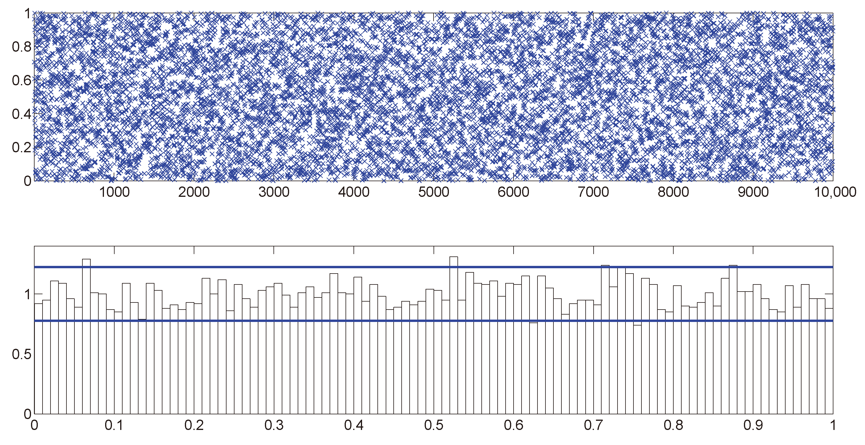
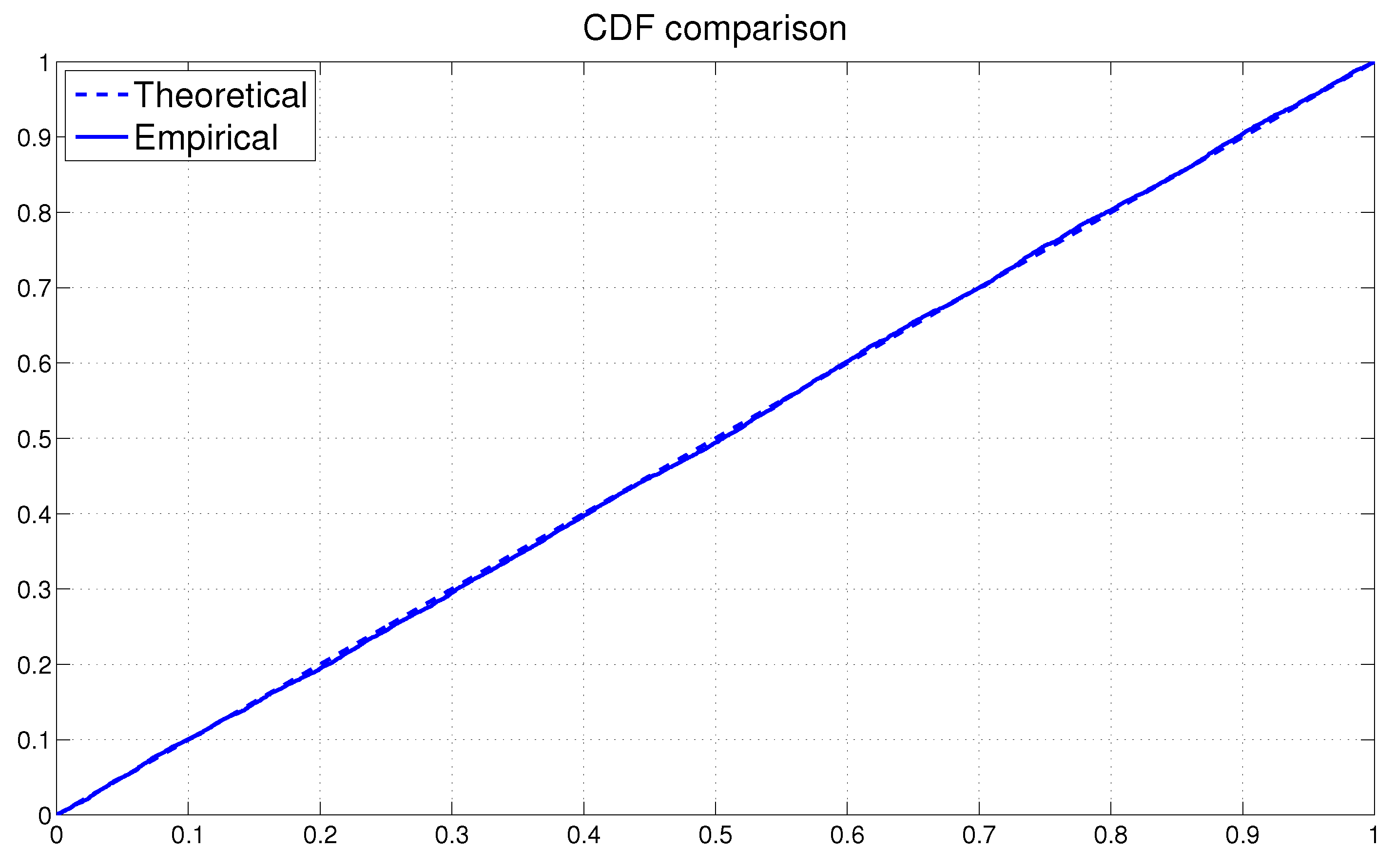
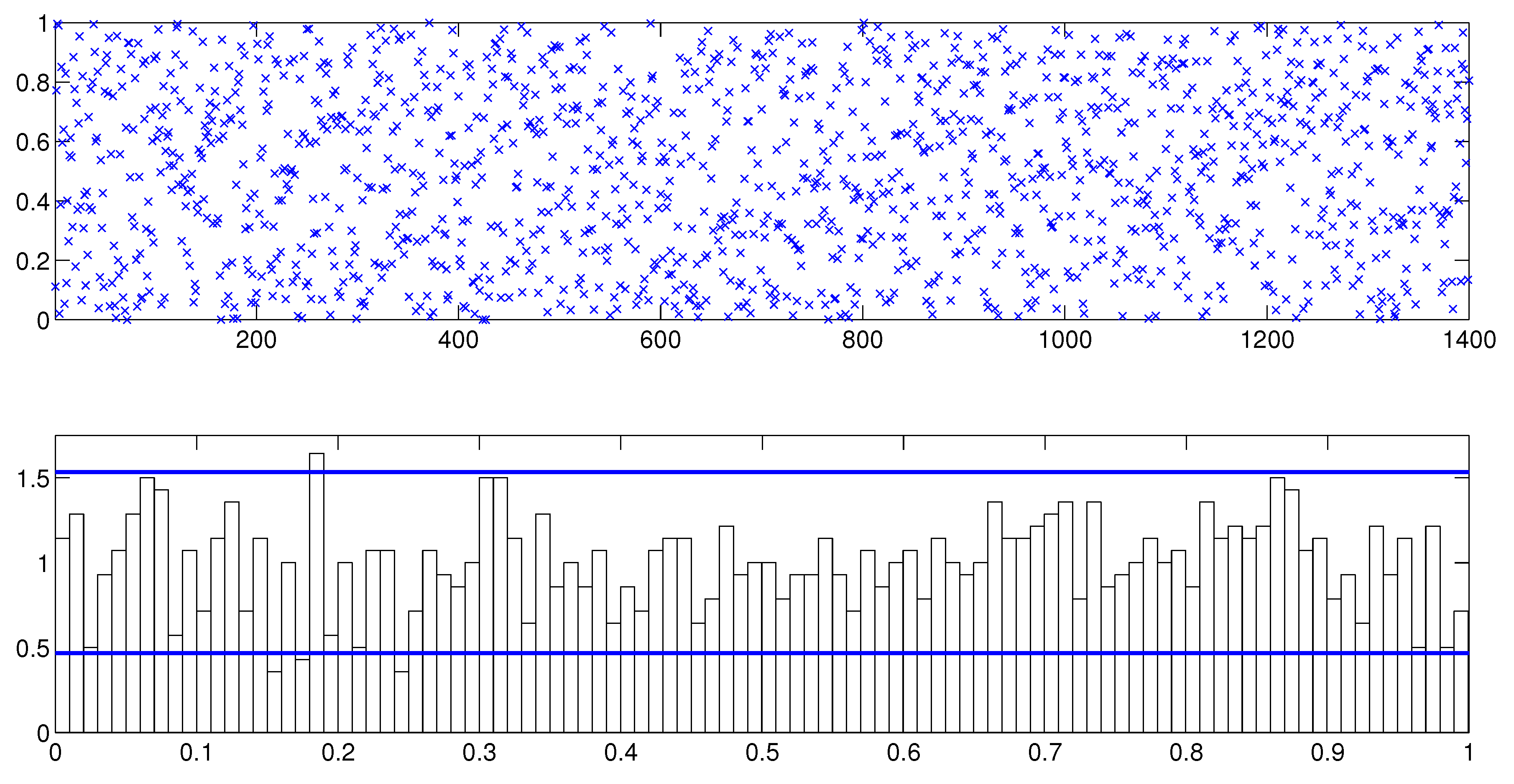
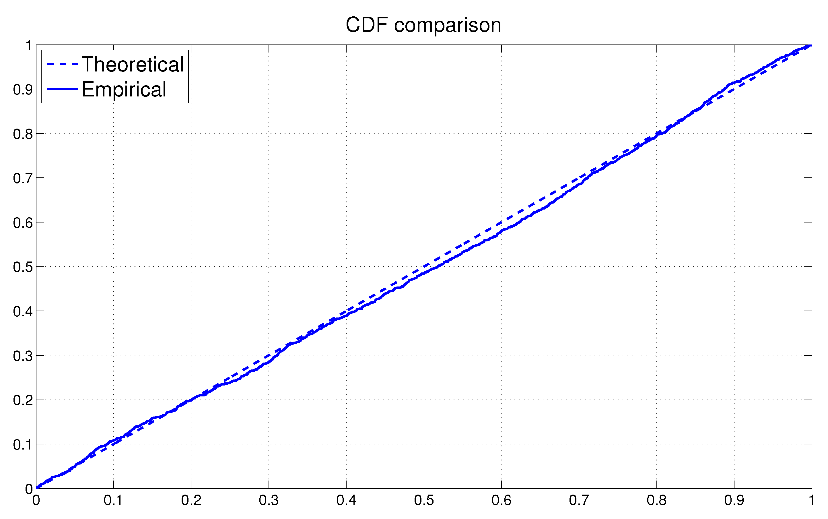
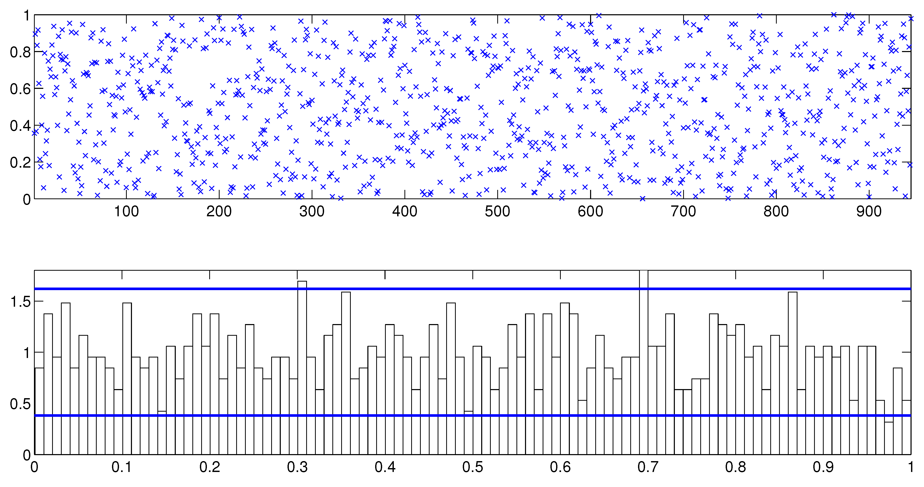
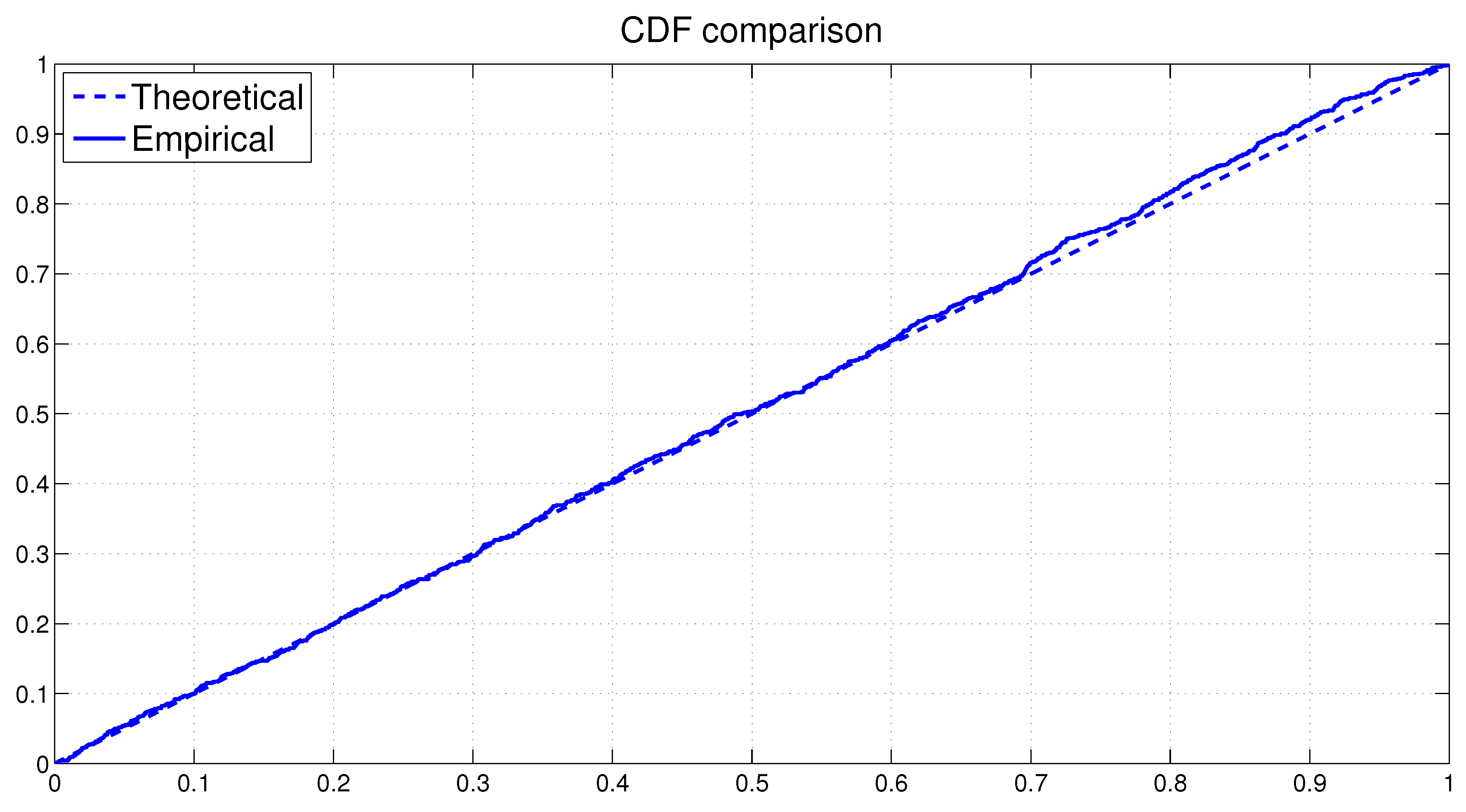
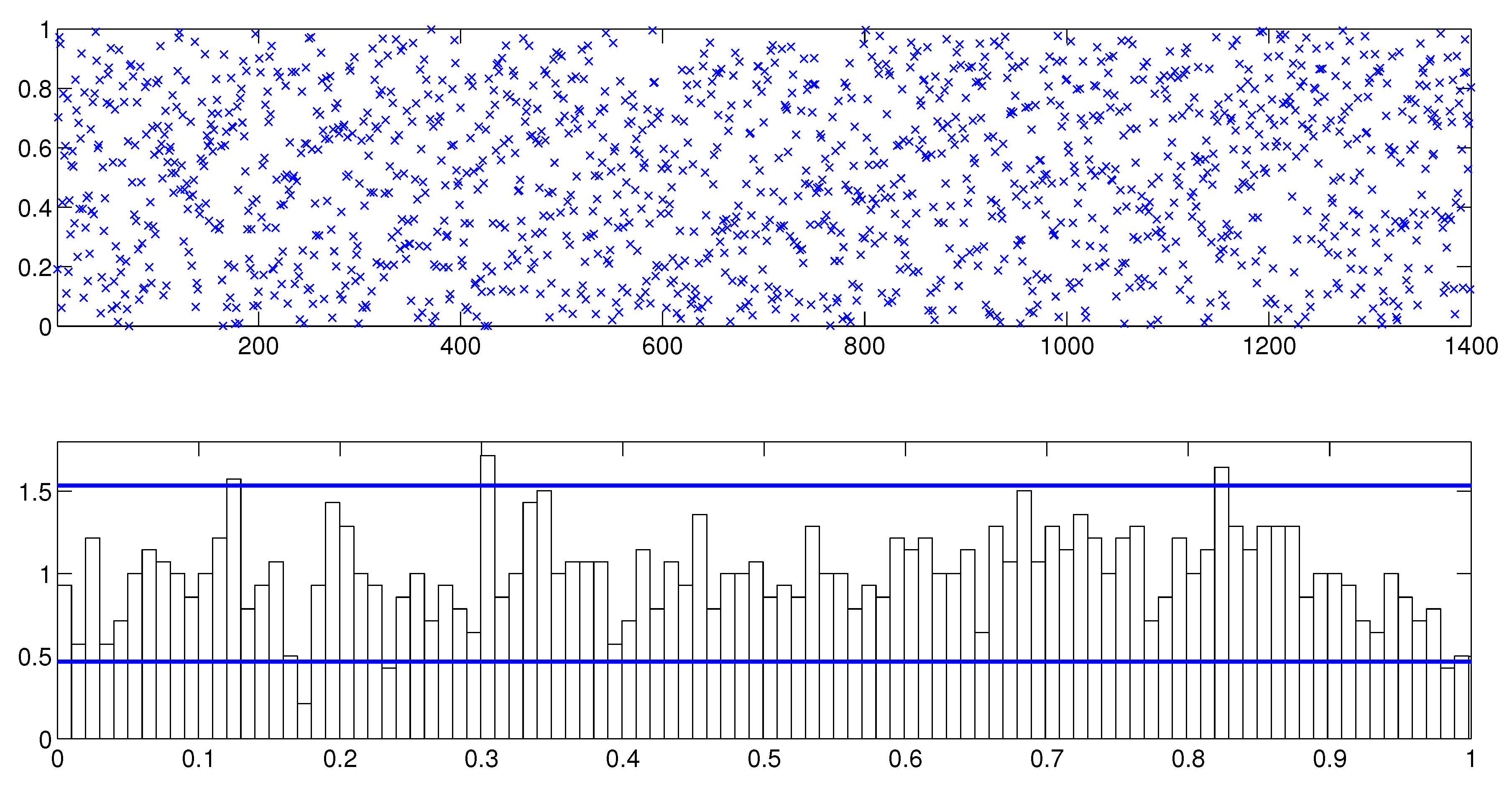
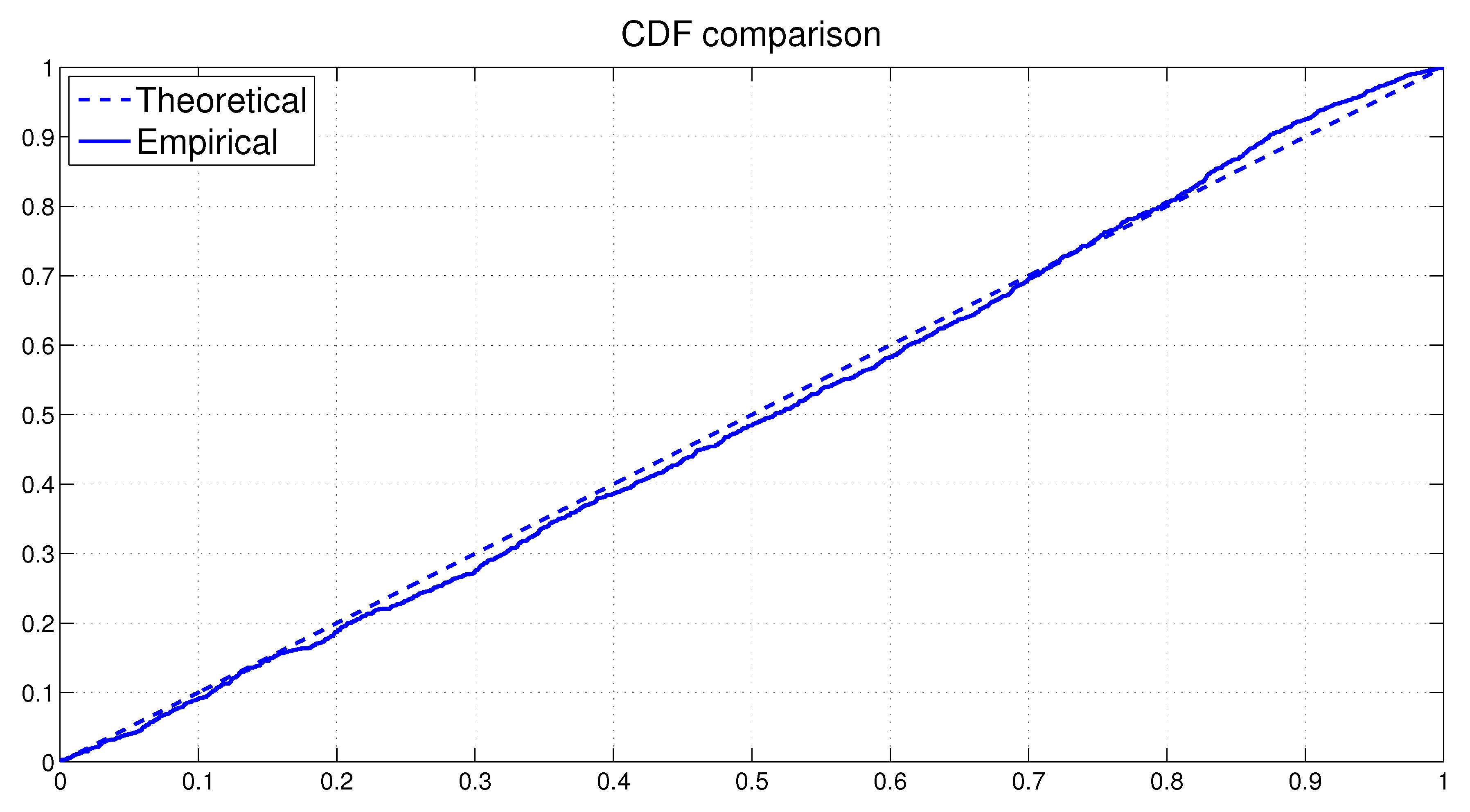
Next we assess the overall fit of the model by analyzing the PITs from the fitted MSASV model. The uniform distribution of $u\left(t\right)$ on the (0, 1) interval is on display in Figure 1 by means of both the scatter plot and the histogram. The two horizontal lines in the histogram plot represent the 95% Bayesian confidence bands, the detail of which calculation can be found in Diebold et al. (1998). The KS test statistic is calculated at 0.0091 with a corresponding p-value of 0.3805. Thus we can not reject the null hypothesis that the PITs are uniformly distributed over the (0, 1) interval at any conventional significance level. In Figure 2 the empirical cumulative distribution function (CDF) of the PITs is plotted together with the theoretical CDF of the uniform distribution $U(0,1)$. The graph reaffirms our earlier claim that the fitted MSASV model agrees well with the simulated return series. From the above comparisons and the result of the KS test we can also draw a conclusion that the proposed MCMC method for the MSASV model fits the simulated return data remarkably well.

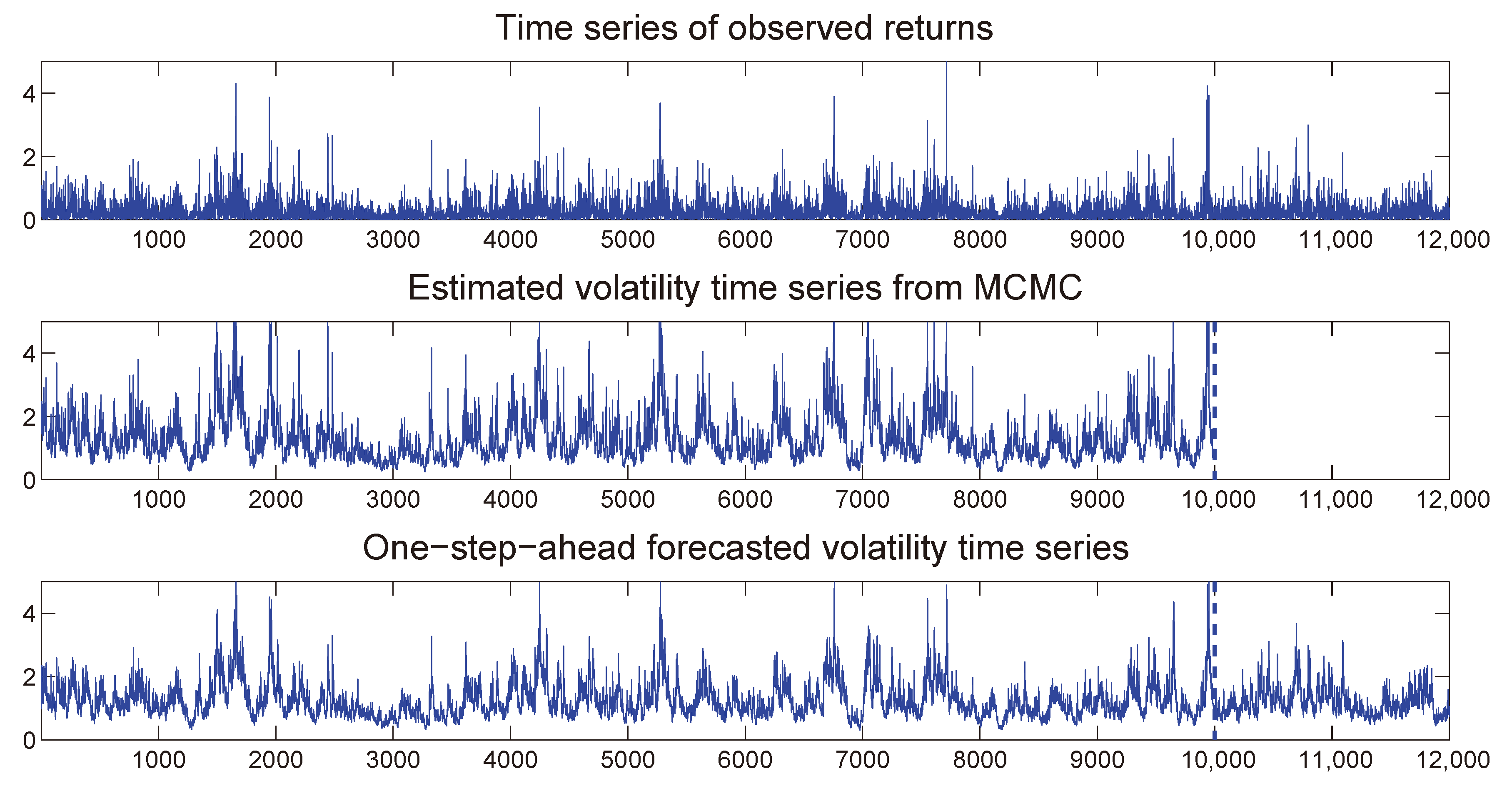
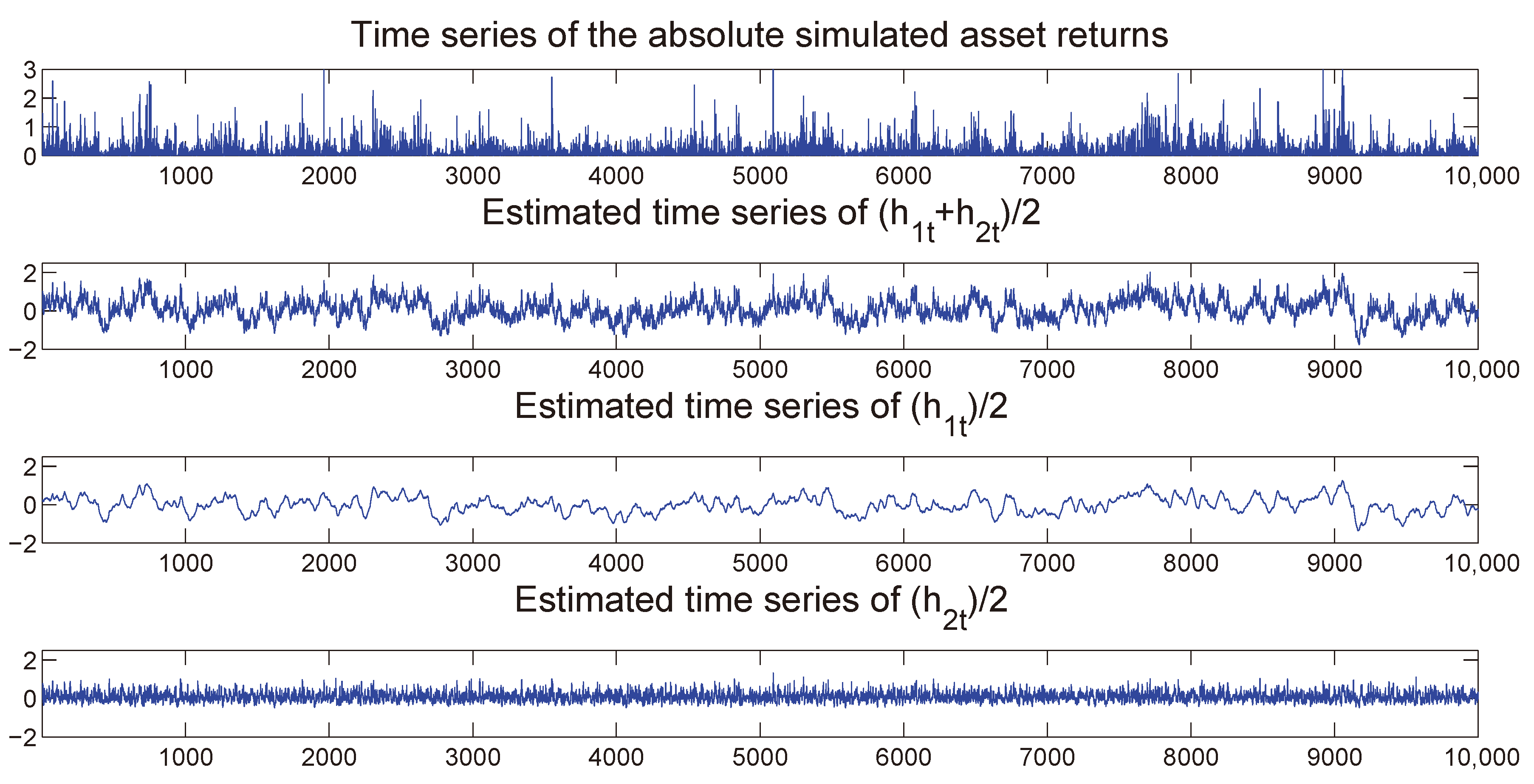
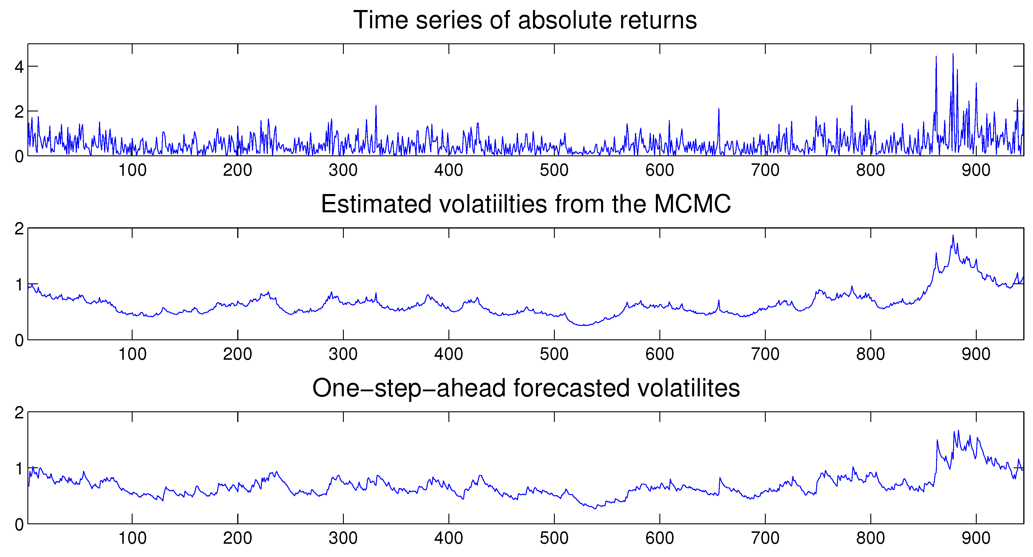
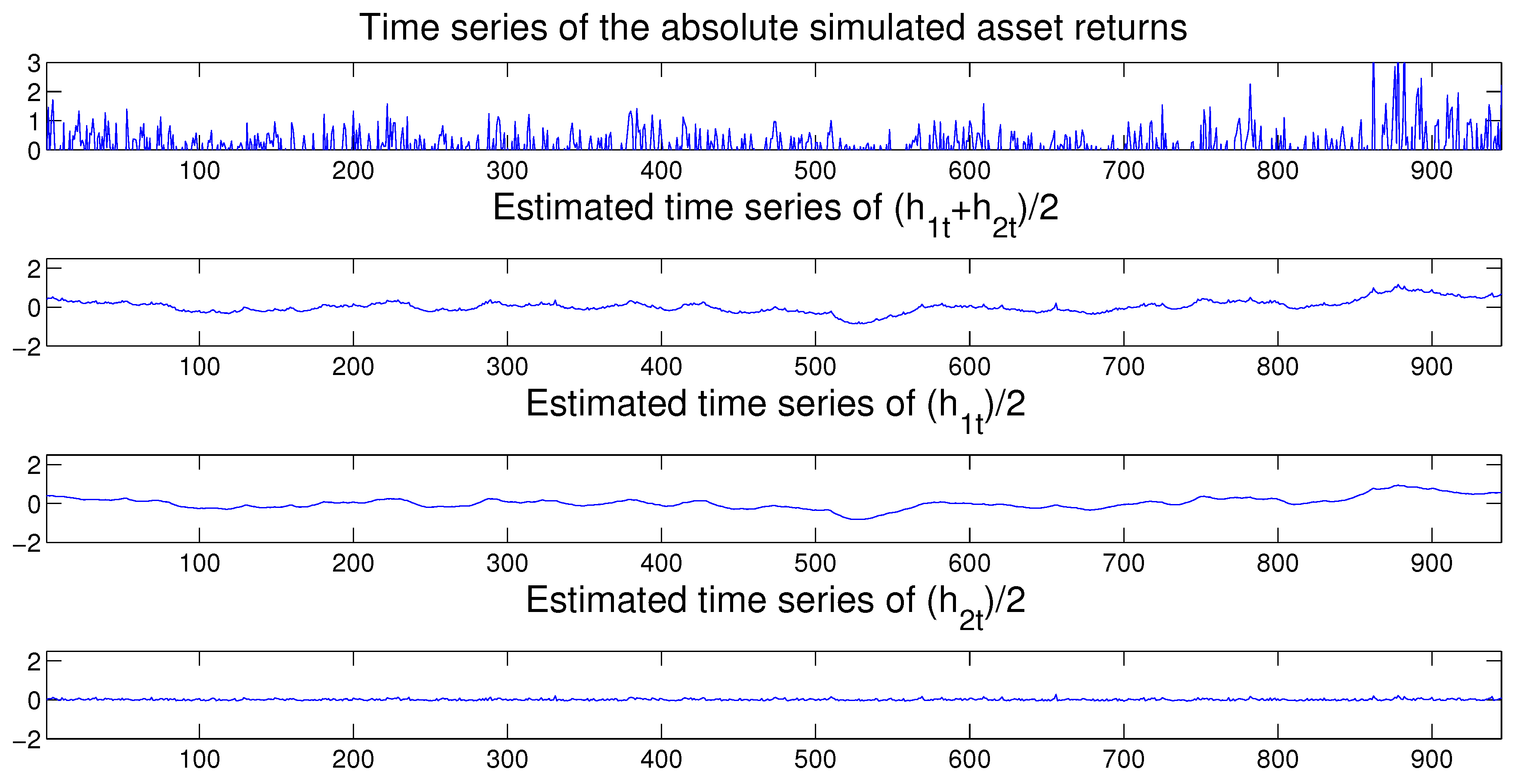
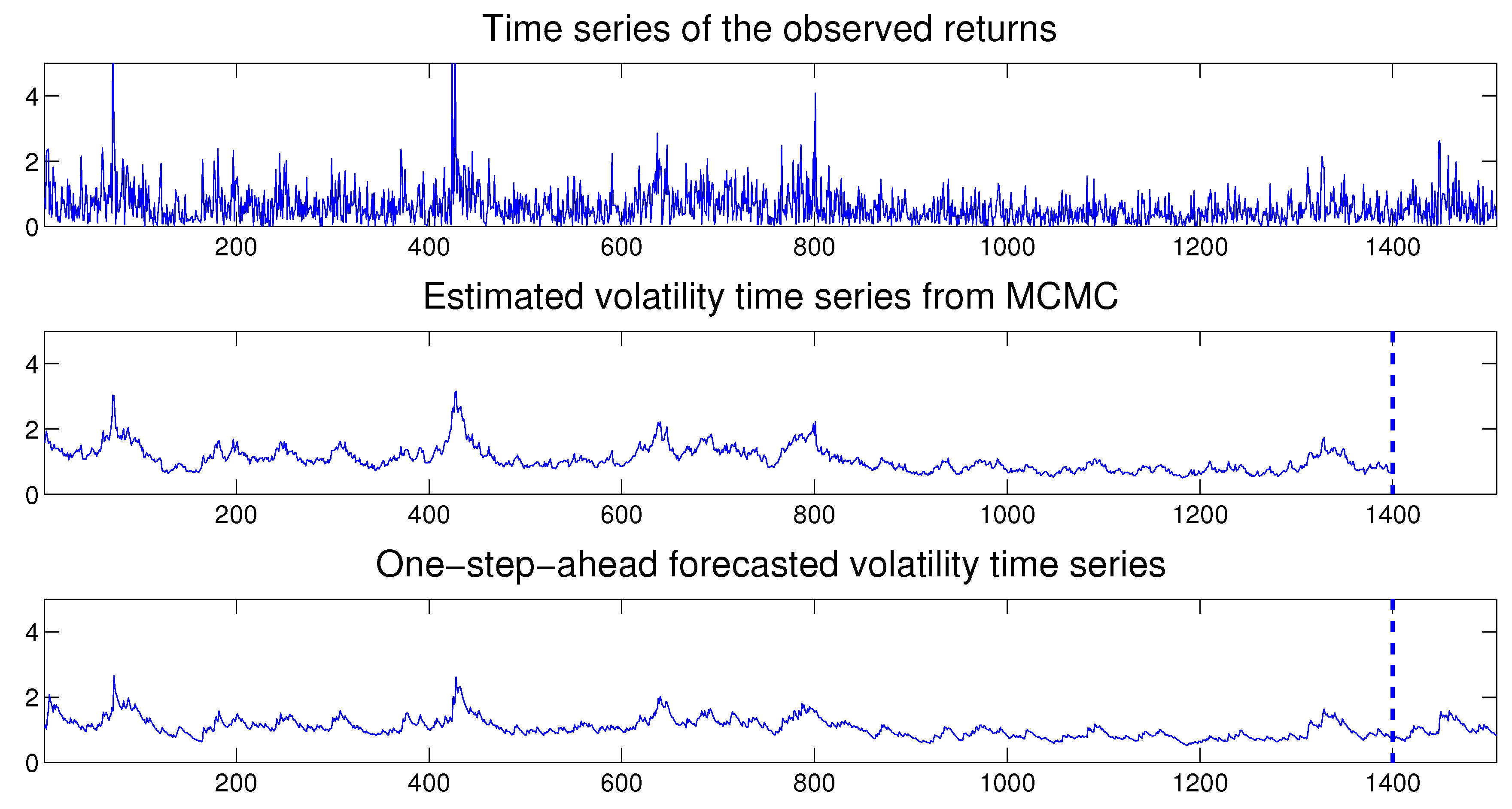
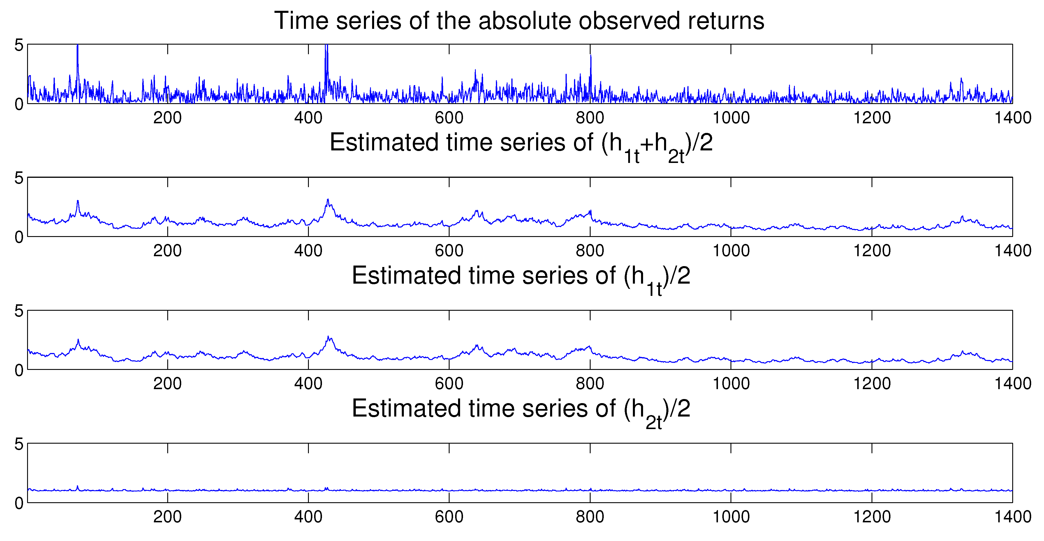
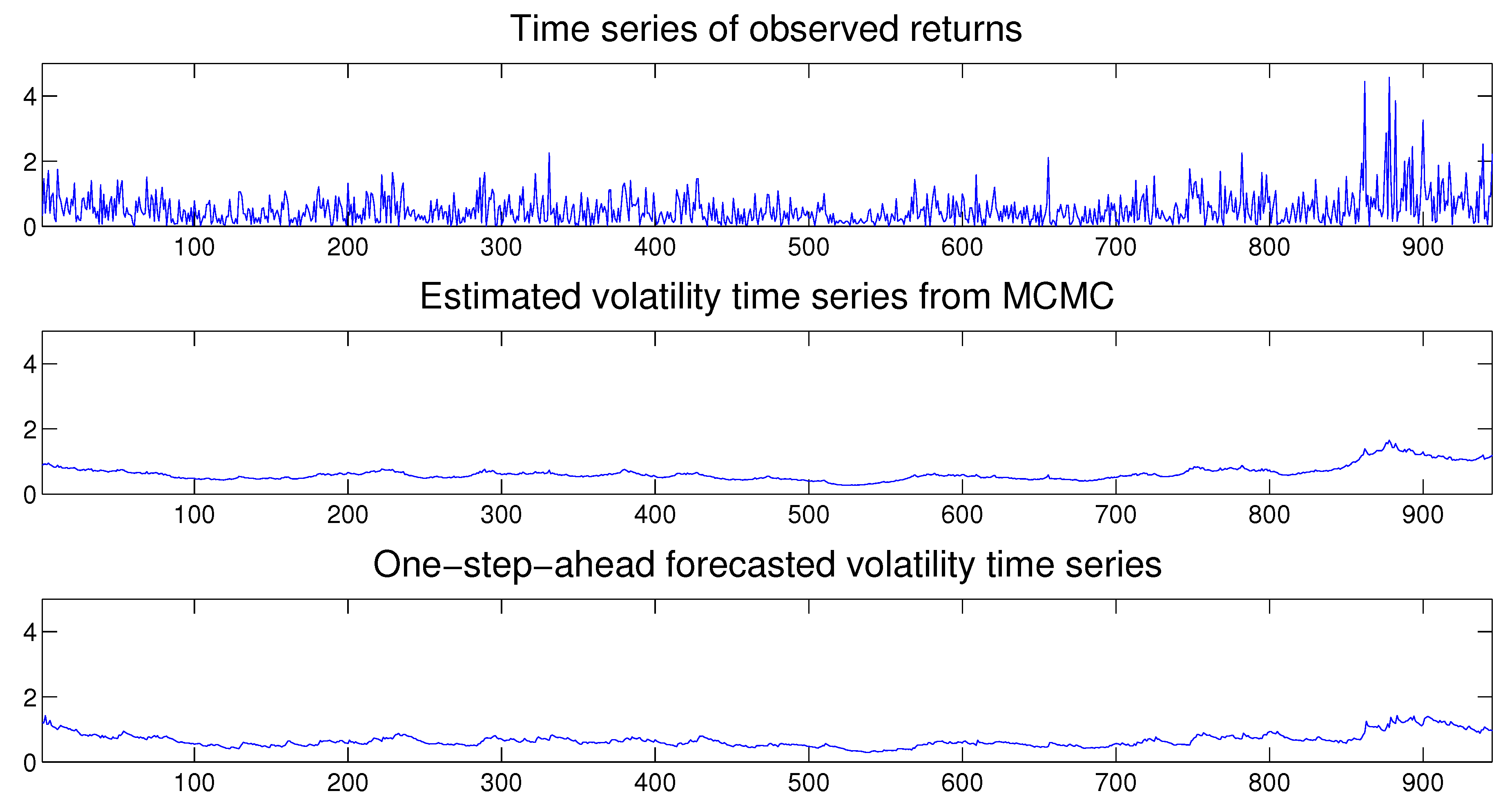
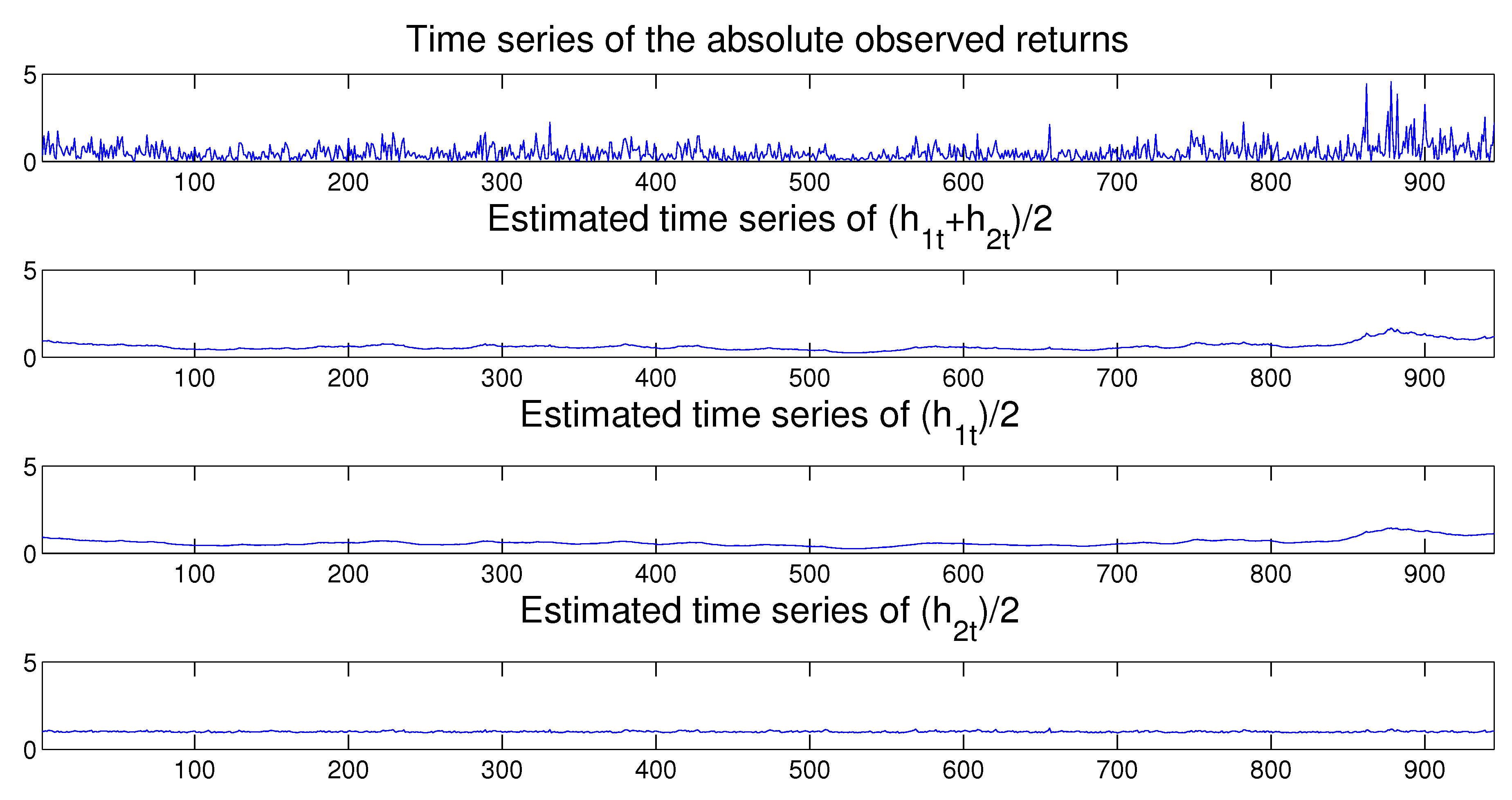
Once the MSASV model has been estimated, we can use the fitted model to perform both the in-sample and out-of-sample one-step ahead volatility predictions. In Figure 3 we compare the absolute value of the simulated returns with the estimated and one-step-ahead in-sample and out-sample predicted volatilities, where the latter is separated by a vertical dotted line at $t=10,000$. We note that the forecasted volatilities resemble very closely the true time series of the absolute value of the simulated returns. Moreover the time series of the estimated two components also compares extremely favorably with the absolute value of the simulated returns on display in Figure 4.

Overall the simulation studies in this section show that the proposed MSASV model and its MCMC algorithm work very well in terms of parameter estimation of the model and are able to capture the two components that shape the dynamics of the volatility of the simulated returns adequately.

5. Empirical Analysis

5.1. The MSASV Model

In this section we apply the proposed MSASV model and its MCMC algorithm to two classic data sets of asset returns with one originating from the exchange market and another one from the equity market. The first data set consists of 945 observations on daily pound/dollar exchange rate from 1 October 1981 to 28 June 1985, called EXC hereafter. The use of this data set allows us to make comparison of our results with those presented in Molina et al. (2010), who use returns from the foreign currency markets. This particular data set from the exchange market has been analyzed in well-known studies such as Harvey et al. (1994); Shephard and Pitt (1997); Meyer and Yu (2000); Skaug and Yu (2008); Yu (2011). Since there are not many observations contained in this data set, we fit all of the available observations by the proposed MSASV model and compare only in-sample predicted volatilities with the estimated and the absolute observed returns. The second data set includes the daily returns of the Australian All Ordinaries stock index, called AUX6. The data set contains 1508 observations from 2 January 2000 to 30 December 2005, excluding weekends and holidays. For a comparison purpose the first 1400 observations are fitted by the proposed MSASV model, and the remaining 108 observations are used for comparison with the estimated and predicted volatilities.

Table 3. Estimated parameters of the MSASV model based on the EXC data.

Parameter	Est.	Std.	HPD CI (95%)
${\varphi }_1$	0.9766	0.0126	(0.9529, 0.9987)
${\rho }_1$	−0.1237	0.1868	(−0.5034,0.2163)
${\sigma }_1$	0.1623	0.0349	(0.0954, 0.2313)
${\varphi }_2$	0.1477	0.3676	(−0.6060, 0.7778)
${\rho }_2$	0.1567	0.1996	(−0.2424, 0.5480)
${\sigma }_2$	0.3162	0.0917	(0.1564, 0.4961)
$\delta$	0.5938	0.0435	(0.5140, 0.6829)

lists the estimated parameters of the MSASV model fitted to the EXC data. Bayesian HPD intervals with standard deviations are also presented in this table. With relatively small standard errors, the HPD intervals contain the parameter estimates of the model. It is worth noting that the leverage/asymmetric effect is estimated with an incorrect expected sign for the second component. Moreover the leverage/asymmetric effect in both components are estimated very imprecisely. This is broadly consistent with the previous findings in the literature on the one-component SV models which shows that the leverage/asymmetric effect is not a prominent feature of the returns in the foreign currency markets.

Our estimates of ${\varphi }_1$ and ${\varphi }_2$ are close to those for the MSSV model reported by Mira and Tierney (2002), which are 0.988 and 0.149 respectively. Importantly the estimation result for ${\varphi }_1$ and ${\varphi }_2$ in Table 3 points to a distinct advantage of the MSASV model vis-a-vis the one-component ASV model for analyzing return data even when the magnitude of the second component (0.1477) is relatively small in magnitude. In particular the MSASV model allows for a better identification of the slower mean-reverting volatility component. We can see this in the results with a more persistently slow mean-reverting component (giving the estimate of ${\varphi }_1$ as 0.9766, which is very close to 1). This is likely to result in a nontrivial impact on the volatility predictions.

The overall model fit can again be assessed by analyzing the PITs from the fitted MSASV model. The uniform distribution of $u\left(t\right)$ on the (0, 1) interval can be visualized in Figure 5 through both the scatter plot and the histogram. As the sample size of the PITs are found to be relatively small, the Bayesian confidence bands of the PITs is relatively much wider as expected. The KS test statistic is recorded at 0.0165 with a p-value of 0.9557. Based on these values we can not reject the null hypothesis that the PITs are uniformly distributed over the (0, 1) interval at any conventional significance level. In Figure 6 the empirical CDF of the PITs is on display together with the theoretical CDF of the $U(0,1)$. The plotted graph is broadly consistent with our earlier finding that the fitted MSASV model compares very favorably with the returns from the foreign currency market. Thus from the above comparisons and the result of the KS test, we can conclude that the proposed MCMC method for the MSASV model fits the return series remarkably well.

In Figure 7 we compare the absolute value of the observed returns with the estimated volatilities and the one-step-ahead in-sample predicted volatilities. The fitted and predicted volatilities appear to track very closely the true time series of the absolute asset returns. Once again the time series of the estimated two components compares very favorably with the absolute value of the observed returns shown in Figure 8.

Next we procedd to carry out the same analysis we had before on the AUX returns data.

Table 4. Estimated parameters of the MSASV model based on the AUX data.

Parameter	Est.	Std.	HPD CI (95%)
${\varphi }_1$	0.9659	0.0101	(0.9460, 0.9840)
${\rho }_1$	−0.7171	0.0849	(−0.8636, −0.5437)
${\sigma }_1$	0.1707	0.0287	(0.1195, 0.2271)
${\varphi }_2$	0.1785	0.3391	(−0.5074, 0.7824)
${\rho }_2$	−0.0633	0.1682	(−0.4046, 0.2766)
${\sigma }_2$	0.3218	0.0829	(0.1581, 0.4756)
v	0.6997	0.0325	(0.6354, 0.7656)

lists the estimated parameters of the MSASV model fitted to the AUX data. Bayesian HPD intervals with standard deviations are also provided in this table. Again with relatively small standard errors, the parameter estimates of the model are included in the constructed HPD intervals. The leverage/asymmetric effect in both factors is estimated this time with a correct expected sign. Moreover its estimate for the first component is quantitatively large and statistically highly significant, while that, for the second component, it is quantitatively small and statistically not significant. As with the EXC data set, even when the estimate of the second component (0.1785) is much smaller in magnitude than that of the first component (0.9659), the use of the MSASV model allows us to better identify the slower mean-reverting volatility component. In particular its estimate is shown to be much more persistent (with the estimate of ${\varphi }_1$ being closer to unity) than the estimate of the second component, and this, in turn, will have a large impact on the overall volatility predictions.

As before the overall model fit can be assessed through the analysis of the PITs from the fitted MSASV model. The uniform distribution of $u\left(t\right)$ on the (0, 1) interval is on display in Figure 9 via both the scatter plot and the histogram. The KS test statistic is calculated at 0.0259 with a p-value of 0.2979. Based on these values we cannot not reject the null hypothesis that the PITs are uniformly distributed over the (0, 1) interval even at the 10% significance level. In Figure 10 the empirical CDF of the PITs is shown together with the theoretical CDF of the Uniform (0, 1). The graph supports our earlier claim that the fitted MSASV model agrees very well with the AUX returns data.

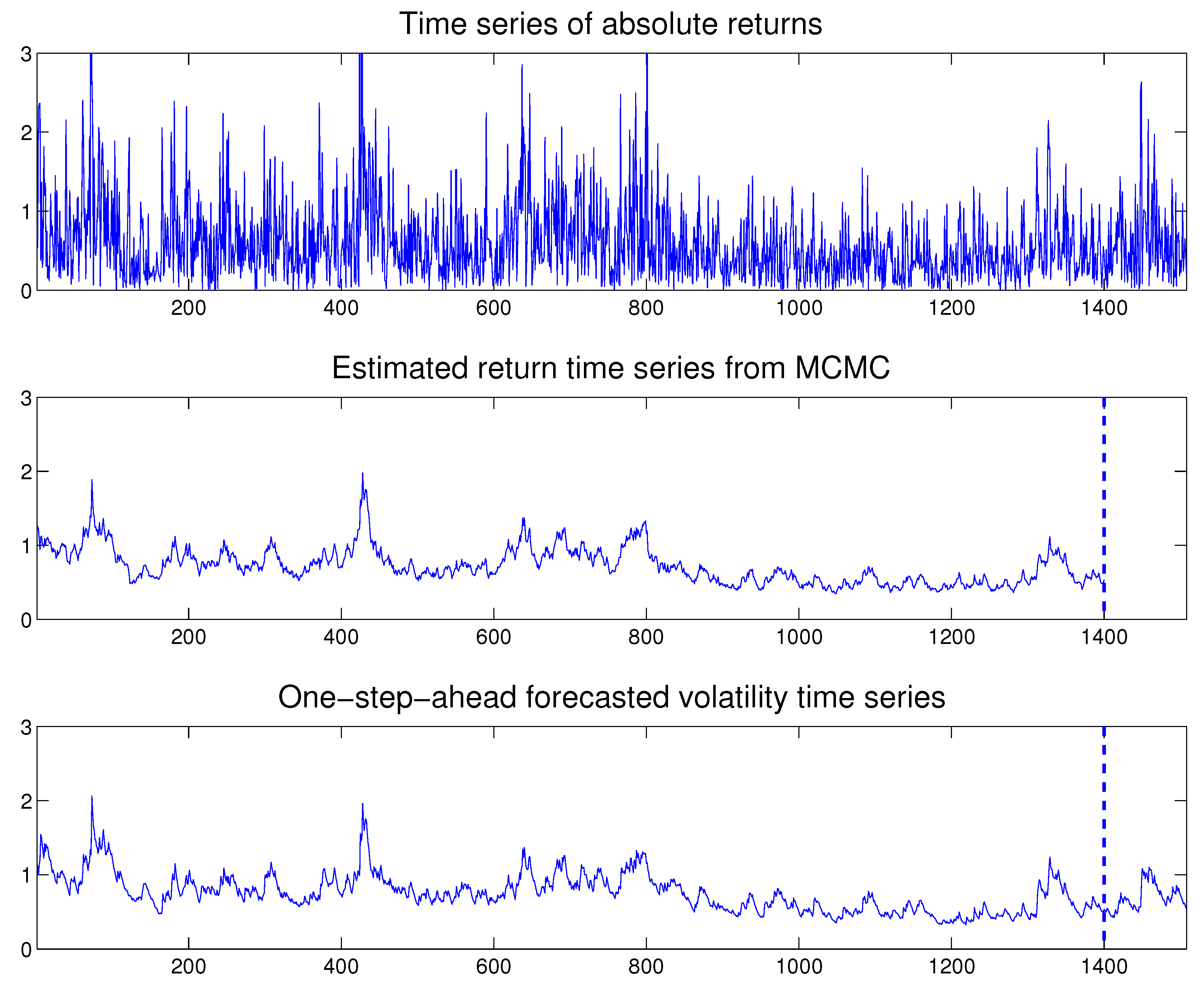
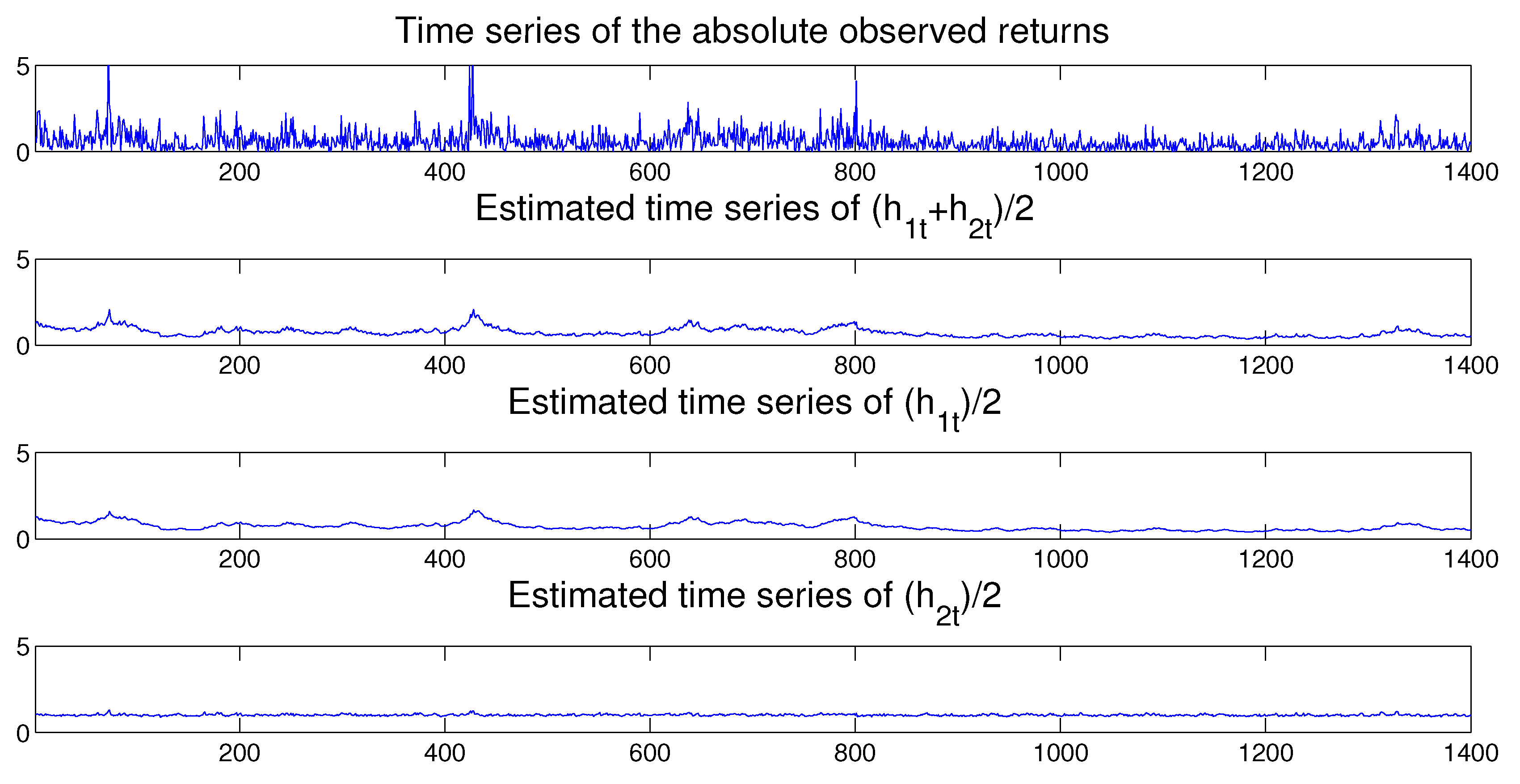
Once the MSASV model has been estimated, as before we can use the fitted model to perform in-sample one-step ahead predictions. In Figure 11 we compare the absolute observed returns with the estimated and one-step-ahead in-sample and out-sample predicted volatilities, where the latter is separated by a vertical dotted line at $t=1400$. The forecasted volatilities appear to resemble closely the true time series of the absolute value of the observed returns. Once again the time series of the estimated two components compares very favorably with the absolute value of the observed returns as shown in Figure 12.

Next we compare the proposed MSASV model with the one-component asymmetric SV (ASV) model where correlation is permitted between the innovation terms of the asset returns and the innovation terms of the latent/unobserved volatility process. The two data sets are also fitted by the one-component ASV model.

Table 5. Model selection for the two data sets.

Panel A: MSASV Model
Criterion	EXC	AUX
$\overline{D}$	1712.8	2943.8
$P_D$	76.92	103.67
DIC	1789.7	3047.5
Panel B: ASV Model
Criterion	EXC	AUX
$\overline{D}$	1753.7	3000.3
$P_D$	44.57	58.06
DIC	1798.2	3058.3

lists the values of $\overline{D}$, $P_D$ and DIC calculated based on the fitted MSASV and one-component ASV models. Based on the calculated DIC values, we conclude that the MSASV model fits the two data sets better and provides evidence of at least two latent/unobserved component volatilities in the dynamics of the asset return data studied in this paper.7

5.2. The MSASV-t Model

In this subsection we fit the heavy/fat tailed MSSV models to the two datasets of the asset returns investigated in Section 5.1.

Table 6. Estimated parameters of the MSASV-t model based on the EXC data.

Parameter	Est.	Std.	HPD CI (95%)
${\varphi }_1$	0.9958	0.0030	(0.9900, 0.9999)
${\rho }_1$	−0.0254	0.0195	(−0.0619, 0.0141)
${\sigma }_1$	0.1085	0.0267	(0.0639, 0.1624)
${\varphi }_2$	0.2621	0.3540	(−0.3741, 0.8909)
${\rho }_2$	0.0498	0.0495	(−0.0495, 0.1437)
${\sigma }_2$	0.2492	0.0847	(0.1113, 0.4137)
v	26.8085	7.5242	(13.8659, 39.9615)

includes the estimated parameters of the MSASV-t model for the EXC data set with the standard deviations and the 95% Bayesian HPD intervals. Estimates of the leverage/asymmetric effect in both factors are quantitatively small and statistically not significant. This again reinforces the previous findings in the literature of the one-component SV models that the leverage/asymmetric effect is not an important feature of the asset returns in the foreign exchange markets.

As in the previous case the assessment of the model fit to the data can be determined by assessing PITs from the fitted MSASV-t model. The uniform distribution of $u\left(t\right)$ on the (0, 1) interval is again visualized in Figure 13 by means of both the scatter plot and the histogram. The KS test statistic is recorded at 0.0283 with a p-value of 0.4294. Based on these values, we can not reject the null hypothesis that the PITs are uniformly distributed over the (0, 1) interval at any conventional significance level. In Figure 14 the empirical CDF of the PITs is plotted together with the theoretical CDF of the Uniform (0, 1). The graph again is shown to be consistent with our earlier assessment that the fitted MSASV-t model compares very favorably with the simulated return data.

In Figure 15 we compare the absolute value of the observed returns with the estimated and predicted volatilities. The fitted and predicted volatilities appear to track very closely the absolute values of the observed asset returns. The time series of the estimated two components also compares quite favorably with the absolute value of the observed returns as presented in Figure 16.

For the AUX return data the estimated parameters, their HPD intervals and related standard deviations are presented in

Table 7. Estimated parameters of the MSASV-t model based on the AUX data.

Parameter	Est.	Std.	HPD CI (95%)
${\varphi }_1$	0.9914	0.0034	(0.9845, 0.9976)
${\rho }_1$	−0.6085	0.0888	(−0.7762, −0.4344)
${\sigma }_1$	0.1220	0.0190	(0.0854, 0.1596)
${\varphi }_2$	0.3320	0.3615	(−0.3887, 0.8987)
${\rho }_2$	−0.3162	0.1909	(−0.6933, 0.0468)
${\sigma }_2$	0.2376	0.0759	(0.1057, 0.3859)
v	24.8652	5.9030	(14.5099, 34.9719)

. The leverage/asymmetric effect in both components in the MSASV-t model is now estimated with the correct expected sign, and quantitatively large as well as statistically highly significant. This suggests that the leverage/asymmetric effect is a distinctly prominent feature of the returns in the equity markets, much in keeping with the findings in the literature on the one-component SV models. As in the previous cases the first and second components of the latent volatility process in this model are estimated significantly at 0.9914 and 0.3320 respectively. As before the fact that the first component of the volatility process has been estimated to be so close to unity gives rise to a better identification of the slow mean-reverting volatility component.

The overall model fit assessment is again conducted by the test of the PITs calculated from the fitted model. The uniform distribution of $u\left(t\right)$ on the (0, 1) interval is on display in Figure 17 through both the scatter plot and the histogram. The KS test statistic is calculated at 0.0362 with a p-value of 0.4867. Based on these values we can not reject the null hypothesis that the PITs are uniformly distributed over the interval (0, 1) at any conventional significance level. In Figure 18 the empirical CDF of the PITs is plotted together with the theoretical CDF of the Uniform (0, 1). The graph simply reinforces our earlier conclusion that the fitted MSASV-t model agrees very strongly with the asset return data.

Figure 19 compares the absolute value of the observed returns with the estimated and one-step-ahead in-sample and out-of-sample predicted volatilities. The predicted volatilities appear again to track very closely the true time series of the absolute returns. In addition the time series of the estimated two factors also compares very favorably with the absolute value of observed returns as illustrated in Figure 20.

As we have done previously in Section 5.1, we compare the proposed MSASV-t model with the heavy-tailed one-factor asymmetric SV (ASV-t) model where the innovation terms of the asset returns have a Student t distribution and are correlated with the innovation terms of the latent volatility process. The two data sets are also fitted by the heavy-tailed one-component ASV-t model, which serves as a benchmark.

Table 8. Model selection based on the two data sets.

Panel A: MSASV-t model
Criterion	EXC	AUX
$\overline{D}$	1762.1	3020.9
$P_D$	34.80	43.77
DIC	1796.90	3064.67
Panel B: ASV-t model
Criterion	EXC	AUX
$\overline{D}$	1768.2	2994.1
$P_D$	38.41	82.47
DIC	1806.61	3076.57

reports the values of $\overline{D}$, $P_D$ and DIC calculated based on the fitted MSASV-t and one-component ASV-t models. It is noted that the MSASV-t model fits the EXC data slightly better than the one-component ASV-t model, while for the AUX data, it fits considerably better than the one-component ASV-t model.

6. Conclusions

In this paper we have systematically studied several extended versions of the multiscale SV model introduced by Molina et al. (2010) in the modeling of the dynamics of the volatility of financial asset returns. The logarithm of conditional volatilities of the asset returns was described by latent/unobserved AR(1) processes with different time scales. In order for the proposed model to capture the heavy/fat tails in the marginal distribution of the asset returns, the innovation terms of the asset returns followed a Student t distribution. Novel MCMC algorithms were developed for the purpose of conducting Bayesian inference of the models. An auxiliary particle filter was also employed to approximate the filtering and prediction distributions of the latent/unobserved states of the models when we calculated the models’ likelihoods and performed volatility predictions. In this paper, we also allowed for a nontrivial correlation structure between the innovation of the mean equation and those of the latent factor processes, which can be interpreted as the leverage/asymmetric effect, much in keeping with the literature on the one-component SV models. However, we did not allow for a correlation structure to exist among the innovation terms of latent/unobserved AR(1) processes. This was done for the reason of computational tractability and to ensure model identifiability. This is a limitation of the present study and represents an important issue to be considered as future research. We briefly discuss this issue in Appendix A and show how it may be resolved if we are willing to impose additional restrictions on the model, in particular on the noise/innovation terms driving the process of the various volatility components in the model.

References

- Aguilar, Omar, and Mike West. 2000. Bayesian Dynamic Factor models and variance matrix discounting for portfolio allocation. Journal of Business and Economic Statistics 18: 338–57. [Google Scholar]
- Akaike, Hirotugu. 1987. Factor Analysis and AIC. Psychometrika 52: 317–32. [Google Scholar] [CrossRef]
- Alizadeh, Sasan, Michael W. Brandt, and Francis X. Diebold. 2002. Range-Based Estimation of Stochastic Volatility Models. Journal of Finance 57: 1047–91. [Google Scholar] [CrossRef] [Green Version]
- Bauwens, Luc, and Michel Lubrano. 1998. Bayesian inference on GARCH models using the Gibbs sampler. Econometrics Journal 1: C23–46. [Google Scholar] [CrossRef]
- Berg, Andreas, Renate Meyer, and Jun Yu. 2004. Deviance Information Criterion for Comparing Stochastic Volatility Models. Journal of Business and Economic Statistics 22: 107–20. [Google Scholar] [CrossRef]
- Black, Fischer. 1976. Studies of Stock Price Volatility Changes. Paper presented at the Business and Economics Section of the American Statistical Association, Washington, DC, USA, August 25–26; pp. 177–81. [Google Scholar]
- Chernov, Mikhail, A. Ronald Gallant, Eric Ghysels, and George Tauchen. 2003. Alternative Models for Stock Price Dynamics. Journal of Econometrics 116: 225–57. [Google Scholar] [CrossRef] [Green Version]
- Chib, Siddhartha, and Edward Greenberg. 1995. Understanding the Metropolis–Hastings algorithm. The American Statistician 49: 327–35. [Google Scholar]
- Chib, Siddhartha, Federico Nardari, and Neil Shephard. 2002. Markov Chain Monte Carlo Methods for Generalized Stochastic Volatility Models. Journal of Econometrics 108: 281–316. [Google Scholar] [CrossRef]
- Chib, Siddhartha, Federico Nardari, and Neil Shephard. 2006. Analysis of High Dimensional Multivariate Stochastic Volatility Models. Journal of Econometrics 134: 341–71. [Google Scholar] [CrossRef]
- Chib, Siddhartha, Yasuhiro Omori, and Manabu Asai. 2009. Multivariate Stochastic Volatility. Handbook of Financial Time Series; Berlin/Heidelberg, Germany: Springer. [Google Scholar]
- Christie, Andrew A. 1982. The Stochastic Behavior of Common Stock Variances: Value, leverage, and Interest Rate Effects. Journal of Financial Economics 10: 407–32. [Google Scholar] [CrossRef]
- Diebold, Francis X., Todd A. Guther, and Anthony S. Tay. 1998. Evaluating Density Forecasts with Applications to Financial Risk Management. International Economic Review 39: 863–83. [Google Scholar] [CrossRef] [Green Version]
- Geweke, John. 1993. Bayesian treatment of the independent Student t linear model. Journal of Applied Econometrics 8: 19–40. [Google Scholar] [CrossRef]
- Griffin, Jim E., and Mark F. J. Steel. 2010. Bayesian Inference with Stochastic Volatility Models Using Continuous Superpositions of Non-Gaussian Ornstein–Uhlenbeck Processes. Computational Statistics and Data Analysis 54: 2594–608. [Google Scholar] [CrossRef] [Green Version]
- Harvey, Andrew C., and Neil Shephard. 1996. Estimation of an Asymmetric Stochastic Volatility Model for Asset Returns. Journal of Business & Economic Statistics 14: 429–34. [Google Scholar]
- Harvey, Andrew C., Esther Ruiz, and Neil Shephard. 1994. Multivariate Stochastic Variance Models. Review of Economic Studies 61: 247–64. [Google Scholar] [CrossRef] [Green Version]
- Jacquier, Eric, Nicholas G. Polson, and Peter E. Rossi. 1994. Bayesian analysis of stochastic volatility models (with discussion). Journal of Business & Economic Statistics 12: 371–417. [Google Scholar]
- Jacquier, Eric, Nicholas G. Polson, and Peter E. Rossi. 2004. Bayesian Analysis of Stochastic Volatility Models with Fat-tails and Correlated Errors. Journal of Econometrics 122: 185–212. [Google Scholar] [CrossRef]
- Jensen Mark J., John M. Maheu. 2010. Bayesian Semiparametric Stochastic Volatility Modeling. Journal of Econometrics 157: 306–16. [Google Scholar] [CrossRef] [Green Version]
- Jensen, Mark J., and John M. Maheu. 2014. Estimating a Semiparametric Asymmetric Stochastic Volatility Model with a Dirichlet Process Mixture. Journal of Econometrics 178, Pt 3: 523–38. [Google Scholar] [CrossRef] [Green Version]
- Kalli, Maria, and Jim E. Griffin. 2015. Flexible modelling of dependence in volatility processes. Journal of Business and Economic Statistics 33: 102–13. [Google Scholar] [CrossRef] [Green Version]
- Kim, Sangjoon, Neil Shephard, and Siddhartha Chib. 1998. Stochastic Volatility: Likelihood Inference and Comparison with ARCH Models. Review of Economic Studies 65: 361–93. [Google Scholar] [CrossRef]
- LeBaron, Blake. 2001. Stochastic Volatility as a Simple Generator of Apparent Financial Power Laws and Long Memory. Quantitative Finance 1: 621–31. [Google Scholar] [CrossRef]
- Li, Yong, Jun Qing Yu, and Tao Zeng. 2014. Robust Deviance Information Criterion for Latent Variable Models, Singapore Management University. Available online: http://www.mysmu.edu/faculty/yujun/Research/BCE36.pdf (accessed on 26 September 2016).
- Lopes Hedibert F., Nicholas G. Polson. 2010. Bayesian Inference for Stochastic Volatility Modeling. In Rethinking Risk Measurement and Reporting. Volume 1, Uncertainty, Bayesian Analysis and Expert Judgment. Edited by Bocker Klaus. London: RiskBooks, pp. 515–51. [Google Scholar]
- Men, Zhongxian, Adam W. Kolkiewicz, and Tony S. Wirjanto. 2016. Bayesian Analysis of Threshold Stochastic Volatility Models. Journal of Forecasting 35: 462–76. [Google Scholar]
- Men, Zhongxian, and Tony S. Wirjanto. 2018. A New Variant of Estimation Approach to Asymmetric Stochastic Volatility Model. A special issue on Volatility of Prices of Financial Assets. Quantitative Finance and Economics 2: 325–47. [Google Scholar] [CrossRef]
- Men, Zhongxian, Don McLeish, Adam W. Kolkiewicz, and Tony S. Wirjanto. 2016. Comparison of Asymmetric Stochastic Volatility Models under Different Correlation Structures. Journal of Applied Statistics 44: 1350–68. [Google Scholar] [CrossRef]
- Meyer, Renate, and Jun Yu. 2000. BUGS for a Bayesian Analysis of Stochastic Volatility Models. Econometrics Journal 3: 198–215. [Google Scholar] [CrossRef]
- Mira, Antonietta, and Tierney Luke. 2002. Efficiency and convergence properties of slice samplers. Scandinavian Journal of Statistics 29: 12. [Google Scholar] [CrossRef]
- Molina, German, Chuan-Hsiang Han, and Jean-Pierre Fouque. 2010. McMC Estimation of Multiscale Stochastic Volatility Models. In Handbook of Quantitative Finance and Risk Management. Boston: Springer, chp. 71. pp. 1109–20. [Google Scholar]
- Neal, Radford M. 2003. Slice sampling. The Annals of Statistics 31: 705–67. [Google Scholar] [CrossRef]
- Pitt, Michael K., and Neil Shephard. 1999. Filtering via Simulation: Auxiliary Particle Filters. Journal of the American Statistical Association 94: 590–99. [Google Scholar] [CrossRef]
- Roberts Gareth O., Jeffrey S. Rosenthal. 1999. Convergence of slice sampler Markov chains. Journal of the Royal Statistical Society. Series B (Statistical Methodology) 61: 643–60. [Google Scholar] [CrossRef]
- Roberts, Gareth O., Omiros Papaspiliopoulos, and Petros Dellaportas. 2004. Bayesian Inference for Non-Gaussian Ornstein–Uhlenbeck Stochastic Volatility Processes. Journal of the Royal Statistical Society, series B (Statistical Methodology) 66: 369–93. [Google Scholar] [CrossRef]
- Schwarz, Gideon. 1978. Estimating the Dimension of a Model. Annals of Statistics 6: 461–64. [Google Scholar] [CrossRef]
- Shephard, Neil, and Michael K. Pitt. 1997. Likelihood Analysis of non-Gaussian Measurement Time Series. Biometrika 84: 653–67. [Google Scholar] [CrossRef]
- Skaug, Hans J., and Jun Yu. 2008. Automated Likelihood Based Inference for Stochastic Volatility Models. Working Paper. Singapore: Singapore Management University. [Google Scholar]
- Spiegelhalter, David J., Nicola G. Best, Bradley P. Carlin, and Angelika van der Linde. 2002. Bayesian Measures of Model Complexity and Fit (with discussion). Journal of the Royal Statistical Society, Series B 64: 583–639. [Google Scholar] [CrossRef] [Green Version]
- Taylor, Stephen J. 1986. Modeling Financial Time Series. Chichester: Wiley. [Google Scholar]
- Yu, Jun, Zhenlin Yang, and Xibin Zhang. 2006. A class of nonlinear stochastic volatility models and its implication for pricing currency options. Computational Statistics and Data Analysis 51: 2218–31. [Google Scholar] [CrossRef] [Green Version]
- Yu, Jun. 2011. Simulation-Based Estimation Methods for Financial Time Series Models. In Handbook of Computational Finance. Edited by Duan Jin-Chuan, Wolfgang Karl Hardle and James E. Gentle. Berlin and Heidelberg: Springer, chp. 15. pp. 401–35. [Google Scholar]
- Zhang, Xibin, and Maxwell L. King. 2008. Box-Cox Stochastic Volatility Models with Heavy Tails and Correlated Errors. Journal of Empirical Finance 15: 549–66. [Google Scholar] [CrossRef] [Green Version]
Figure 1.
Analysis of the PITs from the MSASV model based on the simulated return data. The top panel shows the scatter plot of while the bottom panel shows the histogram of .
Figure 2.
Comparison between the CDF of the uniform distribution and the empirical CDF of the PITs from the MSASV model based on the simulated return data.
Figure 3.
Comparison between the absolute returns and the one-step-ahead forecasted volatilities under the MSASV model based on the simulated return data.
Figure 4.
Time series of the absolute returns (first panel). Posterior mean of (second panel). Posterior mean of slow mean reverting of (third panel) and the posterior mean of fast mean reverting of (fourth panel) based on the simulated return data.
Figure 5.
Analysis of the PITs from the MSASV model based on EXC data. The top panel shows the scatter plot of while the bottom panel shows the histogram of .
Figure 6.
Comparison between the CDF of the uniform distribution and the empirical CDF of the PITs from the MSASV model based on the EXC data.
Figure 7.
Comparison between the absolute returns and the one-step-ahead forecasted volatilities under the MSASV model based on the EXC data.
Figure 8.
Time series of the absolute returns (first panel). Posterior mean of (second panel). Posterior mean of slow mean reverting of (third panel) and the posterior mean of fast mean reverting of (fourth panel) based on the EXC data.
Figure 9.
Analysis of the PITs from the MSASV model based on AUX data. The top panel shows the scatter plot of while the bottom panel shows the histogram of .
Figure 10.
Comparison between the CDF of the uniform distribution and the empirical CDF of the PITs from the MSASV model based on the AUX data.
Figure 11.
Comparison between the absolute returns and the one-step-ahead forecasted volatilities under the MSASV model based on the AUX data.
Figure 12.
Time series of the absolute returns (first panel). Posterior mean of (second panel). Posterior mean of slow mean reverting of (third panel) and the posterior mean of fast mean reverting of (fourth panel) based on the AUX data.
Figure 13.
Analysis of the PITs from the MSASV-t model based on EXC data. The top panel shows the scatter plot of while the bottom panel shows the histogram of .
Figure 14.
Comparison between the CDF of the uniform distribution and the empirical CDF of the PITs from the MSASV-t model based on the EXC data.
Figure 15.
Comparison between the absolute returns and the one-step-ahead forecasted volatilities under the MSASV-t model based on the EXC data.
Figure 16.
Time series of the absolute value of asset returns (first panel). Posterior mean of (second panel). Posterior mean of slow mean reverting of (third panel) and the posterior mean of fast mean reverting of (fourth panel) based on the MSASV-t model for the EXC data.
Figure 17.
Analysis of the PITs from the MSASV-t model based on AUX data. The top panel shows the scatter plot of while the bottom panel shows the histogram of .
Figure 18.
Comparison between the CDF of the uniform distribution and the empirical CDF of the PITs from the MSASV-t model based on the AUX data.
Figure 19.
Comparison between the absolute returns and the one-step-ahead forecasted volatilities under the MSASV-t model based on the AUX data.
Figure 20.
Time series of the absolute value of asset returns (first panel). Posterior mean of (second panel). Posterior mean of slow mean reverting of (third panel) and the posterior mean of fast mean reverting of (fourth panel) based on the MSASV-t model for the AUX data.