
Global Index on Financial Losses Due to Crime in the United States


1
Department of Mathematics and Statistics, Texas Tech University, Lubbock, TX 79409, USA
2
College of Business and Public Administration, Drake University, Des Moines, IA 50311, USA
*
Author to whom correspondence should be addressed.
J. Risk Financial Manag. 2021, 14(7), 315; https://0-doi-org.brum.beds.ac.uk/10.3390/jrfm14070315
Submission received: 7 May 2021
/
Revised: 5 July 2021
/
Accepted: 6 July 2021
/
Published: 9 July 2021
(This article belongs to the Special Issue Mathematical and Empirical Finance)
Abstract
:Despite the potential importance of crime rates in investments, there are no indices dedicated to evaluating the financial impact of crime in the United States. As such, this paper presents an index-based insurance portfolio for crime in the United States by utilizing the financial losses reported by the Federal Bureau of Investigation. The objective of our paper is to introduce new risk hedging financial contracts for crime, consistent with dynamic asset pricing. Underlying the index, we hedge the investments by issuing marketable European call and put options and providing risk budgets. These budgets show that real estate, ransomware, and government impersonation are the main risk contributors in our index. Next, we evaluate the performance of our index via stress testing to determine its resilience to economic crisis. Of all the factors considered in this study, unemployment rate has the potential to demonstrate the highest systemic risk to the portfolio. Our portfolio will help investors envision risk exposure in the market, gauge investment risk based on their desired risk level, and hedge strategies for potential losses due to economic crashes. In conclusion, we provide a basis for the securitization of insurance risk from certain crimes that could forewarn investors to transfer their risk to capital market investors.
1. Introduction
The United States spends between 2% and 6% of the nation’s gross domestic product on crime victimization (Lugo et al. 2019). The Department of Justice reported that federal, state, and local governments spent more than $280 billion on criminal justice, including police protection, the court system, and prisons in 2012 (United States Department of Justice 2019). In addition, the financial losses due to crime can be viewed as significant dynamic factors that can influence and even shock the financial market in the United States (Chalfin 2015; Maure 2017; McCollister et al. 2010). In 2019, 6,925,677 property crimes were reported nationwide where the victims suffered losses estimated at $15.8 billion (Hindelang 1974). Over the years, cybercrime has grown rapidly with the expansion of internet usage and e-commerce and has contributed immensely to security threats in the United States (Anderson et al. 2013). In 2019, the Internet Crime Complaint Center of the Federal Bureau of Investigation reported 467,361 complaints—an average of nearly 1300 every day—with financial losses of more than $3.5 billion to individual and business victims (Internet Crime Complaint Center 2019). Determining the economic impacts caused by these crimes could help policymakers assess the level of systemic risk related to future compensations (Lugo et al. 2019). Our research provides new risk hedging financial contracts based on an examination of the economic impact of all emerging crime types in the United States.
One method of mitigating the economic impact includes crime insurance and dishonesty bonds. These insurance policies are available to business owners and help cover the financial losses caused by criminal acts such as fraud, embezzlement, forgery, robbery, and theft (Weissman 2017). While crime insurance only compensates losses caused by employee theft, dishonesty bonds also cover customer-related theft. However, in these types of insurance contracts, it is not clear if the underlying model is free of arbitrage, that is to say, whether the insurance policy is fair or not. Provided the underlying models in these two approaches are free of arbitrage, the valuation of risk hedging derivatives can be done according to the dynamic asset pricing theory. Therefore, the goal of our paper is to introduce new risk hedging financial contracts for crime, consistent with dynamic asset pricing (rational finance) that are transparent to investors.
We propose a reliable and dynamic aggregate index for crime based on economic factors to provide a basis for the securitization of insurance risk. Taking all the available data in uniform crime reports and internet crime reports published by the Federal Bureau of Investigation (Internet Crime Complaint Center 2019; United States Department of Justice 2019), we model the economic damages generated by property crimes and cybercrimes. Then, we propose a portfolio based on their financial losses and validate it by implementing value at risk backtesting models (Nieppola 2009).
We hedge the investments underlying the portfolio by assessing the level of future systemic risk using two methods. First, we issue marketable financial contracts in our portfolio, the European call and put options, to help the investors strategize buying call options and selling put options in our portfolio based on their desired risk level. Second, we hedge the investments by diversifying risk to each type of crime based on tail risk and center risk measures. According to the estimated risk budgets, real estate, ransomware, and government impersonation are the largest contributors to the risk in our portfolio. These findings will help investors to envision the amount of risk exposure with financial planning on our portfolio.
Preexisting literature (Lieberman and Smith 1986) outlines that poverty indicators are positively correlated with the crime rate. Other studies (Raphael and Winter-Ebmer 2001; Wadsworth 2001) have shown that unemployment has a significant positive effect on property crime rates. Using this research as a foundation, we evaluate the performance of our index with respect to these economic factors to determine its strength and resilience to the economic crisis. Within our portfolio, the unemployment rate potentially demonstrates a high systemic risk compared to the poverty indicators. That is, our key findings are consistent with the aforementioned studies (Lieberman and Smith 1986; Raphael and Winter-Ebmer 2001; Wadsworth 2001) and also provide a quantitative comparison between the effects of economic factors used in those studies. This will help insurers gauge investment risk in our portfolio based on their desired risk level and hedge strategies for potential losses due to economic crashes.
There have been numerous studies that introduce indices based on crime rates which take the number of crimes into account. The two most common examples of these indices are the Uniform Crime Reports (UCR) index and the Sellin–Wolfgang index. The UCR defines the aggregate crime rate as an index for gauging fluctuations in the overall volume and rate of violent crimes (murder, rape, robbery, and aggravated assault) and property crimes (burglary, larceny–theft, and motor vehicle theft) (Hindelang 1974). This unweighted index does not utilize the intensities of these seven heterogeneous crimes (Kwan et al. 2000; Robison 1966). The Sellin–Wolfgang index addresses this issue by delineating a procedure for adding weights based on severities of crimes (Epperlein and Nienstedt 1989). However, this index correlates with the UCR index and needs a consensus approach in finding the weights (Blumstein 1974; Collins 1988). To address these issues, we provide risk budgets based on economic damages to identify the potential risk contribution of each crime type rather than assessing the weights based on severity.
Despite the potential significance of crime rates in investments, none of these crime indices take economic impacts on insurance policies into account. We addressed this issue by considering the financial losses caused by 32 types of crimes in the cybercrime and property crime categories, whereas the UCR index utilized only seven types of crimes (in the violent and property crime categories). In addition, we presented hedging strategies underlying our index-based insurance portfolio for crime. The main contribution of our paper is to introduce a tradable crime index based on the no-arbitrage pricing theory (rational finance approach) for financial institutions. Since our modeling approach is consistent with dynamic asset pricing theory, our index is supplemented with insurance instruments such as puts and futures. In conclusion, our research findings provide investors with an understanding of how crime can impact insurance risk by providing financial instruments, which would forewarn and allow them to employ hedging strategies such as transferring risk to capital market investors.
A capital asset pricing model (CAPM) for all major crime types could be developed utilizing our proposed crime index as a “market index” (Delbaen and Schachermayer 1994). Since the index should be used for trading and hedging, the model must be dynamic in nature and satisfy the fundamental asset pricing theorem. In addition, an analog of the Fama–French five-factor model (Fama and French 2015) should be developed as well. While the portfolio on crimes is specifically constructed for the United States, it could be modified to calculate the risk in other regions or countries using a data set comparable to the FBI crime data.
The remainder of this paper’s contents is as follows. First, we model the financial losses due to property crimes and cybercrimes reported by the Federal Bureau of Investigation to propose a portfolio and backtest it using value at risk models in Section 2. In Section 3, we provide fair values for European option prices and implied volatilities for our portfolio. Then, we find the risk attributed to each type of crime based on tail risk and center risk measures in Section 4. We evaluate the performance of our index with respect to economic factors via stress testing in Section 5. Finally, we make concluding remarks in Section 6.
2. Financial Losses Due to Crime in the United States
In this section, we propose an index based on the financial losses caused by various types of crimes reported between 2001 and 2019 as a proxy to assess the level of future systemic risk caused by crimes. First, we describe the crime data used in this study in Section 2.1. Then, we model the multivariate time series of financial losses due to crimes in Section 2.2. As a result, we propose a portfolio using the annual cumulative financial losses due to property crimes and cybercrimes. Finally, we perform backtesting for our index using value at risk models in Section 2.3.
2.1. Crime Data Description
In this section, we define the types of crimes utilized for constructing our index. Using official data published by the Federal Bureau of Investigation (FBI), we considered financial losses caused by crimes committed in the United States between 2001 and 2019. We use the FBI’s Internet Crime Reports (Internet Crime Complaint Center 2019) to estimate the financial losses attributed to cybercrimes and Uniform Crime Reports (United States Department of Justice 2019) to assess the financial losses caused by property crimes (burglary, larceny–theft, and motor vehicle theft). Using the information collected from these two reports, we calculate the cumulative financial losses reported for the following 32 types of crimes (Internet Crime Complaint Center 2019; United States Department of Justice 2011):
- Advanced Fee: An individual pays money to someone in anticipation of receiving something of greater value in return but instead receives significantly less than expected or nothing.
- BEA/EAC (Business Email Compromise/Email Account Compromise): BEC is a scam targeting businesses working with foreign suppliers and/or businesses regularly performing wire transfer payments. EAC is a similar scam that targets individuals. These sophisticated scams are carried out by fraudsters compromising email accounts through social engineering or computer intrusion techniques to conduct unauthorized transfer of funds.
- Burglary: The unlawful entry of a structure to commit a felony or a theft. Attempted forcible entry is included.
- Charity: Perpetrators set up false charities, usually following natural disasters, and profit from individuals who believe they are making donations to legitimate charitable organizations.
- Check Fraud: A category of criminal acts that involve making the unlawful use of cheques in order to illegally acquire or borrow funds that do not exist within the account balance or account-holder’s legal ownership.
- Civil Matter: Civil lawsuits are any disputes formally submitted to a court that is not criminal.
- Confidence Fraud/Romance: A perpetrator deceives a victim into believing the perpetrator and the victim have a trust relationship, whether family, friendly, or romantic. As a result of that belief, the victim is persuaded to send money, personal and financial information, or items of value to the perpetrator or to launder money on behalf of the perpetrator. Some variations of this scheme are romance/dating scams or the grandparent scam.
- Corporate Data Breach: A leak or spill of business data that is released from a secure location to an untrusted environment. It may also refer to a data breach within a corporation or business where sensitive, protected, or confidential data are copied, transmitted, viewed, stolen, or used by an individual unauthorized to do so.
- Credit Card Fraud: Credit card fraud is a wide-ranging term for fraud committed using a credit card or any similar payment mechanism as a fraudulent source of funds in a transaction.
- Crimes against Children: Anything related to the exploitation of children, including child abuse.
- Denial of Service: A Denial of Service (DoS) attack floods a network/system or a Telephony Denial of Service (TDoS) floods a service with multiple requests, slowing down or interrupting service.
- Employment: Individuals believe they are legitimately employed, and lose money or launder money/items during the course of their employment.
- Extortion: Unlawful extraction of money or property through intimidation or undue exercise of authority. It may include threats of physical harm, criminal prosecution, or public exposure.
- Gambling: Online gambling, also known as Internet gambling and iGambling, is a general term for gambling using the Internet.
- Government Impersonation: A government official is impersonated in an attempt to collect money.
- Harassment/Threats of Violence: Harassment occurs when a perpetrator uses false accusations or statements of fact to intimidate a victim. Threats of Violence refers to an expression of an intention to inflict pain, injury, or punishment, which does not refer to the requirement of payment.
- Identity Theft: Identify theft involves a perpetrator stealing another person’s personal identifying information, such as a name or Social Security number, without permission to commit fraud.
- Investment: A deceptive practice that induces investors to make purchases on the basis of false information. These scams usually offer the victims large returns with minimal risk. Variations of this scam include retirement schemes, Ponzi schemes, and pyramid schemes.
- IPR Copyright: The theft and illegal use of others’ ideas, inventions, and creative expressions, to include everything from trade secrets and proprietary products to parts, movies, music, and software.
- Larceny Theft: The unlawful taking, carrying, leading, or riding away of property (except motor vehicle theft) from the possession or constructive possession of another.
- Lottery/Sweepstakes: Individuals are contacted about winning a lottery or sweepstakes they never entered, or to collect on an inheritance from an unknown relative and are asked to pay a tax or fee in order to receive their award.
- Misrepresentation: Merchandise or services were purchased or contracted by individuals online for which the purchasers provided payment. The goods or services received were of measurably lesser quality or quantity than was described by the seller.
- Motor Vehicle Theft: The theft or attempted theft of a motor vehicle. A motor vehicle is self-propelled and runs on land surface and not on rails. Motorboats, construction equipment, airplanes, and farming equipment are specifically excluded from this category.
- Non-Payment/Non-Delivery: In non-payment situations, goods and services are shipped, but payment is never rendered. In non-delivery situations, payment is sent, but goods and services are never received.
- Overpayment: An individual is sent a payment/commission and is instructed to keep a portion of the payment and send the remainder to another individual or business.
- Personal Data Breach: A leak or spill of personal data that is released from a secure location to an untrusted environment. It may also refer to a security incident in which an individual’s sensitive, protected, or confidential data are copied, transmitted, viewed, stolen, or used by an unauthorized individual.
- Phishing/Vishing/Smishing/Pharming: Unsolicited email, text messages, and telephone calls purportedly from a legitimate company requesting personal, financial, and/or login credentials.
- Ransomware: A type of malicious software designed to block access to a computer system until money is paid.
- Real Estate/Rental: Fraud involving real estate, rental, or timeshare property.
- Robbery: The taking or attempting to take anything of value from the care, custody, or control of a person or persons by force or threat of force or violence and/or by putting the victim in fear.
- Social Media: A complaint alleging the use of social networking or social media (Facebook, Twitter, Instagram, chat rooms, etc.) as a vector for fraud. Social Media does not include dating sites.
- Terrorism: Violent acts intended to create fear that are perpetrated for a religious, political, or ideological goal and deliberately target or disregard the safety of non-combatants.
Whenever necessary, we use multiple imputations with the principal component analysis model to compute missing data (Josse et al. 2011). Moreover, we adjust the financial losses for U.S. dollars in 2020 using the Consumer Price Index (CPI) Inflation Calculator available in the U.S. Bureau of Labor Statistics. Then, we model the time series of financial losses due to these crime types in Section 2.2.
2.2. Modeling the Multivariate Time Series of Financial Losses Due to Crimes
In this section, we model the financial losses due to the 32 types of crimes described in Section 2. In each type of crime, we transform the series of financial losses to a stationary time series by taking the log returns:
where denotes the financial loss due to ith crime type at time t.
Then, we fit the Normal Inverse Gaussian (NIG) distribution to each log return series and estimate parameters using the maximum likelihood method. As a result, we have NIG Lévy processes for each type of crime. Moreover, since NIG has an exponential form at the moment generating function, we use these dynamic returns for option pricing in Section 3. Then, for each NIG Lévy process, we generate 10,000 scenarios to obtain independent and identically distributed data for returns.
2.3. Backtesting the Portfolio
We propose the annual cumulative financial losses due to all types of crimes described in Section 2.1 as the crime index in this study. In order to implement hedging strategies, we convert this portfolio to a stationary time series in this section. We denote as the log return of the index at time t, where is drift and is volatility:
Then, we model the log returns using the ARMA(1,1)-GARCH(1,1) filter to eliminate the serial dependence. In particular, we use ARMA(1,1) (Whittle 1953) to model the drift ()
and GARCH(1,1) (Bollerslev 1986) to model the volatility ()
where and are constants and and are parameters to be estimated. Moreover, the sample innovations, , follows an arbitrary distribution with zero mean and unit variance.
In particular, we assume Student’s t and NIG for the distributions of sample innovations, . Then, we examine the performance of these two filters (ARMA(1,1)-GARCH(1,1) with Student’s t innovations and ARMA(1,1)-GARCH(1,1) with NIG innovations) via backtesting. Furthermore, we utilize the better model obtained in this section to implement option pricing to our portfolio in Section 3.
We backtest the models using Value at Risk (VaR) measures (Jorion 2007). In VaR backtesting (Nieppola 2009), we compare the actual returns with the corresponding VaR models. The level of difference between them helps to identify whether the VaR model is underestimating or overestimating the risk. Moreover, if the total failures are less than expected, then the model is considered to overestimate the VaR, and if the actual failures are greater than expected, the model underestimates VaR.
To perform backtesting, we use the residuals of filters between 2002 and 2015 to train the model. Then, the test window starts in 2016 and runs through the end of the sample (2019). We perform the backtesting for the out-of-sample data at the quantile levels of 0.01, 0.05, 0.25, 0.50, 0.75, 0.95, and 0.99. For the quantile level, we define VaR as follows:
where is the cumulative density function of the returns.
Table 1 provides the results for VaR backtesting on ARMA(1,1)-GARCH(1,1) with Student’s t and NIG filters. First, we perform the Conditional Coverage Independence (CCI) to test for independence (Braione and Scholtes 2016). According to Table 1, both filters show independence on consecutive returns. Then, we perform traffic light, binomial test, and proportion of failures (PoF) tests as frequency tests. ARMA(1,1)-GARCH(1,1) with a Student’s t model is generally acceptable in the frequency tests at most of the levels. However, ARMA(1,1)-GARCH(1,1) with the NIG model fails at all the levels except the 0.5 level.
In conclusion, ARMA(1,1)-GARCH(1,1) with Student’s t innovations outperforms the ARMA(1,1)-GARCH(1,1) with the NIG model in backtesting. Hence, we utilize ARMA(1,1)-GARCH(1,1) with Student’s t to implement option pricing in Section 3. We provide the estimated parameters of the fitted ARMA(1,1)-GARCH(1,1) with Student’s t innovations specified in Equations (3) and (4) in Table 2.
3. Option Prices for the Crime Portfolio
An option is a contract between two parties that gives one party the right, but not the obligation, to buy or sell the underlying asset at a prespecified price within a specific time. We provide fair prices of call and put options in our portfolio in Section 3.2 based on the pricing model defined in Section 3.1. Then, we investigate the implied volatilities of our index using the Black–Scholes and Merton model. Ultimately, the findings of this section are intended to help investors strategize buying call options and selling put options of our portfolio based on their desired risk level and predicted volatilities.
3.1. Defining a Model for Pricing Options
The theoretical value of an option estimates its fair value based on strike price and time to maturity1. In pricing options, the conventional Black–Scholes Model2 assumes the price of a financial asset follows a stochastic process based on a Brownian motion with a normal distribution assumption. Since the asset returns are heavy-tailed in practice, the extreme variations in prices cannot be well captured using a normal distribution. With assuming non-normality, we implement a Lévy process for asset returns. This provides better estimates for prices since the non-marginal variations are more likely to happen as a consequence of fat-tailed distribution-based processes.3
Among Lévy processes, the NIG process (Barndorff-Nielsen 1997) is widely used for pricing options, as it allows for wider modeling of skewness and kurtosis than the Brownian motion does. Thus, it enables us to estimate consistent option prices with different strikes and maturities using a single set of parameters. We use the NIG process to price options for the crime portfolio based on the estimated parameters for the returns obtained using the maximum likelihood estimation given in Table 3.
The NIG process is a Brownian motion where the time change process follows an Inverse Gaussian (IG) distribution, i.e., the NIG process is a Brownian motion subordinated to an IG process. We define the NIG process () as a Brownian motion () with drift () and volatility () as follows:
At , we denote the process as with parameters such that and the density given by
The characteristic function of the NIG process is derived using and is given by
For pricing financial derivatives, we search for risk-neutral probability () known as Equivalent Martingale Measure (EMM). The current value of an asset is exactly equal to the discounted expectation of the asset at the risk-free rate under . In particular, we use a Mean-Correcting Martingale Measure (MCMM) for as it is sufficiently flexible for calibrating market data. In MCMM, the price dynamics of the price process () on are given by
where is the moment generating function of , and r is the risk-free rate. We model the risk-neutral log stock-price process for a given option pricing formula and our market model on as follows:
where is the characteristic function of in Equation (8).
We obtain the EMM using MCMM as the pricing formula is arbitrage-free for the European call option pricing formula under . First, we estimate all the parameters involved in the process and add the drift term, , in such a way that the discounted stock-price process becomes a martingale.
We define the price of a European call contract () with underlying risky assets at as
for the given price process , time to maturity (T), and strike price (K).
When the characteristic function of the risk-neutral log stock-price process is known, Carr and Madan’s study (Carr and Madan 1998) derives the pricing method for the European option valuation using the fast Fourier transform. Following that, we price the European options contract with an underlying risky asset using the characteristics function, Equation (8), and fast Fourier transform to convert the generalized Fourier transform of the call price. For any positive constant a such that exists, we define the call price as
where and is the characteristic function of the log-price process under . By utilizing call option prices in the put–call parity formula, we calculate the price of a put option in the crime portfolio.
3.2. Issuing the European Option Prices for the Crime Portfolio
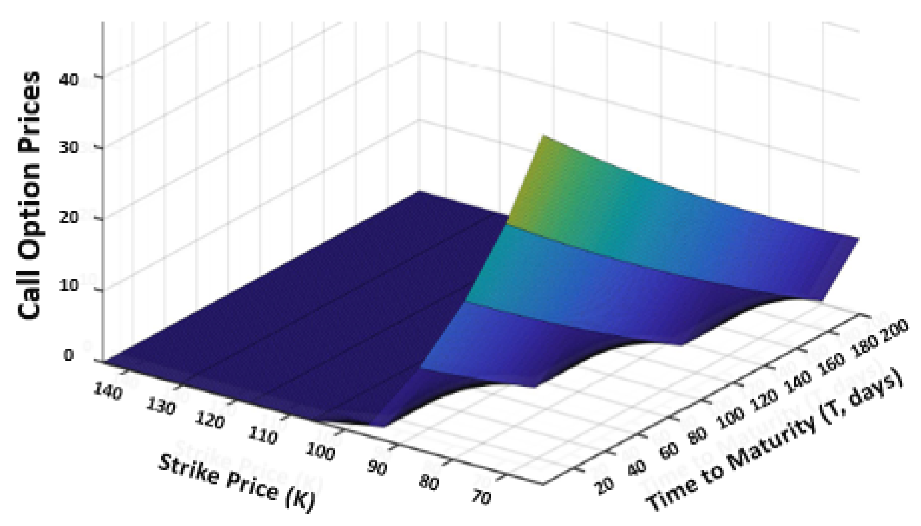
In this section, we calculate the European call and put option prices for our portfolio using the pricing model, Equation (12), introduced in Section 3.1. We provide European option prices by fixing to 100 in Equation (12), i.e., the price of the crime portfolio at time zero is 100 units, and the time to maturity is in days. Later, we provide the implied volatilities of the portfolio based on the volatilities of call and put option prices.
First, we demonstrate the relationship between call option prices, strike price, and time to maturity in Figure 1. These calculated prices help the investors to strategize buying the stocks in our portfolio at a predefined price within a specific time frame . Second, we show put option prices in Figure 2 to provide selling prices of the shares in our index. The prices of our options validate the fact that option prices decrease as the time to maturity increases for a given strike price.
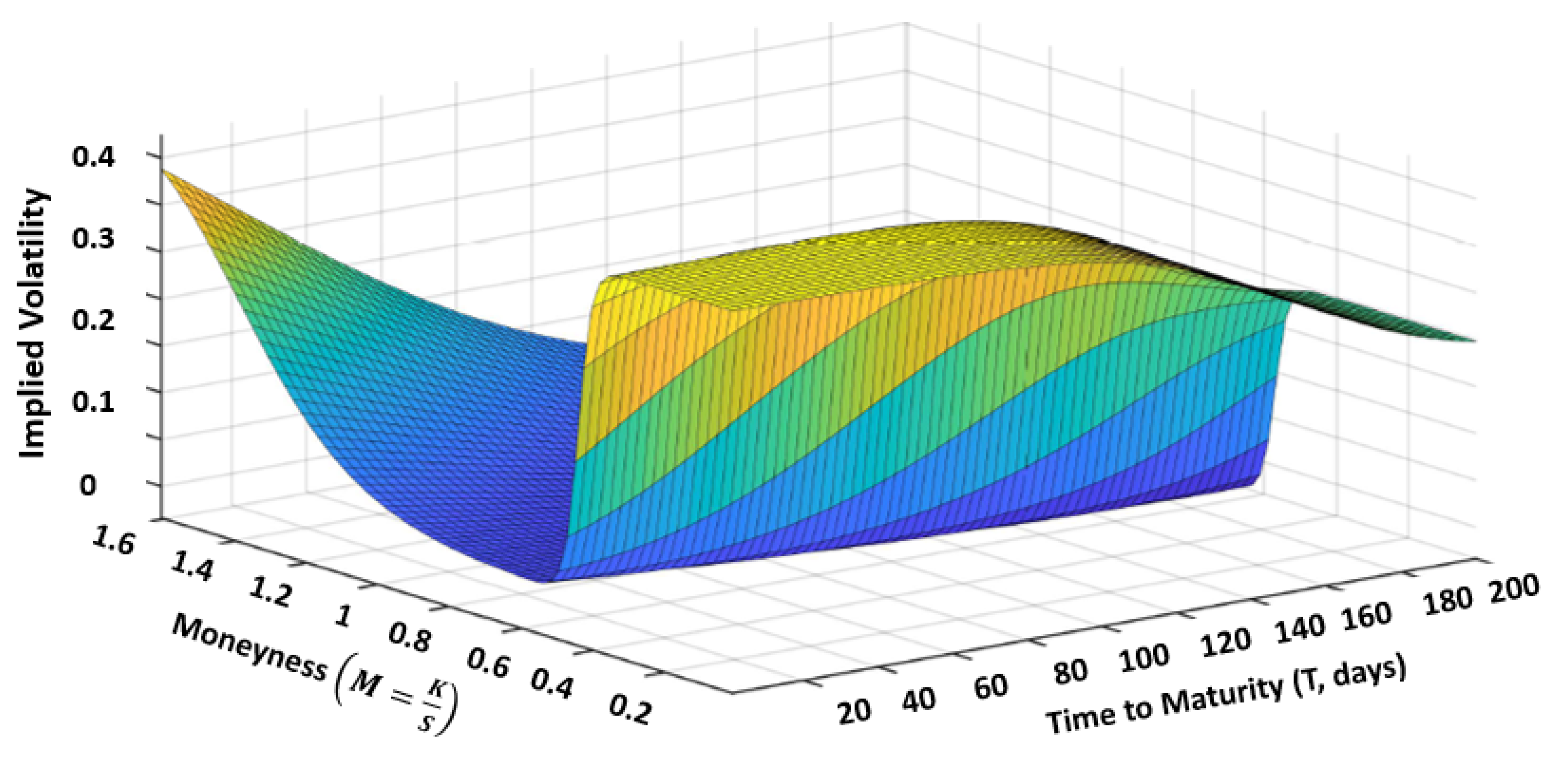
Third, we determine the implied volatilities of our portfolio using the Black–Scholes and Merton model. This provides the expected volatility of our portfolio over the life of the option . Figure 3 is the implied volatility surface with respect to moneyness (M) and time to maturity (T). In particular, we calculate moneyness as the strike price over the stock price, i.e., . Then, the volatilities for call and put option prices are shown in the regions of the surface with and , respectively. The volatility surface demonstrates a volatility smile, which is usually seen in the stock market.
Figure 3 illustrates that implied volatility increases when the moneyness is further out of the money or in the money, compared to at the money . In this case, volatility seems to be low, with a range of 0.8 and 1.2 in moneyness, compared to the other regions in the implied volatility surface, i.e., the options with higher premiums result in high implied volatilities. These findings help investors strategize buying call options and selling put options in our portfolio based on their desired risk level and predicted volatilities.
4. Risk Budgets for the Crime Portfolio
The investors intend to optimize portfolio performance while maintaining their desired risk tolerance level (Mahanama and Shirvani 2020). In this section, we provide a rationale for investors to determine the degree of variability in our portfolio. Therefore, we provide the risk contribution related to each type of crime in Section 4.2 using the risk measures defined in Section 4.1. As a result, we present the main risk contributors and risk diversifiers in our portfolio. Ultimately, these risk budgets (the estimated risk allocations) will potentially help investors with their financial planning (maximizing the returns).
4.1. Defining Tail and Center Risk Measures
This section defines the risk measures that we use for assessing risk allocations in Section 4.2. We determine the tail risk contributors and center risk contributors using expected tail loss and volatility risk measures, respectively (Boudt et al. 2013; Chow and Kritzman 2001).
We use Conditional Value at Risk (CoVaR) (Adrian and Brunnermeier 2011; Girardi and Ergun 2013) for finding the tail risk contributors in our portfolio at levels of 95% and 99%. We define the tail risk contribution of the ith asset at level as follows:
In order to find center risk contributors, we measure the volatility of asset prices using standard deviation. Since we utilize an equally-weighted portfolio, we denote the weight vector for 32 types of crimes as where . We define the volatility risk measure, , using the covariance matrix, , of asset returns (Hu et al. 2019):
Then, the center risk contribution of the ith asset is given by
Having outlined the risk measures, Section 4.2 utilizes tail and center risk contributions to find the risk allocation for each type of crime defined in Section 2.1.
4.2. Determining the Risk Budgets for the Crime Portfolio
This section assesses the risk attributed to each type of crime using the risk measures defined in Section 4.1. First, we calculate the tail risk allocations () using Equation (13) to find the main tail risk contributors in our portfolio. Then, we investigate the main center risk contributors in our index using center risk allocations () computed using Equation (15). Finally, taking the main tail risk and center risk contributors into account, we find the main risk contributors of our portfolio.
In Table 4, we provide the center risk () and tail risk () allocations for each type of crime. We find the risk diversifiers in the portfolio using the negative risk allocations shown in Table 4. With significantly low center and tail risk diversifications, misrepresentation and social media seem to be the potential main risk diversifiers in our portfolio.
We consider the positive values outlined in Table 4 to identify the main risk contributors in our portfolio. We find the main tail risk contributors using the positive tail risk estimates at levels of 95% and 99%. At the 95% level, real estate, ransomware, and government impersonation provide a relatively higher tail risk than the other factors. However, real estate, ransomware, and identity theft seem to be the main tail risk contributors at the 99% level, .
We determine the main center risk contributors in our portfolio using the positive center risk estimates, , illustrated in Table 4. Since real estate, ransomware, and government impersonation demonstrate high volatility compared to the other types of crimes, they seem to be the main center risk contributors in our portfolio.
As real estate and ransomware are both main tail risk and center risk contributors, they are the potential main risk contributors. These estimated risk budgets and the main risk contributors will help investors to envision the amount of risk exposure with financial planning in our portfolio.
5. Performance of the Crime Portfolio for Economic Crisis
We evaluate the performance of our portfolio using economic factors related to low income as they are known to be major root causes of crime. To investigate the robustness of the crime portfolio for inevitable economic crashes, we perform stress testing in Section 5.2 based on the systemic risk measures defined in Section 5.1 The findings of this section are intended to help to determine portfolio risks and serve as a tool for hedging strategies required to mitigate inevitable economic crashes.
5.1. Defining Systemic Risk Measures
In this section, we define the systemic risk measures used for stress testing the portfolio on crimes. We define three derived risk measures based on VaR, Equation (5), denoting Y as the portfolio and X as a stress factor (Trindade et al. 2020).
CoVaR is a coherent measure of tail risk in an investment portfolio. In our study, we use a variant of CoVaR defined in terms of copulas (Mainik and Schaanning 2014). Using the condition rather than the traditional CoVaR condition, , improves the response to dependence between X and Y. We define CoVaR at level as
The CoVaR for the closely associated expected shortfall is defined as the tail mean beyond VaR (Mainik and Schaanning 2014). Furthermore, we use an extension of CoVaR denoted as Conditional Expected Shortfall (CoES). Then, we define CoES at level as follows:
Conditional Expected Tail Loss (CoETL) (Biglova et al. 2014) is the average of the portfolio losses when all the assets are in distress. CoETL is an appropriate risk measure to quantify the portfolio downside risk in the presence of systemic risk. We denote CoETL at level as
We quantify the market risk of our portfolio on crime using these systemic risk measures in Section 5.2.
5.2. Evaluating the Performance of the Crime Portfolio for Economic Factors
In this section, we evaluate how well our portfolio would perform with economic factors related to low income. In particular, we test the impact of the unemployment rate, poverty rate, and median household income on our index. We quantify the potential impact of these economic factors on our index using the systemic risk measures defined in Section 5.1. Since the stress testing results indicate the investment risk in our portfolio, the investors can utilize the outcomes to hedge strategies for forthcoming economic crashes.
Based on backtesting results in Section 2.3, we use the ARMA(1,1)-GARCH(1,1) model with Student’s t innovations for the log returns of our portfolio. In addition, we apply this filter to log returns of the economic factors to eliminate inherent linear and nonlinear dependencies. Then, we fit bivariate NIG models to the joint distributions of independent and identically distributed standardized residuals of each economic factor and our portfolio on crime. Using these bivariate models, we generate 10,000 simulations for each joint density to perform a scenario analysis. In Table 5, we provide the empirical correlation coefficients of each simulated joint density with the corresponding economic factor. This table demonstrates weak correlations between the economic factors and the portfolio.
We utilize the simulated joint densities to compute the systemic risk measures. In Table 6, we provide the left tail systemic risk measures (CoVaR, CoES, and CoETL) on the portfolio at stress levels of 10%, 5%, and 1% on the economic factors - unemployment rate, poverty rate, and household income. At each level, the unemployment rate provides the highest values for the three systemic risk measures compared to the other economic factors. Thus, among all the stressors, the unemployment rate demonstrates a significantly high impact on the index. The poverty rate potentially has a low impact on the index according to the results of all three systemic risk measures at all stress levels. Our key findings are consistent with the studies outlined in Section 1 on examining the effects of unemployment and poverty indicators on crime rate (Lieberman and Smith 1986; Raphael and Winter-Ebmer 2001; Wadsworth 2001). In addition, we compare the effects of these economic factors on our crime index.
In conclusion, the unemployment rate potentially has a high impact on the financial losses due to crimes in the United States. Hence, these findings will help portfolio managers gauge the market risk of our index to alleviate potential losses due to economic crashes by hedging strategies such as utilizing options, risk budgets, and transferring risk to capital market investors.
6. Discussion and Conclusions
We proposed constructing a portfolio that outlines the financial impacts of various types of crimes in the United States. In order to do that, we modeled the financial losses of crimes reported by the Federal Bureau of Investigation using the annual cumulative property losses caused by property crimes and cybercrimes. Then, we backtested the index using VaR models at different levels to find a proper model for implementing in evaluation processes. As a result, we utilized ARMA(1,1)-GARCH(1,1) with the Student’s t model to evaluate the crime portfolio.
We presented the use of our portfolio on crimes through option pricing, risk budgeting, and stress testing. First, we provided fair values for European call and put option prices and implied volatilities for our portfolio. Second, we found the risk attributed to each type of crime based on tail risk and center risk measures. Third, we evaluated the performance of our index for the economic crisis by implementing stress testing. According to the findings, in the United States, the unemployment rate potentially has a higher impact on the financial losses due to the crimes incorporated in this study compared to the poverty rate and median household income.
The proposed portfolio on crimes is an attempt to implement a financial instrument for hedging the intrinsic risk induced by crime in the United States. The goal of our paper is to introduce new risk hedging financial contracts for crime, consistent with dynamic asset pricing to forecast the degree of future systemic risk. The findings, estimated option prices, risk budgets, and systemic risk outlined in the portfolio will help investors with financial planning and forewarn them to transfer insurance risk to capital market investors. While the portfolio on crimes is specifically constructed for the United States, it could be modified to calculate the risk in other regions or countries using a data set comparable to the FBI’s reported crime data.
Author Contributions
Conceptualization, methodology, supervision, project administration, S.T.R.; software, writing—original draft preparation, T.M. and A.S.; data curation, T.M.; investigation, visualization, formal analysis, writing—review and editing, T.M., A.S. and S.T.R. All authors have read and agreed to the published version of the manuscript.
Funding
This research received no external funding.
Institutional Review Board Statement
Not applicable.
Informed Consent Statement
Not applicable.
Data Availability Statement
The reported financial losses for property crimes in uniform crime reports and cybercrimes in internet crime reports published by the Federal Bureau of Investigation were used in this study.
Conflicts of Interest
The authors declare no conflict of interest.
| 1 | |
| 2 | See (Black and Scholes 1973) and (Merton 1973). |
| 3 |
References
- Adrian, Tobias, and Markus K. Brunnermeier. 2011. Covar; Technical Report. Cambridge: National Bureau of Economic Research.
- Anderson, Ross, Chris Barton, Rainer Böhme, Richard Clayton, Michel J. G. Van Eeten, Michael Levi, Tyler Moore, and Stefan Savage. 2013. Measuring the cost of cybercrime. In The Economics of Information Security and Privacy. New York: Springer, pp. 265–300. [Google Scholar]
- Barndorff-Nielsen, Ole E. 1997. Normal inverse gaussian distributions and stochastic volatility modelling. Scandinavian Journal of Statistics 24: 1–13. [Google Scholar] [CrossRef]
- Bell, Richard A. 2006. Option Pricing with the Extreme Value Distributions. London: University of London. [Google Scholar]
- Biglova, Almira, Sergio Ortobelli, and Frank J. Fabozzi. 2014. Portfolio selection in the presence of systemic risk. Journal of Asset Management 15: 285–99. [Google Scholar] [CrossRef]
- Black, Fischer, and Myron Scholes. 1973. The pricing of options and corporate liabilities. The Journal of Political Economy 81: 637–54. [Google Scholar] [CrossRef] [Green Version]
- Black, Fischer, and Myron Scholes. 2019. The pricing of options and corporate liabilities. In World Scientific Reference on Contingent Claims Analysis in Corporate Finance: Volume 1: Foundations of CCA and Equity Valuation. Singapore: World Scientific, pp. 3–21. [Google Scholar]
- Blumstein, Alfred. 1974. Seriousness weights in an index of crime. American Sociological Review 79: 854–64. [Google Scholar] [CrossRef]
- Bollerslev, Tim. 1986. Generalized autoregressive conditional heteroskedasticity. Journal of Econometrics 31: 307–27. [Google Scholar] [CrossRef] [Green Version]
- Boudt, Kris, Peter Carl, and Brian G. Peterson. 2013. Asset allocation with conditional value-at-risk budgets. Journal of Risk 15: 39–68. [Google Scholar] [CrossRef]
- Braione, Manuela, and Nicolas K. Scholtes. 2016. Forecasting value-at-risk under different distributional assumptions. Econometrics 4: 3. [Google Scholar] [CrossRef] [Green Version]
- Carr, Peter, and Dilip Madan. 1998. Option valuation using the fast fourier transform. Journal of Computational Finance 2: 61–73. [Google Scholar] [CrossRef] [Green Version]
- Carr, Peter, and Liuren Wu. 2004. Time-changed lévy processes and option pricing. Journal of Financial Economics 71: 113–41. [Google Scholar] [CrossRef] [Green Version]
- Chalfin, Aaron. 2015. Economic costs of crime. The Encyclopedia of Crime and Punishment, 1–12. [Google Scholar] [CrossRef]
- Chow, George, and Mark Kritzman. 2001. Risk budgets. Journal of Portfolio Management 27: 56–60. [Google Scholar] [CrossRef]
- Clark, Peter K. 1973. A subordinated stochastic process model with finite variance for speculative prices. Econometrica: Journal of the Econometric Society 41: 135–55. [Google Scholar] [CrossRef]
- Collins, Mark F. 1988. Some cautionary notes on the use of the sellin-wolfgang index of crime seriousness. Journal of Quantitative Criminology 4: 61–70. [Google Scholar] [CrossRef]
- Delbaen, Freddy, and Walter Schachermayer. 1994. A general version of the fundamental theorem of asset pricing. Mathematische annalen 300: 463–520. [Google Scholar] [CrossRef]
- Epperlein, Thomas, and Barbara C. Nienstedt. 1989. Reexamining the use of seriousness weights in an index of crime. Journal of Criminal Justice 17: 343–60. [Google Scholar] [CrossRef]
- Fama, Eugene F., and Kenneth R. French. 2015. A five-factor asset pricing model. Journal of Financial Economics 116: 1–22. [Google Scholar] [CrossRef] [Green Version]
- Girardi, Giulio, and A. Tolga Ergun. 2013. Systemic risk measurement: Multivariate garch estimation of coVaR. Journal of Banking & Finance 37: 3169–80. [Google Scholar]
- Hindelang, Michael J. 1974. The uniform crime reports revisited. Journal of Criminal Justice 2: 1–17. [Google Scholar] [CrossRef]
- Hu, Yuan, Svetlozar T. Rachev, and Frank J. Fabozzi. 2019. Modelling crypto asset price dynamics, optimal crypto portfolio, and crypto option valuation. arXiv arXiv:1908.05419. [Google Scholar]
- Hurst, Simon R., Eckhard Platen, and Svetlozar T. Rachev. 1997. Subordinated market index models: A comparison. Financial Engineering and the Japanese Markets 4: 97–124. [Google Scholar] [CrossRef]
- Hurst, Simon R., Eckhard Platen, and Svetlozar Todorov Rachev. 1999. Option pricing for a logstable asset price model. Mathematical and Computer Modelling 29: 105–19. [Google Scholar] [CrossRef]
- Internet Crime Complaint Center, Federal Bureau of Investigation. 2019. Crime in the United States. Available online: https://www.fbi.gov/news/pressrel/press-releases/fbi-releases-the-internet-crime-complaint-center-2019-internet-crime-report (accessed on 8 July 2021).
- Jorion, Philippe. 2007. Value at Risk: The New Benchmark for Managing Financial Risk. New York: McGraw-Hill Professional. [Google Scholar]
- Josse, Julie, Jérôme Pagès, and François Husson. 2011. Multiple imputation in principal component analysis. Advances in Data Analysis and Classification 5: 231–46. [Google Scholar] [CrossRef]
- Ken-Iti, Sato. 1999. Lévy Processes and Infinitely Divisible Distributions. Cambridge: Cambridge University Press. [Google Scholar]
- Klingler, Sven, Young Shin Kim, Svetlozar T. Rachev, and Frank J. Fabozzi. 2013. Option pricing with time-changed lévy processes. Applied Financial Economics 23: 1231–38. [Google Scholar] [CrossRef] [Green Version]
- Kwan, Ying Keung, Wai Cheung Ip, and Patrick Kwan. 2000. A crime index with thurstone’s scaling of crime severity. Journal of Criminal Justice 28: 237–44. [Google Scholar] [CrossRef]
- Lieberman, Louis, and Alexander B. Smith. 1986. Crime rates and poverty—A reexamination. Crime and Social Justice, 166–77. [Google Scholar]
- Lugo, Kristina, Roger Przybylski, Justice Research, Statistics Association, and United States of America. 2019. Estimating the Financial Costs of Crime Victimization. Washington, DC: National Criminal Justice Reference Service. [Google Scholar]
- Madan, Dilip B., Frank Milne, and Hersh Shefrin. 1989. The multinomial option pricing model and its brownian and poisson limits. The Review of Financial Studies 2: 251–65. [Google Scholar] [CrossRef]
- Mahanama, Thilini V., and Abootaleb Shirvani. 2020. A natural disasters index. arXiv arXiv:2008.03672. [Google Scholar]
- Mainik, Georg, and Eric Schaanning. 2014. On dependence consistency of covar and some other systemic risk measures. Statistics & Risk Modeling 31: 49–77. [Google Scholar]
- Mandelbrot, Benoit, and Howard M. Taylor. 1967. On the distribution of stock price differences. Operations Research 15: 1057–62. [Google Scholar] [CrossRef]
- Maure, Diana. 2017. Costs of Crime: Experts Report Challenges Estimating Costs and Suggest Improvements to Better Inform Policy Decisions. Available online: https://www.gao.gov/products/gao-17-732 (accessed on 8 July 2021).
- McCollister, Kathryn E., Michael T. French, and Hai Fang. 2010. The cost of crime to society: New crime-specific estimates for policy and program evaluation. Drug and Alcohol Dependence 108: 98–109. [Google Scholar] [CrossRef] [Green Version]
- Merton, Robert C. 1973. Theory of rational option pricing. The Bell Journal of Economics and Management 4: 141–83. [Google Scholar] [CrossRef] [Green Version]
- Nieppola, Olli. 2009. Backtesting Value-at-Risk Models. Available online: https://aaltodoc.aalto.fi/handle/123456789/181 (accessed on 8 July 2021).
- Rachev, Svetlozar, Frank J. Fabozzi, Boryana Racheva-Iotova, and Abootaleb Shirvani. 2017. Option pricing with greed and fear factor: The rational finance approach. arXiv arXiv:1709.08134. [Google Scholar]
- Raphael, Steven, and Rudolf Winter-Ebmer. 2001. Identifying the effect of unemployment on crime. The Journal of Law and Economics 44: 259–83. [Google Scholar] [CrossRef] [Green Version]
- Robison, Sophia M. 1966. A critical view of the uniform crime reports. Michigan Law Review 64: 1031–54. [Google Scholar] [CrossRef]
- Shirvani, Abootaleb, Frank J. Fabozzi, and Stoyan V. Stoyanov. 2020. Option pricing in an investment risk-return setting. arXiv arXiv:2001.00737. [Google Scholar]
- Shirvani, Abootaleb, Svetlozar T. Rachev, and Frank J. Fabozzi. 2020. Multiple subordinated modeling of asset returns: Implications for option pricing. Econometric Reviews 40: 290–319. [Google Scholar] [CrossRef]
- Trindade, A. Alexandre, Abootaleb Shirvani, and Xiaohan Ma. 2020. A socioeconomic well-being index. arXiv arXiv:2001.01036. [Google Scholar] [CrossRef]
- United States Department of Justice, Federal Bureau of Investigation. 2011. Crime in the United States. Available online: https://ucr.fbi.gov/crime-in-the-u.s/2011 (accessed on 8 July 2021).
- United States Department of Justice, Federal Bureau of Investigation. 2019. Crime in the United States. Available online: https://ucr.fbi.gov/crime-in-the-u.s/2019 (accessed on 8 July 2021).
- Wadsworth, Thomas P. 2001. Employment, Crime, and Context: A Multi-Level Analysis of the Relationship between Work and Crime. Washington, DC: University of Washington. [Google Scholar]
- Weissman, Michael L. 2017. Banker’s fidelity bond did not cover losses because it terminated due to earlier employee dishonesty. The RMA Journal 99: 63. [Google Scholar]
- Whittle, Peter. 1953. The analysis of multiple stationary time series. Journal of the Royal Statistical Society: Series B (Methodological) 15: 125–39. [Google Scholar] [CrossRef]
Figure 1.
Call option prices against time to maturity (T, in days) and strike price (K, based on ).

Figure 2.
Put option prices against time to maturity (T, in days) and strike price (K, based on ).

Figure 3.
Implied volatility surface against time to maturity (T, in days) and moneyness (, the ratio of strike price, K, and stock price, S).
Figure 3.
Implied volatility surface against time to maturity (T, in days) and moneyness (, the ratio of strike price, K, and stock price, S).


Table 1.
VaR Backtesting Results for ARMA(1,1)-GARCH(1,1) with Student’s t and NIG innovations.
| Innovation | VaR Level | Test Results | |||
|---|---|---|---|---|---|
| Traffic Light | Binomial | PoF | CCI | ||
| Student’s t | 0.01 | green | reject | reject | accept |
| 0.05 | green | accept | accept | accept | |
| 0.25 | green | reject | reject | accept | |
| 0.50 | green | accept | accept | accept | |
| 0.75 | green | accept | accept | accept | |
| 0.95 | green | accept | accept | accept | |
| 0.99 | yellow | accept | accept | accept | |
| NIG | 0.01 | green | reject | reject | accept |
| 0.05 | green | reject | reject | accept | |
| 0.25 | green | reject | reject | accept | |
| 0.50 | green | accept | accept | accept | |
| 0.75 | yellow | reject | reject | accept | |
| 0.95 | red | reject | reject | accept | |
| 0.99 | red | reject | reject | accept | |
Table 2.
The estimated parameters of the fitted ARMA(1,1)-GARCH(1,1) with Student’s t innovations to the crime portfolio log returns.
Table 2.
The estimated parameters of the fitted ARMA(1,1)-GARCH(1,1) with Student’s t innovations to the crime portfolio log returns.
| Parameters | |||||
|---|---|---|---|---|---|
| Estimates | −0.0005 | 0.1655 | −0.0827 | 0.0233 | 1.0000 |
Table 3.
The estimated parameters of the fitted the NIG process to the crime portfolio log returns.
| Parameters | ||||
|---|---|---|---|---|
| Estimates | −0.0014 | 0.4826 | 0.0006 | 0.6553 |
Table 4.
The percentages of center risk (CR) and tail risk (TR) (at levels of 95% and 99%) budgets for the portfolio on crimes.
Table 4.
The percentages of center risk (CR) and tail risk (TR) (at levels of 95% and 99%) budgets for the portfolio on crimes.
| Crime Type | (95) | (99) | |
|---|---|---|---|
| Real Estate | 13.62 | 12.93 | 11.29 |
| Ransomware | 10.35 | 11.40 | 8.48 |
| Government Impersonation | 9.48 | 8.80 | 8.25 |
| Identity Theft | 7.96 | 10.23 | 6.74 |
| Extortion | 7.72 | 6.90 | 7.19 |
| Lottery | 7.09 | 7.37 | 6.26 |
| Confidence Fraud | 5.56 | 6.64 | 5.48 |
| Investment | 5.31 | 7.11 | 4.90 |
| Crimes Against Children | 5.24 | 3.95 | 5.55 |
| Personal Data Breach | 3.69 | 4.29 | 3.24 |
| Credit Card Fraud | 3.58 | 3.16 | 3.96 |
| BEC/EAC | 3.27 | 3.29 | 3.00 |
| Non−Payment | 2.56 | 4.38 | 2.10 |
| IPR Copyright | 2.02 | 2.04 | 1.95 |
| Gambling | 1.97 | 2.55 | 1.40 |
| Robbery | 1.80 | 0.67 | 6.77 |
| Phishing | 1.48 | 0.97 | 2.01 |
| Civil Matter | 1.30 | −0.57 | 2.89 |
| Denial Of Service | 1.02 | −0.23 | 2.74 |
| Motor Vehicle Theft | 1.01 | 1.30 | 0.73 |
| Check Fraud | 0.98 | 2.19 | −0.51 |
| Advanced Fee | 0.75 | 0.43 | 1.04 |
| Harassment | 0.74 | 0.10 | 1.14 |
| Corporate Data Breach | 0.70 | 0.03 | 0.90 |
| Larceny Theft | 0.50 | 0.56 | 0.39 |
| Terrorism | 0.36 | −0.20 | 2.06 |
| Burglary | 0.30 | 0.21 | 0.44 |
| Employment | 0.22 | 0.09 | 0.29 |
| Charity | 0.17 | 0.18 | 0.54 |
| Overpayment | −0.04 | −0.23 | 0.10 |
| Social Media | −0.16 | −0.17 | −0.31 |
| Misrepresentation | −0.55 | −0.41 | −1.00 |
Table 5.
The empirical correlation coefficients of the joint densities of each economic factor and the crime portfolio.
Table 5.
The empirical correlation coefficients of the joint densities of each economic factor and the crime portfolio.
| Economic Factor | Correlation Coefficient |
|---|---|
| Unemployment Rate | 0.11 |
| Poverty Rate | −0.24 |
| Household Income | 0.17 |
Table 6.
The left tail systemic risk measures (CoVaR, CoES, and CoETL) on the portfolio at stress levels of 10%, 5%, and 1% on the following economic factors—unemployment rate, poverty rate, and Household Income.
Table 6.
The left tail systemic risk measures (CoVaR, CoES, and CoETL) on the portfolio at stress levels of 10%, 5%, and 1% on the following economic factors—unemployment rate, poverty rate, and Household Income.
| Economic Factors | Stress Levels | Left Tail Risk Measures | ||
|---|---|---|---|---|
| CoVaR | CoES | CoETL | ||
| Unemployment Rate | 10% | −5.88 | −8.85 | −5.23 |
| 5% | −9.01 | −12.27 | −7.06 | |
| 1% | −14.82 | −16.32 | −11.50 | |
| Poverty Rate | 10% | −0.67 | −1.29 | −0.92 |
| 5% | −1.31 | −2.07 | −1.24 | |
| 1% | −2.42 | −3.15 | −2.05 | |
| Household Income | 10% | −1.45 | −2.14 | −1.20 |
| 5% | −2.30 | −2.91 | −1.66 | |
| 1% | −3.71 | −3.86 | −2.46 | |
Publisher’s Note: MDPI stays neutral with regard to jurisdictional claims in published maps and institutional affiliations. |
© 2021 by the authors. Licensee MDPI, Basel, Switzerland. This article is an open access article distributed under the terms and conditions of the Creative Commons Attribution (CC BY) license (https://creativecommons.org/licenses/by/4.0/).
Share and Cite
MDPI and ACS Style
Mahanama, T.; Shirvani, A.; Rachev, S.T. Global Index on Financial Losses Due to Crime in the United States. J. Risk Financial Manag. 2021, 14, 315. https://0-doi-org.brum.beds.ac.uk/10.3390/jrfm14070315
AMA Style
Mahanama T, Shirvani A, Rachev ST. Global Index on Financial Losses Due to Crime in the United States. Journal of Risk and Financial Management. 2021; 14(7):315. https://0-doi-org.brum.beds.ac.uk/10.3390/jrfm14070315
Chicago/Turabian StyleMahanama, Thilini, Abootaleb Shirvani, and Svetlozar T. Rachev. 2021. "Global Index on Financial Losses Due to Crime in the United States" Journal of Risk and Financial Management 14, no. 7: 315. https://0-doi-org.brum.beds.ac.uk/10.3390/jrfm14070315