What Information in Financial Statements Could Be Used to Predict the Risk of Equity Investment?

Abstract

Theoretically, accounting earnings could be used to estimate the intrinsic value of equity. If accounting earnings could be predicted accurately, then, so could be the value of equity, thereby, creating much less risk in equity investment. However, earnings surprises are common, and therefore so is the risk in equity investment. To quantify the risk in the investment implied from accounting earnings, I propose to use financial statements to construct abnormal sales growth rates (ABG) and abnormal changes in profit margins (ABPM) to measure the uncertainty embedded in the accounting earnings. I measure ABG (ABPM) as the difference between the current value of sales growth rate (profit margin) and its benchmark, a weighted value of the three preceding years’ sales growth rate (profit margin). Then, I quantify whether and to what extent the news of ABG and ABPM are material enough to change the expected earnings (proxied by analysts’ forecasted earnings revisions [FREV] and predicted unexpected earnings [UE], and future stock returns [SAR]). Fama–MacBeth regression results show that, together, solely ABPM and ABG could explain 8.2% (2.3%) (5.4%) of the variation of FREV (UE) (SAR). The risk-predictability of ABPM and ABG is robust to the presence of abnormal growth in net operating assets and accruals quality, which, suggested by previous literature, might influence unexpected earnings. Further contingent analyses indicate that the capital market reacts more strongly to the bad news embedded in the ABPM/ABG (with negative signs) than the good news in ABPM/ABG (with positive signs).

1. Introduction

Sell-side security analysts primarily provide future earnings forecasts and stock recommendations. Prior studies provide empirical evidence that changes in expectations of future earnings (forecast revisions) will result in changes in stock prices because of the role that earnings play in valuation (e.g., Barth and Hutton 2004; Gleason and Lee 2003; Stickel 1991). This paper examines which unexpected future earnings indicators, obtained from financial statements, lead to forecast revisions.

Financial analysts usually break down earnings into operating earnings and earnings from financial activities when forecasting future earnings. Forecasting operating earnings is the more challenging task for analysts. This paper focuses on the unexpected earnings drivers that cause changes in operating earnings. Earnings could be computed as the product of sales and profit margin. Therefore, in earnings forecasting, analysts usually begin with sales growth and operating profit margins obtained from firms’ financial statements. In this study, net operating assets growth is also considered, because the changes in current net operating assets might affect the firm’s profits in the next period. Consequently, when analysts forecast future earnings, they may compute the net operating assets growth, measured by how much capital retained from current period earnings to reinvest into the next operating period. Further, to figure out whether these financial indicators are reliable, analysts investigate the reported earnings quality to find out whether current earnings are good predictors for future earnings. Thus, I examine whether these three financial items contain any useful information to predict future earnings, and whether analysts factor in earnings quality in earnings forecasts.

The proxies for unexpected earnings predictors are measured by the differences between the actual values of three items and their benchmarks. First, the benchmark (or expected value) of each unexpected earnings indicator is measured as a weighted value of the prior three years’ values of each given variable (the weights are chosen as 0.4, 0.3, and 0.3 for years t − 1, t − 2, and t − 3 respectively).1 Then, abnormal sales growth (ABG), abnormal changes in operating profit margins (ABPM), and abnormal growth in net operating assets (ABNOAG) are computed by subtracting the benchmark value of each unexpected earnings indicator variable from its current value. By doing so, each earnings surprise indicator not only reflects the change in the value of each variable, but also controls for the normal (or expected) value of each variable.

The profit margin indicates the firm’s ability to generate profits controlling for the costs matched with the revenues. A change in the profit margin reflects the change in the firm’s ability to generate profits, holding other factors constant and should, thereby, be useful to predict future earnings. A change in sales growth indicates a change in revenue growth and should, therefore, provide information to forecast future earnings. Therefore, if analysts regard a jump in profit margins in current period as a signal of possible increase in future profits, they might revise their earlier earnings forecast upward if the earlier one was too pessimistic. Similar analyses apply to abnormal sales growth.

As discussed above, analysts look at unexpected profitability indicators (ABPM and ABG) of a firm when they forecast future earnings. However, if firms do not increase their operating capital for future operation, then current period earnings might not be sustainable in the future because of the decline in operating assets used to generate future earnings. Therefore, analysts might also reference the changes in net operating assets (NOA) when they forecast future earnings (e.g., Penman 2009). Increased investments in operating assets in the current period might provide the firm more opportunities to engage in profitable projects in the future. Therefore, an increased NOA growth implies, possibly, increasing future earnings. If analysts perceive the increased investment in operating assets in the current period as good news for future earnings, they possibly revise forecasted earnings upward if they observe an upward abnormal growth in net operating assets.

However, if the current period earnings are not good indicators for future earnings then it will be difficult for analysts to forecast future earnings using current financial data. Penman and Zhang (2002a) suggest that earnings having good quality are good predictors of future earnings. Hence, analysts factor in firms’ earnings quality proxied by accruals quality when they revise earnings forecasts.2 The accruals quality is measured by a modified Jones (1991) cross-sectional industry adjusted total accruals. As well documented in the literature, the accruals components of the earnings are less persistent and means revert more quickly than the cash component of the earnings. Therefore, the current earnings with poor accruals quality are poor indicators for future earnings. Thus, analysts should discount the firm’s future earnings when they use current earnings with low accruals quality to predict future earnings.

Results from the Fama–MacBeth regression procedure are consistent with the above expectations. Unexpected earnings factors (ABG and ABPM) determine the changes in expectations of future earnings; analysts regard the abnormal growth in net operating assets (NOA) as a positive sign for future earnings; and analysts revise downward forecasted earnings for firms with poor accruals quality. Results of the forecast revision regression show that the forecast revisions are positively associated with abnormal changes in profit margins (ABPM), abnormal sales growth (ABG), abnormal growth in net operating assets (ABNOAG), and earnings quality (AQ). To convene my analyses, I would call ABPM, ABG, ABNOAG, and AQ unexpected earnings indictors. Moreover, consistent with traditional wisdom, analysts learn from their own mistakes and adjust their earnings forecasts by updating the information in their forecast errors made in the previous period. The results show that analysts change their forecasted earnings for the next period upward (or downward) if they observe that they were too pessimistic (or optimistic), measured as the forecast errors deflated by the prior period prices.

The finding that unexpected earnings indicators (ABG, ABPM, ABNOAG, and AQ) can explain the unexpected earnings in the unexpected earnings regression indicates that these unexpected earnings indicators at least could partially predict unexpected earnings. This result holds using different proxies for the unexpected earnings. This also suggests that the determinants of forecast revisions overlap to some extent with the determinants of unexpected earnings (or earnings surprise). These results imply that abnormal sales growth and abnormal changes in profit margins create earnings surprises, and analysts are able to catch some of these earnings surprises. While this paper might have omitted variables that researchers commonly face, the main analyses of the current paper concentrate on the impact of financial reporting information on the changes in expectations of future earnings. For the sake of these analyses’ being straightforward, I do not discuss other factors’ effects on the forecast revision documented in the literature.3 I acknowledge this limitation.

Finally, one might wonder whether these surprise indicators have any predictability for future returns. The regression of one-year-ahead size-decile-adjusted returns on these surprise factors shows that abnormal profit margins and earnings quality have explanatory power for future returns.

To further investigate the detailed effects of each surprise indicator on each outcome (forecast revisions [FREV], unexpected earnings [UE], and returns [SAR]), contingent table analyses are employed. Eleven two-by-two contingent tables are constructed based on either the positive or negative sign of each unexpected earnings indicator (ABPM, ABG, and ABNOAG) and each outcome variable (FREV, UE, and SAR)4. Results show that the matching between the (positive or negative) sign of each outcome variable (FREV, UE, and SAR), with contingence upon the same sign of the abnormal changes in profit margins variable (ABPM), is the best among all pairs of outcome variables and surprise indicators (ABG, ABPM, ABNOAG). I interpret this result as that profit margin surprise creates current period earnings surprise, that analysts weight the effect of ABPM most when they revise their earnings forecasts, and that the future size-adjusted returns agree more with the abnormal change in the profit margins than other surprise factors.

In sum, results in this paper suggest that abnormal sales growth, abnormal changes in operating profit margin, abnormal net operating assets growth, and earnings quality contain useful information to predict future earnings and returns, suggesting that fundamental analyses of financial reports are useful to outside investors. Thus, the results of the current paper indicate that firms could use financial statements to communicate with outsiders about their business operations, and investors could make informed investment decisions based on their analyses on financial indicators.

This study is different from recent relevant studies. Cheng et al. (2020) use analysts forecast earnings and sales to examine and find that analysts’ earnings and sales forecasts are generally optimistic, relatively more accurate than their benchmark models (modified random walk models) and contain serial correlation of forecast errors. Cheng et al. (2020) focus on the forecast properties of earnings and sales, while the current study focuses on the effect of unexpected information embedded in profit margins and sales growth obtained from financial statements on the change in the earnings forecasts, unexpected earnings, and future returns. Although Liu (2021) adopts the measurement of abnormal sales growth in this study, Liu (2021) has a different research focus from this study. Liu (2021) examines and finds that abnormal sales growth is positively associated with the information risk of financial statements and abnormal portfolio returns formed by the ranks of abnormal sales growth in the prior fiscal year. Chu and Ohlson (2019) argue and find that year-to-year changes in operating liability and assets could predict next period earnings, with controlling for the current period earnings. This finding of Chu and Ohlson (2019) is conceptually consistent with the finding in this paper, that changes in net operating assets could predict change in the expected future earnings, although Chu and Ohlson (2019) use a different measurement of change in operating assets from this study. Findings in Chu and Ohlson (2019) and this study, about the effect of operating asset growth on the future earnings, support the conventional wisdom that financial statements are useful for equity investors.

The next section discusses the relevant literature and research motivation. Section 3 develops hypotheses. Section 4 presents the research design. Section 5 describes data and sample selection. Section 6 presents and explains the empirical results. Section 7 discusses adjustment of sales growth and possible future research, artificial intelligence, and machine learning, followed by the conclusion in Section 8.

2. Relevant Literature and Research Motivation

This paper is related to three streams of literature: analyst earnings forecasts, the relation between earnings and valuation, and earnings quality.

Numerous studies have documented what information affects analysts’ earnings forecasts. For example, Lev and Thiagarjan (1993) examined twelve fundamental-based earnings persistence indicators, derived from practitioner-oriented analyst literature, and increase the explanatory power of an earnings-returns regression. Denis et al. (1994) found that analyst forecast revisions following dividend changes are consistent with dividend changes, providing information about future cash flows rather than about investment opportunities. Previts et al. (1994) find that analysts place heavy weight on earnings-related information, disaggregate the information beyond the GAAP-based disaggregation found in annual reports, extract non-recurring items, and rely heavily on management for information beyond annual reports. Kasznik and Lev (1995) documented that analysts’ forecast revisions in response to disappointing earnings accompanied by warnings are significantly more negative than the responses to disappointing earnings unaccompanied by warnings, suggesting that warnings occurring before negative earnings surprise have more permanent implications for future earnings. Chu and Ohlson (2019) examine and document that asset and liability accruals influence analysts’ earnings forecasts: (1) liability accruals are more informative than asset accruals; (2) both liability and assets accruals forecast ROA (return on assets) well; and (3) both liability and assets accruals are more informative for small firms.

Moreover, contemporary literature examines the pricing effects of the forecast revisions. This line of research suggests that, the market responds to the earnings forecast revisions differently, combining with other forecast characteristics (i.e., forecast age, forecast accuracy, analysts’ aptitude and celebrity, and etc.) (e.g., Bonner et al. 2003; Gleason and Lee 2003; and Clement and Tse 2003, 2005).

In addition to the aforementioned literature on the association between forecasted earnings and equity price, a stream of literature discusses how the components of reported earnings could be used in the valuation framework (e.g., Yohn 2020). Feltham and Ohlson (1995) and Penman (2006) reason the important role of operating earnings in the equity valuation. Penman and Zhang (2002b) and Penman (2006) explicitly reason that profit margin, sales growth, and net operating assets growth should influence future earnings.

Two recent studies (i.e., Cheng et al. 2020; and Liu 2021) are close to this study. However, they are different from this study in terms of research method and research focus. Cheng et al. (2020) examine and document empirical evidence that four forecast performances are related (i.e., optimism, relative accuracy with respect to benchmark model forecasts, forecast suboptimality, and serial correlation of forecast errors) to the two components (i.e., sales and profit margin) of analysts’ earnings forecasts, while this study examines the effect of abnormal changes in the two components of the earnings on unexpected earnings and further on the value of equity. Liu (2021) argues that the measurement of abnormal sales growth employed in this paper is a risk proxy, which is positively correlated with beta and have a U-shaped relationship with monthly abnormal returns of portfolio (measured by Jensen’s alpha) sorted by the ranks of the abnormal sales growth in the previous year

Besides the effect of the aforementioned factors (e.g., profit margin, sales growth, net operating assets) on the forecasted earnings, previous literature also documents that earnings quality influences future earnings. For instance, Penman and Zhang (2002a) define earnings quality as the extent to which current earnings accurately predict future earnings. Following Penman and Zhang (2002a), I define good earnings quality as “sustainable earnings” that current earnings is a good predictor of future earnings. The earnings contain two components: cash and accruals.5 Previous empirical works (Sloan 1996; Xie 2001; and Francis et al. 2004, 2005) show that earnings with poor accruals quality are less persistent than earnings with good accruals quality. Therefore, the earnings with good accruals quality would be higher quality and are a more reliable indicator for future earnings than earnings with poor accruals quality. Thus, I use accruals quality as the proxy for earnings quality. One stream of studies argues that accruals anomaly is just a special case of earnings growth (e.g., Fairfield et al. 2003; Zhang 2007; and Penman and Yehuda 2009). This paper extends these studies by investigating how accruals quality affects analysts’ forecast revisions. Specifically, I examine whether and the extent to which analysts incorporate accruals quality into their forecast revision with the presence of the unexpected earnings indicators.

Because of the important valuation role of the predicted future earnings (Miller and Modigliani 1961; and Ohlson 1995), any new empirical evidence on indicators of predicted future earnings from financial reports would be not trivial. Therefore, this paper contributes to analysts’ forecasts and valuation literature.

3. Hypotheses Development

Penman (2006) and Fairfield and Yohn (2001) suggest that analysts often use current growth and profitability as a starting point to predict future earnings.6 Two popular proxies for growth and profitability are sales growth and operating profit margin respectively. Sales growth shows a firm’s ability to generate future revenues and is the clearest number, before deducting any expenses, to obtain net income. If the sales of a firm do not grow, the future profit of the firm would be unlikely to increase no matter how profitable the firm currently is. However, current sales growth might not be a good indicator of future sales growth, because the firm might have the same sales growth in the prior few years or might have a declined current sales growth. Therefore, a firm without positive unexpected sales growth might not have positive unexpected earnings (or residual earnings in the valuation framework).7 Thus, analysts might analyze both current and historical data of the firm when they predict future performance of the firm. Empirically, I call unexpected sales growth abnormal sales growth. The abnormal sales growth is measured by the difference between the current sales growth and a weighted value of the past sales growth in the prior three years, which is the expected-benchmark value of the current sales growth. If analysts consider a big jump (or a drop) in sales growth as a good (or a bad) signal of future earnings compared with its sales growth in the preceding three years, analysts might revise one-period-ahead earnings forecast ($FEP{S}_t^{t+1}$) upward (or downward) if the earnings forecasts for two periods ahead ($FEP{S}_{t-1}^{t+1}$) were too pessimistic (or optimistic) after current financial statements are released.

I choose the preceding three years data as the benchmark to compare with the current data for the following reasons. First, a length of three years contains a relatively long history of a firm’s past performance, thereby, providing reasonable comparison of current and past performance. Secondly, the three-years-investigated horizon is not too long to provide useful information to predict next period’s sales growth because of a firm’s possible rapid changes in business operations and economic environments.

The profit margin represents the operating efficiency. A positive change in the profit margin indicates the likelihood of increasing future earnings (i.e., profit), when holding sales constant. However, similar to the analyses for sales growth, analysts want to figure out whether the change in the profit margin is an indicator for predicting future earnings by counting into profit margins of the prior few years to mitigate its trend effect. In this study, I call unexpected change in profit margins abnormal changes in profit margins. If analysts regard the increased (or decreased) abnormal changes in the profit margins as a positive (or negative) signal for future earnings, they might revise their one-period-ahead earnings forecast ($FEP{S}_t^{t+1}$) upward (or downward) from two-periods-ahead earnings forecasts if they find out the two-periods-ahead earnings forecasts ($FEP{S}_{t-1}^{t+1}$) were too pessimistic (or optimistic) after current financial statements (at time t) are released.

After considering the two primary components of operating income, profit margin and sales (with adjusted growth), analysts would wonder whether the reported numbers they obtain from the financial statements are reliable in term of whether they are good indicators of future earnings. The literature suggests that accruals quality could be a proxy for the good/bad indicator of current earnings for future earnings (Francis et al. 2004, 2005). The better the accruals quality is; the better the earnings quality is. Therefore, analysts might revise downward (or upward) their one-year-ahead earnings forecast ($FEP{S}_t^{t+1}$) compared with forecasts made two years ahead ($FEP{S}_{t-1}^{t+1}$) after they find out if the firm’s accruals quality is bad (or good), compared with that of the firm’s industry peers.

Finally, analysts might count the growth of the net operating assets (NOA) that the firm has used to generate operating earnings. The increased net operating assets (NOA) reflect how much capital the firm retains from the current period adding to future NOA, which could be used to generate operating income. The increased NOA in the current period might increase the earnings in next period, holding other effects on the operating earnings constant. If analysts subtract the benchmark of NOAt growth for the current year (the average of the previous three years’ NOA growth) from the growth of NOA in the current year they would be able to determine whether a positive signal exists for NOAt growth. If this abnormal NOA growth is positive, then it could be a positive sign for the analyst who then would revise his previous earnings forecast upward. Thus, the first hypothesis is stated in the alternative form as follows:

Hypothesis 1 (H1).

The earnings forecast revisions are determined by abnormal profit margins, abnormal sales growth, abnormal change in net operating assets growth, and accruals quality.

Further, analysts revise their one-period-ahead earnings forecasts depending on whether their prior forecasts were too optimistic or pessimistic, usually proxied by forecast errors. Unexpected earnings are measured by the forecast errors deflated by the prior price. Then, one might wonder whether the same factors determining the forecast revisions will determine the unexpected earnings as well. Thus, the second hypothesis is stated in the alternative form as follow:

Hypothesis 2 (H2).

Unexpected earnings are determined by abnormal profit margins, abnormal sales growth, abnormal change in net operating assets growth, and accruals quality.

Ohlson (1995) suggests that the firm’s value is a function of the expected growth and earnings of the firm. Therefore, I would expect that the factors that determine the future earnings might be able to predict future returns, which are assumed to reflect the firm’s value. Thus, the third hypothesis is stated in the alternative form as follows:

Hypothesis 3 (H3).

Abnormal profit margins, abnormal sales growth, abnormal change in net operating assets growth, and accruals quality could predict future returns.

Then, the next section develops models used to test the above hypotheses.

4. Research Design

4.1. Model Used to Test H1

The following model in Equation (1) is a baseline model to test the first hypothesis discussed in Section 4.1. The subscript denotation for firm j is suppressed.

$$FRE{V}_{t-1,t}^{t+1}={\beta }_0+{\beta }_1{ABPM}_t+{\beta }_2{ABG}_t+{\beta }_3{AQ}_t+{\beta }_4{ABNOAG}_t+{\epsilon }_t$$

(1)

where, $FRE{V}_{t-1,t}^{t+1}$ is a forecast revision (a proxy for the change in expectations) of future earnings in period t, and this expected future earnings (t + 1) in period t compared with expectations for future earnings (t + 1) in period t − 1; the expectation of the future earnings (time t + 1) made at time t − 1 is estimated by the I/B/E/S consensus median (or mean)8 values of two-years-forward forecasted earnings per share ($FEP{S}_{t-1}^{t+1}$), and the expectation of the future earnings (time t + 1) made at t is estimated by the I/B/E/S consensus median (or mean) of the one-year-forward forecasted earnings per share ($FEP{S}_t^{t+1}$); and9

$$FRE{V}_{t-1,t}^{t+1}=(FEP{S}_t^{t+1}-FEP{S}_{t-1}^{t+1})/P_{t-1}.$$

ABPM_t denotes the abnormal profit margin in year t, measured as the operating profit margin (hereafter PM) in year t minus the benchmark value of PM of the firm j over the three preceding years.

$$\begin{array}{l}{\mathit{ABPM}}_t={\mathit{PM}}_t-{\mathit{PMBechmark}}_t\\ {\mathit{PMBechmark}}_t=0.3\times P{M}_{t-3}+0.3\times P{M}_{t-2}+0.4\times P{M}_{t-1}\end{array}$$

The profit margin (PM) is measured as the operating income (data#13, Operating Income before Depreciation) divided by sales (data#12). The operating income will increase with the increment of operating profit margin, holding sales consistent over time. This data item is the operating income before depreciation that includes the effects of adjustments for cost of goods sold and selling, general and administrative expenses, excluding effects of special items. Therefore, the income from operating is more persistent and might, thereby, have more predictive information for future earnings. The weighting scheme is arbitrarily chosen, basing on the assumption that the data of the most recent year is the most useful to predict future earnings, thereby, weight most heavily in this weighting scheme. In robustness tests, I change the weighting scheme by setting up the expected value of the PM as a moving average value of preceding three years data, the results of which are qualitatively similar to those using this weighting scheme. As discussed in the Section 3, if analysts regard an increased ABPM as a positive signal for predicted future earnings, then, the coefficient of the variable ABPM should be positive in the regression Equation (1) (β₁ > 0).

ABG_t denotes the abnormal sales growth in year t comparing with a benchmark value of sales growth of the firm itself over three preceding years.

$$\begin{array}{l}{\mathit{ABG}}_t={\mathit{SaleG}}_t-{\mathit{SalesGBechmark}}_t\\ {\mathit{SalesGBechmark}}_t=0.3\times Sales{G}_{t-3}+0.3\times Sales{G}_{t-2}+0.4\times Sales{G}_{t-1}\end{array}$$

where, SaleG_t is sales growth at year t, measured as the difference of sales (data#12) over time t − 1 and time t divided by sales in year t − 1 (∆Sales_t−1,t/Sales_t−1). SalesGBechmark_t is the benchmark sales growth at year t for a firm j, measured by a weighted value of the firm j’s sales growth in three preceding years. Similar to the weighting scheme of ABPM, in computing the abnormal sales growth and changes in profit margins, I assume that the later information is more value relevant to analysts when they compare the firm j’s performance in current year with firm j’s historical performance. Therefore, I arbitrarily assign a more weight (0.4) to sales growth in year t − 1 and an even weight (0.3) to the sales growth in year t − 2 and year t − 3. The abnormal sales growth is the difference between the sales growth in year t (SaleG_t) and the expected sales growth for year t, proxied by the benchmark sales growth over prior three years (SalesGBechmark_t). If analysts take an increased abnormal sales growth as a positive sign for predicted future earning, then, in year t, they might revise their earnings forecast for period t + 1 made in year t − t after the earnings announcement for year t is released. The coefficient of the ABG in the regression equation should be positive in the regression Equation (1) (β₂ > 0).

In Equation (1), I control for accrual quality (AQ_t) and the abnormal growth in net operating assets (ABNOAG_t), both of which might influence the outcome variables. I do not place ABNOAG_t before AQ_t in Equation (1), the same sequence as that I discussed the two control variable in previous Section 1 and Section 3, because I would like to keep the maximum observations that I could use to test my hypotheses. Please refer to the details of sample selection in Section 5.

AQ_t is the proxy for earnings quality in year t. It is difficult to measure unobservable earnings quality. I use the accruals quality as the proxy for the earnings quality, because of its popularity in current literature that suggests the current earnings with poor accruals quality are the poor predictor for future earnings. I measure the accruals quality as the industry adjusted AQ (Francis et al. 2005), using a modified Jones (1991) model mapping the current earnings to cash flows. (Please refer the appendix to the detailed measurement of the AQ variable). The larger value of the AQ indicates the poor accruals quality, thereby, poor earnings quality. If analysts discount the future earnings after they observe current reported earnings with poor accruals quality, then, in period t, they revise downward the forecasted earnings made two periods ahead (t − 1). Thus, the coefficient of AQ in should be negative in the regression Equation (1) (i.e., β₃ < 0). I use industry adjusted annual AQ because the industry AQ is a better benchmark for the firm, j, then that computed by the firm’s own data that requests at least ten years continuous data. Therefore, the way I have measured AQ in the current paper can avoid survivorship and provides comparing data of the firm with its industry peers.

ABNOAG_t is the proxy for the abnormal growth in net operating assets in year t comparing with a benchmark value of NOA growth of the firm itself over three preceding years.

$$\begin{array}{l}{\mathit{ABNOAG}}_t={\mathit{NOAG}}_t-{\mathit{NOAGBechmark}}_t\\ {\mathit{NOAGBechmark}}_t=0.3\times NOA{G}_{t-3}+0.3\times NOA{G}_{t-2}+0.4\times NOA{G}_{t-1}\end{array}$$

where, NOA is the net operating assets, measured as in (Fairfield et al. 2003). NOAG is the NOA growth (NOAG_t = ∆NOA_t−1,t /NOA_t−1). If analysts take an increased abnormal NOA growth as a positive sign for predicted future earnings, then, in year t, they might revise their earnings forecast for period t + 1 made in year t − t after earnings announcement for year t is released. The coefficient of the ABNOAG in the regression equation is expected to be positive in the regression Equation (1) (β₄ > 0). The detailed calculation of NOA is provided in the Appendix A.

As discussed in Section 3, analysts revise their earnings forecasts depending on whether they are too optimistic or pessimistic of their prior earnings forecasts. Therefore, the below Equation (2) adds the unexpected earnings as a control variable to Equation (1). If the information contained in four explanatory variables in Equation (1) is, at least partially, different from that in the unexpected earnings, then, I expect all these four independent variables to be still significant in the regression with the presence of the unexpected earnings.

$$FRE{V}_{t-1,t}^{t+1}={\beta }_0+{\beta }_1{\mathit{ABPM}}_t+{\beta }_2{\mathit{ABG}}_t+{\beta }_3{\mathit{AQ}}_t+{\beta }_4{\mathit{ABNOAG}}_t+{\beta }_5{\mathit{UE}}_t+{\nu }_t$$

(2)

Unexpected earnings (UE_t): measured as the difference between the actual earnings per share at time t (EPS_t) and the one-year-ahead median values of earnings forecasts reported in I/B/E/S at time t − 1 ($FEP{S}_{t-1}^t$), deflated by price per share at the beginning of the period (P_t−1).

$$U{E}_t=\frac{EP{S}_t-FEP{S}_{t-1}^t}{P_{t-1}}$$

(3)

Prior work has documented that the unexpected earnings is informative and value relevant. Therefore, if there is any earnings surprise during the periods from t − 1 and t, analysts might expect that there might be earnings surprise in next period from t to t + 1. Thus, I expect the coefficient of UE to be positive in the Equation (2) (β₅ > 0).

4.2. Model Used to Test H2

As discussed in Section 3, I expect that the set of explanatory variables for the forecast revision be able to explain the unexpected earnings; and, that the analyses for the regression of the unexpected earnings on the same set of independent variables are similar to those for the regression Equation (1). The signs of the coefficients in Equation (4) are expected to be the same as those in the Equation (1).

UE_t = γ₀ + γ₁ABG_t + γ₂ABPM_t + γ₃AQ_t + γ₄ABNOAG_t + δ_t

(4)

4.3. Model Used to Test H3

Similarly, the analyses for the one-year-ahead size-decile-adjusted return regression on the same set of the explanatory variables are applied to those for the forecast revision regression (Equation (1)). In Equation (6), the forecast revision variable is added into the baseline return model, Equation (5), as a control variable because of the value relevant role of the forecast revision in the literature.

SAR_j,_t = θ₀ + θ₁ABG_t + θ₂ABPM_t + θ₃AQ_t + θ₄ABNOAG_t + ξ_t

(5)

$${\mathit{SAR}}_{j,t}={\lambda }_0+{\lambda }_1{\mathit{ABG}}_t+{\lambda }_2{\mathit{ABPM}}_t+{\lambda }_3{\mathit{AQ}}_t+{\lambda }_4{\mathit{ABNOAG}}_t+{\lambda }_{5}FRE{V}_{t-1,t}^{t+1}+{\varsigma }_t$$

(6)

where, the SAR is the 12-months buy-and-hold size-adjusted returns (SAR), computed as below:

$$SA{R}_{j,t}=[\underset{t=1}{\overset{252}{{\displaystyle \mathsf{\Pi }}}}(1+R_{j,t})-\underset{t=1}{\overset{252}{{\displaystyle \mathsf{\Pi }}}}(1+R_{size,t})]-1$$

where R_j,t is firm j’s daily raw (cum dividend) return and R_size,t is the daily return of the size decile to which the firm j belongs as of the beginning of calendar year. Returns are cumulated beginning on the 1st day subsequent to the date of the last forecast revision reported in I/B/E/S before the earnings announcement. The one-year time horizon is selected because all variables used in this paper are based on annual data.

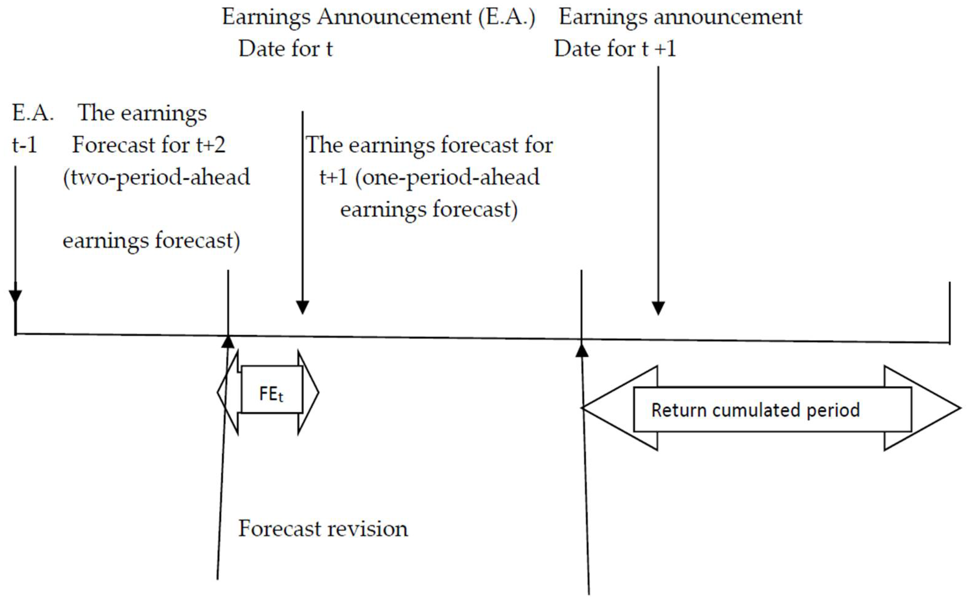
The Figure 1 illustrates the timeline of constructing variables in this section.

5. Sample Selection and Data

The sample selection involves multiple steps (shown as

Table 1. Sample Selection.

Descriptions	Firm-Year Observations	Distinct Firms
Firm-years listed on I/B/E/S, and Compustat databases from 1976 to 2006 (including all observations with available earnings forecasts data)	73,715	10,422
Less firm-years with
Missing Compustat data to compute abnormal   changes in profit margins and abnormal sales growth	10,232	1587
Initial sample	63,483	8835
Less firm-years with   Missing data to compute accruals quality   and excluding financial institutions firms	16,258	2342
accruals sample	47,225	6493
Less firm-year without   Return data
	5259	375
Return Sample	41,966	6118
Less firm-year with   Missing data to compute abnormal NOA growth	13,363	1390
NOA Sample	28,603	4728

). I begin with all firms with available consensus one-year-ahead and two-year-ahead earnings forecast data from the I/B/E/S U.S. summary data file. In the main test, I keep observations with the last consensus earnings forecasts before annual earnings announcements are released.10 Then, after I merge the I/B/E/S data with the Comopustat industry annual files from 1976 through 2006, there are 73,715 firm-year observations and 10,422 distinct firms left in the initial sample.11 After deleting all observations with missing values for computing forecast revisions and abnormal changes in profit margins, the initial sample has 63,483 firm-year observations and 8835 distinct firms.

In the second step, I further delete the observations with missing accruals quality data and observations that belong to the financial industry classified as Fama and French (1997). This step results in 47,225 firm-year observations and 6493 distinct firms. I call this sample “the accruals sample”.

In the next step, I eliminate the observations without return data. This procedure results in 41,966 firm-year observations and 6118 distinct firms. I call this sample “the return sample.”

Finally, I construct a sample eliminating all variables with the missing value of the abnormal net operating assets growth. This step results in 28,603 firm-year observations and 4728 distinct firms. I call this sample “the NOA sample”.

I construct samples in this order because there are too many observations with missing values of abnormal NOA growth. The tests using abnormal NOA growth will be conducted at the last step. The reason behind this is that, to forecast next period earnings, analysts primarily look at the firm’s profit margin and sales growth (e.g., Penman 2006; Fairfield and Yohn 2001). The initial sample can fulfill the goal of testing which primary factors analysts look at to forecast future earnings. The subsequent samples are for analyzing non-primary factors in terms of causing forecast revisions, but these factors (accruals quality and abnormal NOA growth) are also important determinants leading to the earnings forecast revisions. Thus, I construct the sample in this hierarchy.

I use annual data instead of quarterly data to conduct my analyses because the annual values of the variables I use in the regressions better represent their economic meanings. First, I use the last available one-year-ahead earnings forecasts minus the earnings forecasts made two years ahead as proxy for the changes in the expectations of future earnings. Secondly, the explanatory variables measuring unexpected values (controlling for their expected values) match with the key dependent variable better on an annual basis than on a quarterly basis.

In the following sections, the main analysis and sample descriptive statistics are based on the “accruals sample”.

6. Results

6.1. Sample Descriptive Statistics

Table 2. Sample Descriptive Statistics ^a.

Variable	N	Mean	Median	Std Dev	Q1	Q3
Sales $mil	47,225	2331.76	380.92	8616.06	120.71	1341.39
AT $mil	47,225	2501.89	342.42	9292.02	111.58	1303.77
FREV	47,225	−0.035	−0.005	0.101	−0.033	0.003
UE	46,046	−0.015	0.000	0.074	−0.005	0.002
ESUR	42,194	0.008	0.007	0.097	−0.013	0.023
SAR	41,312	0.024	−0.109	0.795	−0.468	0.302
ABPM	47,225	0.014	0.000	0.194	−0.024	0.021
ABG	47,225	0.027	0.057	0.347	−0.150	0.213
ABNOAG	32,231	−0.050	−0.042	0.652	−0.214	0.092
AQ	47,225	0.037	0.028	0.032	0.016	0.047
NOAG	38,923	0.137	0.067	0.456	−0.037	0.214
SalesG	47,225	0.043	0.053	0.260	−0.078	0.158

^a: The donation of each variable for year t is suppressed in this table.

provides descriptive statistics for the accruals sample, the main sample used in my analyses. The median values of total assets and sales are 342.42 and 380.92 million dollars, respectively, which show that firms in this sample tend to be large-sized compared with the population in the Compustat database.12 The mean value of forecast revisions ($FRE{V}_{t-1,t}^{t+1}$) for the one-year-ahead earnings forecasts is −0.035. The forecast revisions are computed as the one-year-ahead earnings forecasts subtracted by the earnings forecasts made two years ahead. This result shows that, overall, the earlier forecasts are optimistic and analysts revise downward after annual reports at time t are released. The mean value of the unexpected earnings (UE_t) is −0.015, indicating that the reported EPS is lower than the consensus forecasted EPS one period ahead. This result is consistent with the forecast revision that earnings forecasts are overall optimistic. The mean value of the one-year-ahead buy-and-hold decile size-adjusted returns for the sample is 2.4 percent. The mean value of changes in the actual values of reported earnings per share in I/B/E/S (ESUR) between year t − 1 and t is 0.008, approaching zero.

The mean value of the abnormal changes in the profit margins is 1.4 percent, indicating that the sample firms are overall profitable in current year compared with their own average performance in the preceding three years. This might be due overall economy growth and the survivorship of the sample firms. Although I have tried to avoid this problem, the procedure of the sample selection determines that the sample firms tend to be larger and financially healthy compared with population of the Compustat firms.13 Similarly, the mean value of the abnormal sales growth (ABG) is 2.7 percent after subtracting its expected value computed from the three prior years. Surprisingly, the abnormal growth of the net operating assets is negative (−5%). Combined with the mean value of NOA growth, results indicate the overall growth rate of NOA growth decreases compared with its three prior years’ NOA growth, although the current-year NOA growth is positive (the mean value is 13.7% and the median value is 6.7%). The decline in the abnormal growth rate of NOA might be due to the characteristics of sample firms, which are large-sized and, perhaps, economically mature, approaching their steady state. Therefore, these firms reserve less operating assets for future usage.

AT = the mean value of total assets for the full sample, unit is million dollars.

Sales = the mean value of gross sales, scaled in millions.

AQ = the four year standard deviation of the residual value from the following industry-year regression:

$${\mathrm{TCA}}_{j,t}={\varphi }_{0,j}+{\varphi }_{1,j}\mathrm{CFO}{}_{j,t-1}+{\varphi }_{2,j}{\mathrm{CFO}}_{j,t}+{\varphi }_{3,j}{\mathrm{CFO}}_{j,t+1}\Delta {\mathrm{Rev}}_{j,t}+{\varphi }_{5,j}{\mathrm{PPE}}_{j,t}+{\upsilon }_{j,t}$$

NOAG = net operating asset growth in year t. (NOAG_t = ∆NOA_t−1,t/NOA_t−1)

SalesG = sales growth in year t, computed as the difference of sales (data#12) over

time t − 1 and time t divided by sales in year t − 1 (∆Sales_t−1,t /Sales_t−1).

ABPM = abnormal change in profit margins in year t, computed as below:

$$\begin{array}{l}{\mathit{ABPM}}_t={\mathit{PM}}_t-{\mathit{PMBechmark}}_t\\ {\mathit{PMBechmark}}_t=0.3\times P{M}_{t-3}+0.3\times P{M}_{t-2}+0.4\times P{M}_{t-1}\end{array}$$

ABG = abnormal sales growth year t, computed as below:

$$\begin{array}{l}{\mathit{ABG}}_t={\mathit{SaleG}}_t-{\mathit{SalesGBechmark}}_t\\ {\mathit{SalesGBechmark}}_t=0.3\times Sales{G}_{t-3}+0.3\times Sales{G}_{t-2}+0.4\times Sales{G}_{t-1}\end{array}$$

ABNOAG = abnormal net operating asset growth year t, computed as below:

$$\begin{array}{l}{\mathit{ABNOAGt}}_t={\mathit{NOAG}}_t-{\mathit{NOAGBechmark}}_t\\ {\mathit{NOAGBechmark}}_t=0.3\times NOA{G}_{t-3}+0.3\times NOA{G}_{t-2}+0.4\times NOA{G}_{t-1}\end{array}$$

SAR = 12-months buy-and-hold size-adjusted returns (SAR), computed as below:

$$SA{R}_{j,t}=[\underset{t=1}{\overset{252}{{\displaystyle \mathsf{\Pi }}}}(1+R_{j,t})-\underset{t=1}{\overset{252}{{\displaystyle \mathsf{\Pi }}}}(1+R_{size,t})]-1$$

where R_j,t is firm j’s daily raw (cum dividend) return and R_size,t is the daily return of the size decile to which the firm j belongs as of the beginning of the calendar year. Returns are cumulated beginning on the 1st day, subsequent to the date of the last forecast revision reported in I/B/E/S before the earnings announcement.

ESUR = earnings surprise, the difference of the actual earnings per share in year t and t − 1: $ESU{R}_t=\frac{EP{S}_t-EP{S}_{t-1}^{}}{P_{t-1}}$.

UE = unexpected earnings: $U{E}_t=\frac{EP{S}_t-FEP{S}_{t-1}^t}{P_{t-1}}$.

FREV = forecast revision, proxy for the change in the expectation of future earnings.

The forecast revision for year t in current paper is computed as:

$$FRE{V}_{t-1,t}^{t+1}=(FEP{S}_t^{t+1}-FEP{S}_{t-1}^{t+1})/P_1.$$

6.2. Results of Correlation Table

Table 3. Pearson (above the diagonal) and Spearman (below the diagonal) correlations for variables in regressions. ^a (I suppress the subscripts j, t of each variable in the table).

	FREV	UE	SAR	ESUR	ABPM	ABG	ABNOAG	AQ
FREV		0.325	0.272	0.388	0.161	0.128	0.138	−0.178
UE	0.167		0.166	0.348	0.101	0.073	0.091	−0.161
SAR	0.431	0.188		0.210	0.099	0.039	0.083	−0.023
ESUR	0.599	0.338	0.342		0.224	0.053	0.074	0.042
ABPM	0.461	0.190	0.302	0.530		0.288	0.046	0.075
ABG	0.137	0.056	0.037	0.135	0.115		0.027	−0.029
ABNOAG	0.227	0.070	0.153	0.181	0.181	0.022		−0.047
AQ	−0.124	−0.053	−0.100	0.004	0.022	−0.021	−0.106

^a: All correlations of each pair of variables are statistically significant at <0.001 levels.

provides the Pearson (above the diagonal) and Spearman (below the diagonal) correlations between the dependent and independent variables in the “accruals sample.” This subsection analyzes the correlation results using the Spearman correlation. The correlation between earnings forecast revisions (FREV) and unexpected earnings (UE) is 0.167. This result is consistent with traditional wisdom that that analysts learn from their past mistakes (forecast errors, which proxy for unexpected earnings, UE) and, then revise their one-year-ahead forecast depending on whether earnings forecasts made two periods ahead were too optimistic or pessimistic. The correlation between FREV and one-year-ahead decile size-adjusted returns is 0.431, indicating that the forecast revision has predictive power for future returns (which is estimated as the subsequent 12 months, cumulated, beginning from the first day of the last forecast revision made). Consistent with previous studies (e.g., Lang and Lundholm 1996), the correlation between the forecast revisions and the changes in the actual values of reported earnings per share (ESUR) is 0.599, indicating that the change in actual earnings per share is one of the main factors causing changes in the expectations of future earnings.

The correlation between FREV and abnormal change in the profit margins (ABPM) is 0.461, indicating that ABPM is predictor for FREV. Similarly, correlations between FREV and abnormal sales growth (ABG) and abnormal NOA growth (ABNOAG) are 0.137 and 0.227, respectively. These results suggest that these three unexpected earnings indicators (ABPM, ABG, and ABNOAG) should be able to explain the dependent variable (FREV) in the regression Equation (1). The correlation between FREV and accruals quality (AQ) is -0.124, consistent with the expectation that analysts will discount the forecasted future earnings if the firm’s earnings quality is poor because, by the way of constructing the variable, the larger value of AQ indicates the poorer quality of the earnings. The analyses on the correlations between the FREV and each independent variable also apply for the analyses on the correlation between each pair of unexpected earnings and each explanatory variable.

The results of correlation table do not indicate that there is the multicollinearity concern.

All variables are defined as in the Table 2.

6.3. Results of Regressions

This subsection reports regression estimates and t-statistics, using the Fama and MacBeth (1973) method, and discusses the implications of results of regressions, examining the relations between each outcome variable (change in expectation of future earnings—FREV, unexpected earnings—UE, and the 12-months buy-and-hold decile size-adjusted returns—SAR) and the unexpected earnings indicators.

6.3.1. Results of the Forecast Revision Regression

Panel A of

Table 4. Results of the regression of forecast revision results (the dependent variable is forecast revision).

$FRE{V}_{t-1,t}^{t+1}$ = β0 + β1ABPMt + β2ABGt + β3AQt + β4ABNOAGt + εt
Panel A: Accruals Sample
Independent Variable	Intercept	ABPM	ABG	Yearly Obs.		Adj. R2
Expected Sign	?	+	+
Coef.	−0.033	0.274	0.025	1523		8.2%
FM. T-stat	−13.07	4.95	11.84
No. Yr		(31/31)	(31/31)
Z1	−72.83	44.79	17.78
Z2	−15.35	11.21	12.43
Panel B: Accruals Sample
Independent Variable	Intercept	ABPM	ABG	AQ	Yearly Obs.	Adj. R2
Expected Sign	?	+	+	-
Coef.	−0.009	0.275	0.024	−0.733	1523	12.6%
FM. T-stat	−4.23	5.03	12.7	−10.89
No. Yr		(31/31)	(31/31)	(31/31)
Z1	−13.29	47.44	17.26	−44.68
Z2	−4.3	12.14	15.13	−14.37
Panel C: NOA Sample
Independent Variable	Intercept	ABPM	ABG	AQ	ABNOAG	Yearly Obs.		Adj. R2
Expected Sign	?	+	+	-	+
Coef.	−0.007	0.291	0.023	−0.703	0.028	1040		15.0%
FM. T-stat	−3.22	5.78	13.64	−9.54	9.53
No. Yr		(31/31)	(31/31)	(31/31)	(30/31)
Z1	−8.85	42.04	14.42	−36.02	24.31
Z2	−3.22	13.27	14.33	−12.45	14.56
Panel D: NOA Sample and Control for UE
$FRE{V}_{t-1,t}^{t+1}$ = β0 + β1ABPMt + β2ABGt + β3AQt + β4ABNOAGt + β5UEt + νt
Independent Variable	Intercept	ABPM	ABG	AQ	ABNOAG	UE	Yearly Obs.	Adj. R2
Expected Sign	?	+	+	-	+	+
Coef.	−0.009	0.261	0.02	−0.526	0.024	0.322	1012	21.5%
FM. T-stat	−4.12	5.54	10.99	−8.68	8.75	8.87
No. Yr		(31/31)	(31/31)	(31/31)	(30/31)	(29/31)
Z1	−10.73	36.84	13.12	−26.92	20.56	48.42
Z2	−4.34	12.75	11.02	−10.84	13.25	7.27

A: Note that Z₁ and Z₂ statistics test whether the time-series mean t-statistics from yearly regressions is statistically different from zero. $FM.T-stat=\frac{\overline{t}\sqrt{N-1}}{stdev(t)}$, $Z_1=\frac{1}{\sqrt{N}}{\displaystyle \sum _{i=1}^N\frac{t_i}{\sqrt{k_i(k_i-2)}}}$, $Z_2=\frac{\overline{t}}{stdev(t)\sqrt{N-1}}$, where t is t-statistic and k is the degrees of freedom for year i, and N is the number of years. B: Please refer variable definitions to the Table 2. C: No. Yr indicates the faction of the total sample years where the coefficients have the same signs as predicted.

shows the results of estimating Equation (1) with the absence of the accruals quality and abnormal NOA growth. Because analysts begin from the profit margin and sales growth when they forecast future earnings, it is important to know how those two primary factors affect analysts’ earnings forecasts after they read the financial statements for time t. Thus, my analysis begins with these two future earnings indicators. In Panel A of Table 4, the coefficients of the changes in profit margins (ABPM) (0.274) suggest that analysts tend to revise their earnings forecast for period t + 1 (made in period t − 1) upward when they see an increased profit margin in the current period compared with the firm’s records from the prior three years. The coefficient of the abnormal sales growth (ABG) (0.025) indicates the similar tendency of analysts’ future earnings forecasts.

Section 3 and Section 4 argue that analysts refer the accruals quality to evaluate whether the financial indicators obtained from financial reports are reliable. In Panel B of Table 4, the coefficient of accruals quality (−0.733) is consistent with this argument that analysts tend to discount the firm’s future earnings if the firm has a poor accruals quality. In Panel C of Table 4, the coefficient on abnormal NOA growth (0.028) suggests that analysts consider whether the firm invests more operating capital to generate profit in next period and tend to uptick their earnings forecasts with the presence of increased NOA growth compared with the firm’s investments in operating assets from the prior three years. Panel D of Table 4 adds unexpected earnings to the forecast revision regression Equation (1) to examine whether these four independent variables are still significant with the presence of unexpected earnings. The results from Panel D indicate that ABPM, ABG, AQ, and ABNOAG contain, at least partially, different information from unexpected earnings. Also, the adjusted R-squares in each panel of Table 4 increase when adding one explanatory variable at a time, suggesting each independent variable contributes to the explanation of the variation of the dependent variable. An untabulated result shows that, ABPM alone can explain 7.5% of the variation in the dependent variable forecast revisions (FREV), and contributes most to the FREV among all those four unexpected earnings indicators.

Overall, results in Table 4 suggest that abnormal change in profit margins, abnormal sales growth rate, accruals quality, and abnormal NOA growth, at least partially, determine the change in the expectations of future earnings (FREV) with the presence of the information of unexpected earnings. These findings indicate that ABPM, ABG, and ABNOAG are new future earnings predictors beyond the traditional predictor (UE).

6.3.2. Results of the Unexpected Earnings Regression

The Panel A of

Table 5. Results of the regression of unexpected earnings (the dependent variable is unexpected earnings).

UEt = γ0 + γ1ABGt + γ2ABPMt + γ3AQt + γ4ABNOAGt + δt
Panel A: Accruals Sample
Independent Variable	Intercept	ABPM	ABG	Yearly Obs.	Adj. R2
Expected Sign	?	+	+
Coef.	−0.014	0.099	0.009	1485	2.3%
FM. T-stat	−10	4.99	5.06
No. Yr		(28/31)	(28/31)
Z1	−39.8	23.07	8.57
Z2	−13.45	8.12	5.22
Panel B: Accruals Sample
Independent Variable	Intercept	ABPM	ABG	AQ	Yearly Obs.	Adj. R2
Expected Sign	?	+	+	-
Coef.	0.002	0.099	0.008	−0.485	1485	5.8%
FM. T-stat	1.5	5.12	4.74	−8.06
No. Yr		(29/31)	(27/31)	(29/31)
Z1	2.49	24.27	7.97	−36.68
Z2	1.35	8.86	5.03	−9.93
Panel C: NOA Sample
Independent Variable	Intercept	ABPM	ABG	AQ	ABNOAG	Yearly Obs.	Adj. R2
Expected Sign	?	+	+	-	+
Coef.	0.002	0.11	0.009	−0.48	0.015	1012	7.4%
FM. T-stat	1.98	5.3	4.04	−7.82	5.51
No. Yr		(29/31)	(23/31)	(29/31)	(28/31)
Z1	3.29	20.75	7.15	−29.42	15.77
Z2	2.01	9.47	4.31	−9.76	6.5

A: Please refer FM. T-stat, Z₁, and Z₂ to the Table 4, and the variable definitions to the Table 2. B: No. Yr indicates the faction of the total sample years where the coefficients have the same signs as predicted.

provides the evidence that abnormal change in profit margins and abnormal sales growth are positively associated with unexpected earnings. The coefficients on ABPM (0.099) and on ABG (0.009) suggest that the abnormal change in profit margins and the abnormal sales growth determine unexpected earnings. Panel B of Table 5 shows that adding accruals quality into the unexpected earnings regression increases adjusted R-Square by 3.5 percent. The negative coefficient on AQ (−0.485) suggests that firms with poor accruals quality tend to have downward unexpected earnings, indicating that actual earnings tend to be less than the expected earnings made in the prior period if the firm’s accruals quality is low. The NOA sample result at Panel C of Table 5 suggests that firms with positive unexpected earnings tend to invest more in NOA. I interpret this result as following: when firms are profitable or have positive unexpected earnings, then, they tend to invest more capital to generate operating earnings in the future. With the presence of abnormal NOA growth, the adjusted R-Square increases by 1.6 percent, indicating that abnormal net operating assets growth has predictability for unexpected earnings.

The results in Table 5 collaborate with results in Table 4 well. As it is well-documented knowledge that unexpected earnings are one of the main drivers of forecast revision (Lang and Lundholm 1996), one would naturally expect that the same set of explanatory variables for forecast revision might have some information overlapping with unexpected earnings. In both Table 4 and Table 5, regressions non-zero adjusted R-squares and significant coefficients on independent variables have the same positive and negative signs in all regressions. These results support the above expectation that unexpected earnings indicators contain some information overlapping with UE and some information orthogonal to UE, also.

The result show that profit margin, sales growth, NOA growth, and accruals quality determine the change in the expectations of future earnings and unexpected earnings, suggests that analysts capture the right predictors for future earnings reflecting the firm’s ability to generate any earnings surprises. Financial statements provide useful information to predict firms’ future earnings.

6.3.3. Results of the Size-Decile-Adjusted Return Regression

As it is well known that the forecast revision can predict future returns (e.g., Barth and Hutton 2004; Bonner et al. 2003; and Gleason and Lee 2003), one might wonder whether the same set of predictors for forecast revision can predict future returns also. The results at

Table 6. Results of the regression of one-year-ahead decile size-adjusted returns.

SARj,t = θ0 + θ1ABGt + θ2ABPMt + θ3AQt + θ4ABNOAGt + ξt
Panel A: Accruals Sample
Independent Variable	Intercept	ABPM	ABG	Yearly Obs.	Adj. R2
Expected Sign	?	+	+
Coef.	0.02	1.961	−0.016	1333	5.4%
FM. T-stat	1.47	3.87	−0.38
No. Yr		(29/31)	(14/31)
Z1	7.43	29.13	2.04
Z2	2.07	9.28	0.77
Panel B: Accruals Sample
Independent Variable	Intercept	ABPM	ABG	AQ	Yearly Obs.			Adj. R2
Expected Sign	?	+	+	-
Coef.	0.05	1.929	−0.018	−0.926	1333			6.0%
FM. T-stat	2.15	4	−0.46	−1.8
No. Yr		(30/31)	(13/31)	(23/31)
Z1	10.55	29.18	1.52	−7.36
Z2	2.55	9.7	0.62	−2.29
Panel C: NOA Sample
Independent Variable	Intercept	ABPM	ABG	AQ	ABNOAG	Yearly Obs.		Adj. R2
Expected Sign	?	+	+	-	+
Coef.	0.058	1.932	−0.007	−1.061	0.118	908		7.4%
FM. T-stat	2.21	4.63	−0.2	−1.53	5.86
No. Yr		(31/31)	(13/31)	(21/31)	(26/31)
Z1	9.54	25.42	1.26	−5.67	13.43
Z2	2.46	10.68	0.61	−2.13	6.6
Panel D: NOA Sample
SARj,t = λ0+ λ1ABGt + λ2ABPMt + λ3AQt + λ4ABNOAGt + λ5$FRE{V}_{t-1,t}^{t+1}$ + ςt
Independent Variable	Intercept	ABPM	ABG	AQ	ABNOAG	FREV	Yearly Obs.	Adj. R2
Expected Sign	?	+	+	-	+	+
Coef.	0.073	1.312	−0.054	0.325	0.061	2.185	908	13.3%
FM. T-stat	2.82	3.61	−1.66	0.45	3.17	16.12
No. Yr		(29/31)	(11/31)	(11/31)	(24/31)	(31/31)
Z1	12.18	15.28	−2.3	2.67	7.83	43.32
Z2	3.02	7.51	−1.11	1.03	4.13	16.66

A: Note that Z₁ and Z₂ statistics test whether the time-series mean t-statistics from yearly regressions is statistically different from zero. $FM.T-stat=\frac{\overline{t}\sqrt{N-1}}{stdev(t)}$, $Z_1=\frac{1}{\sqrt{N}}{\displaystyle \sum _{i=1}^N\frac{t_i}{\sqrt{k_i(k_i-2)}}}$, $Z_2=\frac{\overline{t}}{stdev(t)\sqrt{N-1}}$, where t is t-statistic and k is the degrees of freedom for year i, and N is the number of years. B: Please refer variable definitions to the Table 2. C: No. Yr indicates the faction of the total sample years where the coefficients have the same signs as predicted.

show ABPM and ABNOAG have predictive power when determining future return (SAR). Untabulated results show the adjusted R-square of the regression on ABPM is 4.9 percent, suggesting that only abnormal change in profit margins can explain 4.9 percent of the variation in one-year-ahead size-decile-adjusted returns. The variable ABNOAG increases adjusted R-Square by 1.4 percent, compared the result at Panel C of Table 6 with that in the Panel B. Consistent with contemporary literature, the variable FREV increases the adjusted R-Square by 5.9 percent between Panel C and Panel D.

Because testing market efficiency is not the research goal of this paper, I briefly show that the unexpected earnings indicators have predictive power when determining future returns beyond the traditional predictors.14

6.4. Results of the Contingent Table

To further investigate deep relations between each pair of outcome variables (FREV, UE, and SAR) and each unexpected earnings indicator, I construct eleven 2 × 2 contingent tables to examine how the directions of the signs of outcome variables depend upon the directions of the signs of the unexpected earnings indicators.

First of all, I classify the signs of outcomes (forecast revision, unexpected earnings, and future returns) contingent upon the signs of the input unexpected information set (abnormal changes in profit margins (ABPM), abnormal sales growth (ABG), and abnormal changes in net operating assets (ABNOAG)).15

Panel A of

Table 7. Contingent Analysis ^c.

Panel A: Contingent table of the signs of the forecastrRevision vs. unexpected earnings predictors, a shown as the percentage out of the total sample observations.
Sign of Forecast Revision	Sign of proxies for unexpected earnings indicators
	Abnormal changes in profit margin (ABPM) (%)			Abnormal sales growth (ABG) (%)			Abnormal changes in earning quality (ABNOAG) (%)
	+	-	Total	+	-	Total	+	-	Total
+	24.40	8.28	32.68	20.66	12.02	32.68	11.54	21.14	32.68
-	26.07	41.25	67.32	37.88	29.44	67.32	16.43	50.89	67.32
Total	50.47	49.53		58.54	41.46		27.97	72.03
Panel B: Contingent table of the signs of the unexpected earnings vs. unexpected earnings predictors, a shown as the percentage out of the total sample observations.
Sign of Unexpected Earnings	Sign of proxies for unexpected earnings indicators
	Abnormal changes in profit margin (ABPM) (%)			Abnormal sales growth (ABG) (%)			Abnormal changes in earning quality (ABNOAG) (%)
	+	-	Total	+	-	Total	+	-	Total
+	27.40	19.40	46.80	28.20	18.60	46.80	13.77	33.03	46.80
-	23.07	30.13	53.20	30.33	22.87	53.20	14.20	39.00	53.20
Total	50.47	49.53		58.54	41.46		27.97	72.03
Panel C: Contingent table of the signs of the one-year-ahead decile size-adjusted returns vs. unexpected earnings Indicators, b shown as the percentage out of the total sample observations.
Sign of SAR	Sign of proxies for unexpected earnings indicators
	Abnormal changes in profit margin (ABPM) (%)			Abnormal sales growth (ABG) (%)			Abnormal changes in earning quality (ABNOAG) (%)
	+	-	Total	+	-	Total	+	-	Total
+	23.69	13.16	36.85	21.73	15.12	36.85	11.64	25.20	36.85
-	26.78	36.37	63.15	36.81	26.35	63.15	16.33	46.82	63.15
Total	50.47	49.53		58.54	41.46		27.97	72.03
Sign of SAR	Sign of forecast revision and unexpected earnings
	Forecast revision (FREV) (%)			Unexpected earnings (UE) (%)
	+	-	Total	+	-	Total
+	17.94	18.91	36.85	20.81	16.03	36.85
-	14.74	48.41	63.15	25.99	37.16	63.15
Total	32.68	67.32		46.80	53.20

Notes:^a,b: Results in panels A–C of the Table 7 are based on “accruals sample” (total 47,225 firm-year obs.). ^c: Please refer variable definitions to the Table 2.

shows that there are 24.4% of all observations having positive signs for both of the forecast revisions (FREV) and abnormal changes in profit margins (ABPM) and that there are 41.25% of all observations having negative signs of both of FREV and ABPM. Similarly, 37.88% of all observations with positive abnormal sales growth accompany the downward forecast revisions. This result indicates that analysts might be too optimistic when they forecast two-year-ahead earnings in the period t − 1, and then adjust their earnings forecasts downward after seeing annual financial statement for period t. Analysts seem to punish the firms with decreased investments in net operating assets more seriously compared with firms which have other indicators of unexpected news (50.89% of sample firms have both negative forecast revision and abnormal NOA growth). Also, analysts seem to care least about abnormal NOA growth when they change their earnings forecast upward compared with other indicators (21.14% of sample firms have positive forecast revision and negative abnormal NOA growth). In total, 65.65% of all observations have same signs for both forecast revision and abnormal change in profit margin, which is the pair having the best matched signs among the three pairs (FREV vs. each proxy for unexpected earnings).

Interestingly, Panel B of Table 7 shows a similar matching pattern between unexpected earnings (UE) and the unexpected earnings indicators set. For example, 57.53% of all observations have the same signs for UE and abnormal changes in profit margins. Firms with negative abnormal NOA growth (ABNOAG) are more likely to have negative unexpected earnings, compared with those using other unexpected earnings indicators. The chance for firms with positive abnormal sales growth rate to have negative unexpected earnings is almost 30.33%. This result might be one possible reason to explain why analysts are pessimistic when they revise earnings forecasts using the information of sales growth rate, as compared with other indicators.

Panel C of Table 7 shows that firms with positive ABPM are more likely to earn positive one-year-ahead decile size-adjusted returns (SAR) compared to contingent relations of other pairs. Firms with a downward forecast revision are most likely to have negative SAR comparing to other pairs of SAR and unexpected earnings indicators and UE.

Overall, the contingent tables suggest that a positive ABPM is the best indicator for upward forecast revisions, and future returns among these three explanatory variables. The consistent contingent relationship of abnormal changes in profit margins with three outcome variables (FREV, UE, and SAR) suggests that both analysts and the capital market weigh the profit margins more than sales growth and the net operating capital investment when they form their expectations of future earnings and arrive a proper price as the discounted earnings streams.

Results of contingent relations of the pairs of forecast revision and ABG and SAR and ABG suggest that analysts and the capital market are relatively pessimistic about abnormal sales growth when they see upward sales growth rate. A big proportion of observations having different directions of SAR and ABG (more 50% of observations) will lead to the low explanatory power of ABG in the future return regression reported in the Table 6. The percentage of the sample observations with downward forecast revisions is about twice as large as that of observations with upward forecast revisions. This result is consistent with the phenomenon that analysts made optimistic earnings forecasts in the early period and revised earnings forecasts downward when the first period financial statements are released.

6.5. Additional Tests

6.5.1. Results of Logistic Regressions

Based on the discussion above, one would naturally ask whether the input variables (ABPM, ABG, AQ, and ABNOAG) can predict the three outcomes (FREV, UE, and SAR). Therefore, I analyze results of using logistic regressions to find out the how successfully input variables (ABPM, ABG, AQ, and ABNOAG) predict outcomes (FREV, UE, and SAR).

The predictive power of each input variable is very similar to their performance in the contingent tables. ABPM is the best predictor for the three outcome variables, among all four predictors. Forecast revision can be predicted best by this unexpected information set (67% of sample was successfully predicted), followed by future returns (62.9%) and unexpected earnings (57%).

6.5.2. Robustness Check

Econometric issues

To ensure that the reported results are robust to different econometric estimate methods, I repeat the analysis for Table 4, Table 5 and Table 6 by running firm fixed effect models, clustering the standard errors by firm to account for possible correlation of regression residuals Petersen (2009). Results, with controlling for the year and industry effects by adding year and industry dummies into the regressions, are qualitatively the same as those obtained by the Fama and MacBeth (1973) regression procedure.

Quarterly financial report effects

Because research questions in this paper need annual data, I do not use quarterly data in my main tests. Usually, firms have different profit margins and sales growth in different quarters. For example, firms in the retail industry have high sales growth in the 4th quarter but low profit margin because firms try to maximize their sales revenue, but give deep discounts on their goods. Therefore, in the 4th quarter the sales revenues and profit margins of firms are in opposite directions. Thus, using quarterly data here may make analyses on the relationship between the indicators of unexpected earnings and outcomes confusing, because the patterns of changes in profit margins (sales growth) would be very different in different quarters. Of course, it is interesting to look at whether and to what extent the quarterly ABPM and ABG influences the quarterly earnings forecasts, which could be an interesting future research question.

However, one might wonder whether my results would change if considering the effect of quarterly reports on the forecast revisions. To address this issue, I use the last forecast revision in my analyses. Because, by then, the first three quarterly reports should already be available, and I assume that analysts adopt the information in quarterly reports and then make their last earnings forecasts before the annual report’s release. The other test I did (but not did not tabulate) is to use four-quarter data to construct a new annual variable replacing the annual data obtained from Compustat. I selected the beginning quarter as the 4th quarter (one-quarter-ahead annually) and then aggregated all four quarters’ data into an annual variable, then used this new annual variable to rerun the FREV regression. I did not find any evidence against my results using annual data.

7. Discussion

This paper attempts to show how investors could use publicly available information with some relatively simple calculations to assist their financial decisions, especially, investment decisions. In equity investment, estimating equity value is a key to profiting from the investment: buy underpriced equity when its market price is lower than its intrinsic value and short overpriced equity when its market price is higher than its intrinsic value. The intrinsic value of equity could be estimated by accounting earnings (e.g., Ohlson 1995; and Penman 2009). Then, to accurately estimate the intrinsic value of the equity, accurately forecasting accounting earnings is the key. Earnings could be computed as the product of profit margin and sales. Sales forecasting is influenced by growth, while profit margin is not (Cheng et al. 2020). Therefore, in this paper, the measurement of ABG (abnormal sales growth) is adjusted by growth, while ABPM (abnormal profit margin) is not adjusted by growth.

The computations of the measurements of proxies for the unexpected earnings, (that is, the implied risk in the equity investment,) proposed by this study are not as challenging as those of using artificial intelligence or/and machine learning. However, since the computation of proxies, proposed here, for unexpected earnings factors is relatively simple, they may not capture as much surprise earnings information as those computed from the models selected by artificial intelligence or/and machine learning. However, investor includes not only institutional ones, but also non-institutional ones who may not be very familiar to the techniques of artificial intelligence and/or machine learning. The non-institutional investors may want to invest their cash into equity as well. Then, the measurements of unexpected earnings (implied risk in the equity investment) proposed by this study could be a good reference for those non-institutional investors or/and academics who are interested in knowing more about financial statements, which usually are publicly available. Even for sophisticated institutional investors who are experts of artificial intelligence or/and machine learning could use the argument of this paper as a starting point to construct very complicated measurements or models to predict future returns because equity returns are indeed associated with accounting earnings. The variables (sales, profit margin, net operating assets) discussed in this study could be associated with a few hundred accounting accounts (e.g., involving sales, expenses, assets), all of which may have predictive power to future return, in addition to the proxies proposed in this study. Selecting limited accounts from the vast number of accounts to predict future returns could better be done by artificial intelligence or/and machine learning. Research in this area is still in the very preliminary stage, which is very promising and exciting.

8. Conclusions

Using data from 1976–2006, I examined which unexpected information, extracted from financial statements, determines the change in expectations of future earnings measured by the forecast revisions ($FRE{V}_{t-1,t}^{t+1}$).

Based on the (Penman 2009) textbook and contemporary literature, the analyses begin from the effects of the profit margin and sales growth rate on the forecast revision and, then, extend to the effects of earnings quality and growth of retained operating earnings. To control for the normal and abnormal values of these three unexpected earnings indicators (ABPM, ABG, and ABNOAG), I constructed a weighted expected benchmark value for each of these indicators, using the firm’s own preceding three years’ data, then, computed the abnormal value of each indicator as the difference between the current value of each variable and its benchmark value.

Using data over 1976–2006, I examined what unexpected information, extracted from financial statements, determines the change in expectations of future earnings measured by the forecast revisions ($FRE{V}_{t-1,t}^{t+1}$).

Based on contemporary literature, the analyses began from effects of the profit margin and sales growth on the forecast revision and, then, extended to the effects of earnings quality and the growth of retained operating earnings. To control for the normal and abnormal values of these three unexpected earnings indicators (ABPM, ABG, and ABNOAG), I constructed a weighted expected benchmark value for each of these indicators, using the firm’s own preceding three years data, then, computed the abnormal value of each indicator as the difference between the current value of each variable and its benchmark value.

Employing univariate and multivariate analyses, results show that three unexpected earnings indicators and earnings quality (measured as the accruals quality using a modified Jones 1991) model, could partially determine the change in expectations of future earnings ($FRE{V}_{t-1,t}^{t+1}$) and cause unexpected earnings (measured by the last forecast error deflated by the beginning price, UE_t), as well as could predict future returns (measured by 12-month decile size-adjusted returns, SAR).

To gain more insight about relations between the direction of the (positive/negative) sign of each outcome variable ($FRE{V}_{t-1,t}^{t+1}$, UE_t, SAR) and that of each unexpected earnings indicator (ABPM, ABG, and ABNOAG), contingent table analyses were conducted and indicate that the direction of the (positive/negative) sign of ABPM match best with the direction of the sign of each outcome variable among all three indicators.

The results are robust to a battery of sensitivity tests.

In light of the empirical evidence of the current study, I conclude that unexpected earnings indicators (ABPM, ABG, and ABNOAG) and earnings quality (AQ) contain useful information to predict future earnings and future returns and have partially orthogonal information to unexpected earnings. These results indicate that fundamental analyses of financial statements provide useful information to outsiders who can make informed decision to allocate their capital.

References

- Ball, Ray, and Lakshmanan Shivakumar. 2008. How much new information is there in earnings? Journal of Accounting Research 46: 975–1016. [Google Scholar] [CrossRef]
- Barth, Mary E., and Amy P. Hutton. 2004. Analyst earnings forecast revisions and the pricing of Accruals. Review of Accounting Studies 9: 59–96. [Google Scholar] [CrossRef]
- Bonner, Sarah E., Beverly R. Walther, and Susan M. Young. 2003. Sophistication-related differences in investors’ models of the relative accuracy of analysts’ forecast revisions. The Accounting Review 78: 679–706. [Google Scholar] [CrossRef] [Green Version]
- Cheng, C. S. Agnes, K. C. Kenneth Chu, and James Ohlson. 2020. Analyst forecasts: Sales and profit margins. Review of Accounting Studies 25: 54–83. [Google Scholar] [CrossRef]
- Chu, Kenneth C. K., and James Ohlson. 2019. Accruals and Forecasting. Working Paper. Hong Kong: Hong Kong Polytechnic University, Available online: https://papers.ssrn.com/sol3/papers.cfm?abstract_id=3340355 (accessed on 1 June 2021).
- Clement, Michael, and Senyo Tse. 2003. Do investors respond to analysts’ forecast revisions as if forecast accuracy is all that matter? The Accounting Review 78: 227–49. [Google Scholar] [CrossRef]
- Clement, Michael, and Senyo Tse. 2005. Financial analyst characteristics and herding behavior in forecasting. The Journal of Finance 60: 307–41. [Google Scholar] [CrossRef]
- Denis, David, Diane Denis, and Atulya Sarin. 1994. The information content of dividend changes: Cash flow signaling, overinvestment, and dividend clienteles. Journal of Financial and Quantitative Analysis 29: 567–87. [Google Scholar] [CrossRef]
- Fairfield, Patricia, and Teri Lombardi Yohn. 2001. Using asset turnover and profit margin to forecast changes in profitability. Review of Accounting Studies 6: 371–85. [Google Scholar] [CrossRef]
- Fairfield, Patricia, Scott Whisenant, and Teri Lombardi Yohn. 2003. The differential persistence of accruals and cash flows for future operating income versus future profitability. Review of Accounting Studies 8: 221–43. [Google Scholar] [CrossRef]
- Fama, Eugene F., and James MacBeth. 1973. Risk Return and Equilibrium: Empirical Tests. Journal of Political Economy 81: 607–36. [Google Scholar] [CrossRef]
- Fama, Eugene F., and Kenneth French. 1997. Industry costs of equity. Journal of Financial Economics 43: 53–193. [Google Scholar] [CrossRef]
- Feltham, Gerald A., and James A. Ohlson. 1995. Valuation and clean surplus accounting for operating and financial activities. Contemporary Accounting Research 11: 689–731. [Google Scholar] [CrossRef]
- Francis, Jennifer, Ryan LaFond, Per M. Olsson, and Katherine Schipper. 2004. Cost of equity and earnings attributes. The Accounting Review 79: 967–1010. [Google Scholar] [CrossRef] [Green Version]
- Francis, Jennifer, Ryan Lafond, Per M. Olsson, and Katherine Schipper. 2005. The market pricing accruals quality. Journal of Accounting and Economics 39: 295–327. [Google Scholar] [CrossRef]
- Gleason, Cristi A., and Charles M. C. Lee. 2003. Analyst forecast revisions and market price discovery. The Accounting Review 78: 193–225. [Google Scholar] [CrossRef]
- Grambovas, Christos A., Juan Manuel Garcia Lara, James Ohlson, and Martin Walker. 2017. Earnings: Concepts vs. reported. Journal of Law, Finance, and Accounting 2: 347–84. [Google Scholar] [CrossRef]
- Jones, Jennifer J. 1991. Earnings management during import belief investigation. Journal of Accounting Research 29: 193–228. [Google Scholar] [CrossRef]
- Kasznik, Ron, and Baruch Lev. 1995. To warn or not to warn; Management disclosures in the face of an earnings surprise. The Accounting Review 70: 113–34. [Google Scholar]
- Lang, Mark, and Russell J. Lundholm. 1996. Corporate disclosure policy and analyst behavior. The Accounting Review 71: 467–92. [Google Scholar]
- Lev, Baruch, and S. Ramu Thiagarjan. 1993. Fundamental information analysis. Journal of Accounting Research 31: 190–215. [Google Scholar] [CrossRef]
- Liu, Min S. 2021. Accrual accounting and risk: Abnormal sales growth, accruals quality, and returns. In Forthcoming at a Chapter of Encyclopedia of Finance 3e. New York: Springer. [Google Scholar]
- Miller, Merton H., and Franco Modigliani. 1961. Dividend policy, growth, and the valuation of shares. The Journal of Business XXXIV: 411–33. [Google Scholar]
- Ohlson, James A. 1995. Earnings, Book Values and Dividends in Equity Valuation. Contemporary Accounting Research 11: 661–87. [Google Scholar] [CrossRef]
- Penman, Stephen H, and Nir Yehuda. 2009. The Pricing of Earnings and Cash Flows and an Affirmation of Accrual Accounting. Review of Accounting Studies 14: 453–79. [Google Scholar] [CrossRef]
- Penman, Stephen H. 2006. Financial Statement Analysis and Security Valuation, 2nd ed. New York: McGraw-Hill/Irwin. [Google Scholar]
- Penman, Stephen H. 2009. Financial Statement Analysis and Security Valuation, 3rd ed. New York: McGraw-Hill/Irwin. [Google Scholar]
- Penman, Stephen H., and Xiao-Jun Zhang. 2002a. Accounting conservatism, the quality of earnings, and stock returns. The Accounting Review 77: 237–64. [Google Scholar] [CrossRef] [Green Version]
- Penman, Stephen, and Xiao-Jun Zhang. 2002b. Modeling Sustainable Earnings and P/E Ratios with Financial Statement Analysis. Working Paper. New York: Columbia University. [Google Scholar]
- Petersen, Mitchell A. 2009. Estimating Standard Errors in Finance Panel Data Sets: Comparing Approaches. Review of Financial Studies 22: 435–80. [Google Scholar] [CrossRef] [Green Version]
- Previts, Gary John, Robert J. Bricker, Thomas R. Robinson, and Stephen J. Young. 1994. A content analysis of sell-side financial analyst company reports. Accounting Horizons 8: 55–70. [Google Scholar]
- Sloan, Richard. 1996. Do stock prices fully reflect information in accruals and cash flows about future earnings? The Accounting Review 71: 289–315. [Google Scholar]
- Stickel, Scott E. 1991. Common stock returns surrounding earnings forecast revisions. Journal of Accounting Research 28: 1–42. [Google Scholar]
- Xie, Hong. 2001. The mispricing of abnormal accruals. The Accounting Review 76: 357–73. [Google Scholar] [CrossRef]
- Yohn, Teri Lombardi. 2020. Research on the use of financial statement information for forecasting profitability. Accounting & Finance 60: 3163–81. [Google Scholar]
- Zhang, Frank. 2007. Accruals, investment, and the accrual anomaly. The Accounting Review 82: 1333–63. [Google Scholar] [CrossRef]
Figure 1.
The timeline related to the analyses in the paper.