
Does the Money Multiplier Hold in Pacific Island Countries? The Case of Papua New Guinea †

1
Bank of Papua New Guinea, Port Moresby P.O. Box 121, Papua New Guinea
2
Department of Accounting, Finance and Economics, Nathan Campus, Griffith University, Brisbane 4111, Australia
*
Author to whom correspondence should be addressed.
†
The findings, interpretations, and conclusions expressed in this paper are entirely those of the authors and do not necessarily represent the views of the Bank of Papua New Guinea or of the Government of Papua New Guinea.
J. Risk Financial Manag. 2021, 14(9), 449; https://0-doi-org.brum.beds.ac.uk/10.3390/jrfm14090449
Submission received: 6 July 2021
/
Revised: 3 September 2021
/
Accepted: 16 September 2021
/
Published: 20 September 2021
(This article belongs to the Special Issue Monetary Policy, Inflation and Unemployment Dynamics: Theory and Empirics)
Abstract
:This is the first study to systematically assess the significance of the standard money multiplier vis-à-vis the bank credit transmission channel in the case of Pacific Island Economies, focusing on Papua New Guinea. The vector autoregressive model comprising six variables—interest rate, inflation rate, loans, deposits, reserve money, and real output—was estimated using quarterly data for the period 1980q1 to 2017q4. We applied the ordinary least squares (OLS) method to estimate the system of vector autoregressions (VARs). The estimation was conducted for the full and sub-sample periods. From the impulse response functions generated, the results suggest that the money multiplier does not hold and that the transmission to bank credit appears weak. It seems that the ability of the Central Bank to make loanable funds available through its conduct of monetary policy may not enhance private sector credit. On the other hand, there appears to be a significant and positive association between bank deposits and credit, suggesting that bank deposits and credit are endogenous and demand driven.
1. Introduction
Literature on monetary policy transmission channels is vast—it is one of the most extensively investigated areas in macroeconomics. Academics, researchers, and policy-makers alike have been profoundly interested in how monetary policy decisions and actions transmit into anticipated outcomes. Justifiably so—monetary policy transmission remains one of the most talked about central banking functions, regardless of the exchange rate regime. Monetary policy is transmitted through a number of channels. The more traditional channels are the interest rate, credit, exchange rate, asset price, and expectations channels (Mishkin 1995). The effectiveness of these channels varies across economies depending on their structural settings and macroeconomic framework. For instance, economies with advanced financial markets have a more effective asset price channel: a drop in interest rates raises the value of firms’ assets and collateral and their ability to borrow and raise new capital to finance investment projects. This channel is less important for countries with underdeveloped financial systems, where firms are less able to borrow from financial institutions or equity markets (Prasad et al. 2009). The exchange rate channel is usually more important for small emerging export-dependent economies with flexible exchange rate regimes (Dan 2013). In more recent times, major central banks have made drastic cuts to their policy rates on the back of prolonged and softening inflation and GDP trends. In turn, political and public pressure and expectations often compel financial institutions to immediately pass on these cuts to customers and clients (e.g., Dow 2016). While this is expected to boost private sector credit, investments and employment opportunities, scepticism from some quarters remains.
In the aftermath of the global financial crisis (GFC) in 2008, in many advanced economies, monetary policy practitioners, and governments alike, adopted unconventional measures, such as the popular quantitative easing (QE), to stimulate growth and demand. For instance, Meinusch and Tillmann (2016) showed that QE shocks led to a fall in interest rates, an increase in stock prices and a rise in real economic activity in the United States. While in Japan, the effects of QE after implementation showed the policy shock had a positive but rather weak and transitory effect on output (Max 2017). The more traditional methods and approaches, including cuts to policy rates and the transmission to market interest rates, were thought to be ineffective (e.g., Lombardi et al. 2018). For example, Kabundi and Rapapali (2019) showed that the magnitude of the effect of a monetary policy shock on output is considerably lower post-GFC period in South Africa. Moreover, the impact of a policy shock on inflation is not significant. Inarguably, interest rates globally have remained low for some time, near zero lower bounds, which raises concerns about the effectiveness of monetary policy, and the use of more traditional methods (e.g., Armstrong and Ebell 2015). While some studies have found unconventional approaches to be quite effective and necessary under highly stressful financial conditions (e.g., Meinusch and Tillmann 2016; Salachas et al. 2017), others have found it to have limited success or to have shown mixed results (e.g., Joyce et al. 2012). In any case the jury is still out on how effective these unconventional methods have been.
Notwithstanding the outcomes, most advanced and emerging economies have monetary policy tools or other policy options available to stimulate the economy, including “stimulus” packages. However, what are the transmissions and options available to the open, vulnerable, socioeconomically disadvantaged economies of the Pacific Island countries (PICs)? How effective has monetary policy transmission been? What has been the influence on inflation, on the supply of loanable funds and indeed on GDP? Despite the vastness of the literature, the relationships in the case of the PICs appear to remain little known—monetary policy studies are but only a handful. For PNG, David and Nants (2006) found the traditional interest rate channel to be weak and the exchange rate channel dominant with respect to its impact on inflation.
Three publications relate to the case of Fiji. Narayan et al. (2012) found that interest rate shocks reduced output temporarily, generating inflationary pressures which caused an appreciation of the Fijian dollar while reducing the demand for money. Jayaraman and Choong (2009) found the money channel to be the most effective for Fiji. Jayaraman and Ward (2004) found the concept of the money multiplier to be empirically invalid when examining the long-run relationship between money aggregates and base money. For the Solomon Islands, on the other hand, Jayaraman and Choong (2010) showed that monetary impulses are transmitted to the real sector predominantly through the money channel rather than the interest rate channel, given the undeveloped status of its money market.
For studies on PICs in general, Yang et al. (2012) found that interest rates and private sector credit channels of monetary policy transmission appear to be weak for the region, where weak credit demand and underdeveloped financial markets seem to have limited the effectiveness of monetary policy. Peiris and Ding (2012) showed that PICs are vulnerable to commodity price shocks, which poses challenges for monetary policy, given a high degree of exchange rate pass-through to inflation.
In the case of PNG, monetary policy transmission and influences appear not at all well documented, empirically. This study primarily focuses on testing the money multiplier as the transmission mechanism and on private sector credit as the transmitted outcome while attempting to fill that research gap in the literature. Essentially, we ask if the money multiplier notion holds in the case of PNG and what the effect of this is on private sector credit. The notion that monetary authorities are able to exert control over reserve money, influencing the supply of loanable funds, and subsequently the credit, is widely expressed in mainstream macroeconomics textbooks using the money multiplier theory first proposed in the 1930s by Keynes (1930) and Robbins (1932). Proponents argue that, because reserve money is controlled by the central bank, it is exogenous and therefore can impact the endogenous money supply (e.g., Moore 1989).
Other studies show that money supply components such as credit are driven by demand-side factors (Arestis and Sawyer 2002). This argument has been widely tested, with mixed results, suggesting that there might be merit in revisiting the money targeting monetary policy practices particularly in developing and emerging economies. It is argued that the simplifying assumptions that produced money multipliers are justified in financial systems with administratively controlled interest rates and limited availability of substitutes for money (Baghestani and Mott 1988). For instance, Bhatti and Khawaja (2018) showed the long-run relationship between broad money and the monetary base to be stable for Kazakhstan. Tule and Ajilore (2016) found similar results confirming the necessary condition for monetary control within a multiplier framework for Nigeria. On the other hand, advances in payment mechanisms and financial innovations have made interest rates more responsive to the asset-holding decisions of economic agents (Jha and Rath 2000). In addition, structural changes in the economy over the years are bound to create opportunities for some channels of monetary policy to thrive while others subside (Crowe and Meade 2007). India, for instance, found the interest rate and asset price channels to have become stronger and the exchange rate channel to have weakened after reforms to its financial system (Sengupta 2014). Similarly, Abdel-Baki (2010) showed the interest rate channel to have substantial effects on output, but less on inflation, while the exchange rate channel had some effect on inflation, but less on output after banking reforms in Egypt. The money multiplier has also been widely tested against the concept of money endogeneity, where it is argued that the monetary base is endogenous (e.g., Moore 1989; Badarudin et al. 2009). For example, Oguzhan and Ethem (2017) found that for Turkey, the causality runs from bank loans to money supply, which supports the endogenous view that the central bank fully meets the total demand for money. Similarly, Černohorská (2018) showed the monetary base to be endogenous for the Czech Republic. In contrast, Thenuwara and Morgan (2015) in the test of the endogenous money theory found the broad money multiplier to be unstable, casting doubt on the effectiveness of money targeting in Sri Lanka. Similarly, Rachma (2011) showed that money supply in Indonesia is an endogenous variable, in that the movement of broad money supply does influence the movement of base money. For PICs that generally practise money targeting frameworks, this remains highly inconclusive. We believe ours to be the first study to systematically assess the significance of the standard money multiplier vis-à-vis the bank credit transmission channel in the case of PIC economies, with a focus on PNG. We follow Carpenter and Demiralp (2011) in examining the relevance of the money multiplier, given the renewed interest in the transmission of monetary policy from reserves to bank credit and to the rest of the economy. The literature surrounding the debate on the role and significance of money in the economy is vast, with New Keynesian models excluding money in policy analysis, while others lean more to the role of money (Hafer et al. 2007; Leeper and Roush 2003; Ireland 2004; Meltzer 2001; Nelson 2002).
This paper investigates the issue from a quantity-based approach, from the reserve money–money multiplier perspective. If the money multiplier mechanism holds, it is expected to have a flow-on effect on the real economy in the long run. Hence, monetary authorities are assumed to have the ability to control reserve money and subsequently bank credit. The vector autoregressive (VAR) model comprising six variables (interest rate, inflation, loans, deposits, reserve money, and real GDP) is estimated using quarterly data for the period 1980q1 to 2017q4. The estimation is conducted for the full and the sub-sample periods. To test the robustness of the model, an adaptation is made using stylised facts to capture both the relevant policy variables currently in use and the expected chain of causality. This paper finds a breakdown in monetary policy transmission from the money multiplier to bank credit, where credit and bank deposits are seen to be driven by exogenous factors. Our results show that the transmission is relatively weak: the volume of loans does not always respond to an increase in the supply of loanable funds. On the other hand, loans respond more to increases in bank deposits, suggesting that it might be the demand side of the economy that drives bank credit. When we examined a more recent and shorter sub-sample period, the results indicated a further breakdown in this relationship, in that loans increased rather than decreased in response to increases in interest rates, while total bank deposits did not respond to increases in credit. The results using stylised facts for the same sample periods further suggest a weakness in the money multiplier. The rest of the paper is structured as follows. Section 2 provides the context of the study. Section 3 discusses the data and methodology. Section 4 provides the empirical results. Section 5 concludes the paper, with some policy implications.
2. Study Context
2.1. Macroeconomic Setting: A Background
Like most PICs, PNG is a small open economy, dependent heavily on the external sector. This makes the country highly susceptible to global macroeconomic conditions, as international commodity prices drive both the business and Government budget cycles. However, unlike most PICs, PNG is not a tourist-dependent economy: its development aspirations are driven by mineral and agriculture sectors. The country’s agriculture sector, which has predominantly been the backbone of its largely rural-based population, comprises both corporate estates and smallholder-based plantations. The major agricultural exports include palm oil, cocoa, coffee, tea, and copra, accounting for more than 6% of its annual GDP. The mineral exports, including crude oil, gold, copper, nickel, and cobalt, account for more than 80% of the total annual exports of more than PGK 20.0 billion.
In recent times, liquefied natural gas (LNG) has featured prominently, becoming the largest export earner, accounting for more than 40% of mineral exports and 30% of PNG’s total exports in 2017 alone. As a result, PNG’s real GDP growth has averaged 7% over the past decade. However, the spillovers to the rest of its economy have been limited, with the LNG sector largely an enclave, requiring highly specialised skill sets. The majority of manufactured goods are imported. PNG has a managed floating exchange rate regime, with the Central Bank intervening in the foreign exchange market mainly to smooth volatilities, and with inflation largely driven by the exchange rate pass-through. As in most PICs, the country’s payment system is still largely cash-based, with a shallow and less-developed financial market.
2.2. Monetary Policy Framework
On a weekly basis, the Bank of PNG (the Bank) conducts open market operations (OMO), by either selling or maturing (retiring) its holdings of government securities, in order to influence the level of commercial banks’ exchange settlement account (ESA) balances. There are no organised secondary markets for government securities in PNG, except where the Bank buys government bills and on-sells to the public, with bills held to maturity. More recently, the Bank has made allowance for longer-term bills, issued to finance the Government’s budget deficit, to be redeemed before reaching maturity.
The Bank also issues its own securities for liquidity management, its Central Bank bills (CBB), which are particularly important during boom periods, when the Government has less need for treasury bills. The Bank prepares a set of projections on monetary aggregates when releasing its semi-annual monetary policy statement (MPS). These projections are used as a guide, with no explicit target set for the Bank to achieve. The Bank also uses direct monetary policy instruments such as the statutory cash reserve requirements (CRR). At present, the Central Bank holds 10% of all commercial banks deposits as cash reserve deposits. During periods of high commodity prices, liquidity injections through growth in foreign assets of the banking system make the conduct of monetary operations a challenging one: the Bank is faced with the task of diffusing and sterilising excess liquidity and when done exclusively through open market operations, this can be a costly and futile exercise. This is further exacerbated when the Government spends pro-cyclically from these windfall revenue gains.
Direct instruments such as the CRR, while highly effective and at no cost to the Central Bank, have not been used frequently enough. While money aggregates are seen to be the intermediate target variable, explicit targets have not been set for the desired level or rate of growth. The introduction in 2001 of the kina facility rate (KFR), a policy rate that signalled a change to interest rate targeting, has not been as effective as anticipated in aligning market rates to the policy rate. A standing facility (repo facility), or corridor of 100 basis points above and below the KFR, which is usually charged on loans and paid to deposits of the commercial banks, was recently reduced to 75 basis points and the repo loans collateralised. However, this standing facility has also been used only sparingly, particularly for repo deposits. As this is not an automatic standing facility, allowing excess commercial bank deposits to be placed here is at the discretion of the Central Bank, while loan extensions are given on demand. In this regard, the Bank is faced with a policy dilemma: either to use some form of interest rate or a reserve money target, or to use a combination of both as a target policy variable. It would seem that there are subtle operational issues at the Bank that need finetuning. For instance, how might the Central Bank expect its suite of instruments to transmit its desired stance of monetary policy to achieve its ultimate objective of price stability? This is crucial, as any further expansion or structural changes to the banking sector and to government fiscal operations have implications for the effective conduct of monetary policy.
2.3. Conventional Notion of the Money Multiplier
While in advanced and in many emerging economies, central banks have moved on from targeting money to using interest rate frameworks (Stauffer 2006), many central banks in developing economies continue to use money-based frameworks, with varying degrees of success being reported1. Keynes (1930) postulated that, through the money multiplier, changes in reserve deposits affect the ability of banks to be able to lend and subsequently to have an impact on broad money aggregates. Through the monetary base the central banks control the supply of money in the economy. Central banks conduct open market operations to either inject or mop up reserve money balances and so are assumed to have control of loanable funds and consequently the banks’ ability to lend. The relationship assumes stability and, as a result, predictability in the growth in money aggregates.
The reserve money or monetary base (MB) comprises currency in circulation (C), and the reserve deposits and exchange settlements account deposits of commercial banks with the central bank (R). The Bank’s narrowest definition of money, denoted as M1, consists of transferable deposits or demand deposits (D) and cash held with a commercial bank (C), while M3, which is broad money, consists of M1 plus term deposits. The textbook money multiplier (mm) is thus computed as:
The multiplier thus depends on the amount of reserve requirement decided by the Central Bank, the commercial banks’ opportunity cost of the holdings excess reserves (or ESA) and the private sector’s opportunity cost of holding cash instead of deposits.
In our analysis we look specifically at commercial bank deposits, with little reference to money supply, as this process serves three purposes: filtering the data to capture any significant underlying trends or relationship among the variables; giving a longer time series as money market operations of the Central Bank target commercial banks’ liabilities (deposits), and examining the narrow bank credit channel.
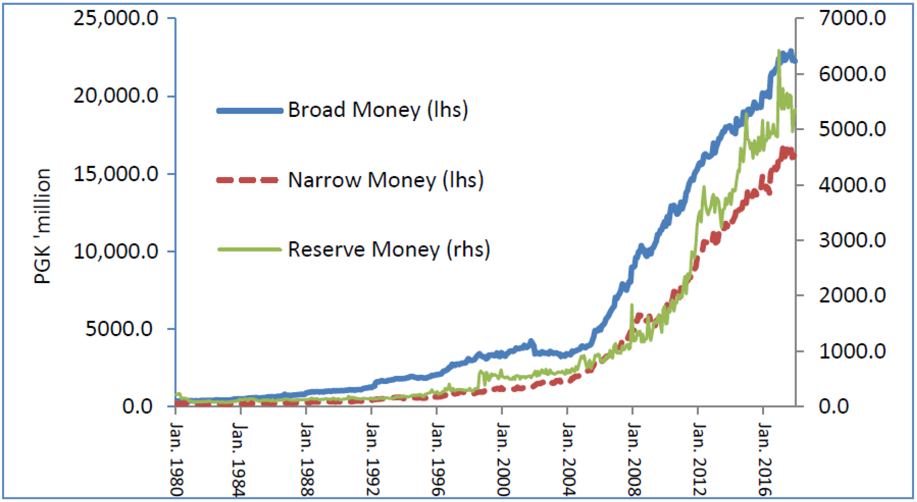
We first turn to the data to give us a preview of how the trend has been in PNG for the different money aggregates and the multipliers. The graphical presentation in Chart 1, shows strong co-movements between the money aggregates: for example, between the periods of 2004 and 2016 we see a surge as all grew strongly.
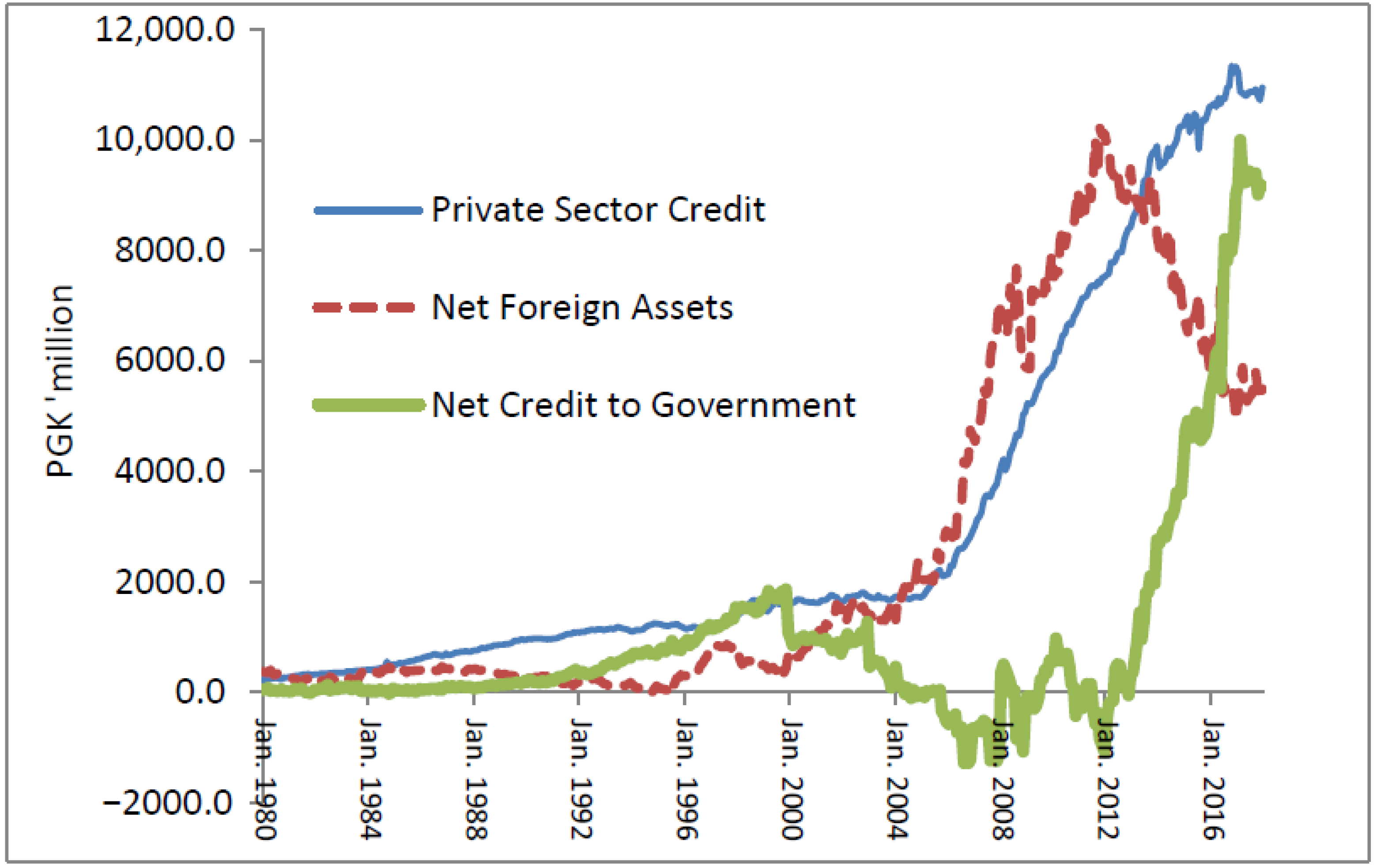
The determinants in Chart 2 show what this was attributed to: in periods of high commodity prices, the build-up in foreign assets contributed strongly to growth in monetary aggregates, while periods of low prices showed that either net credit to the Government or domestic borrowings by the Government was driving growth. Private sector credit growth remained persistent in between these surges. This suggests that deposits may be driven by external factors outside the Central Bank’s control, fueling credit growth.
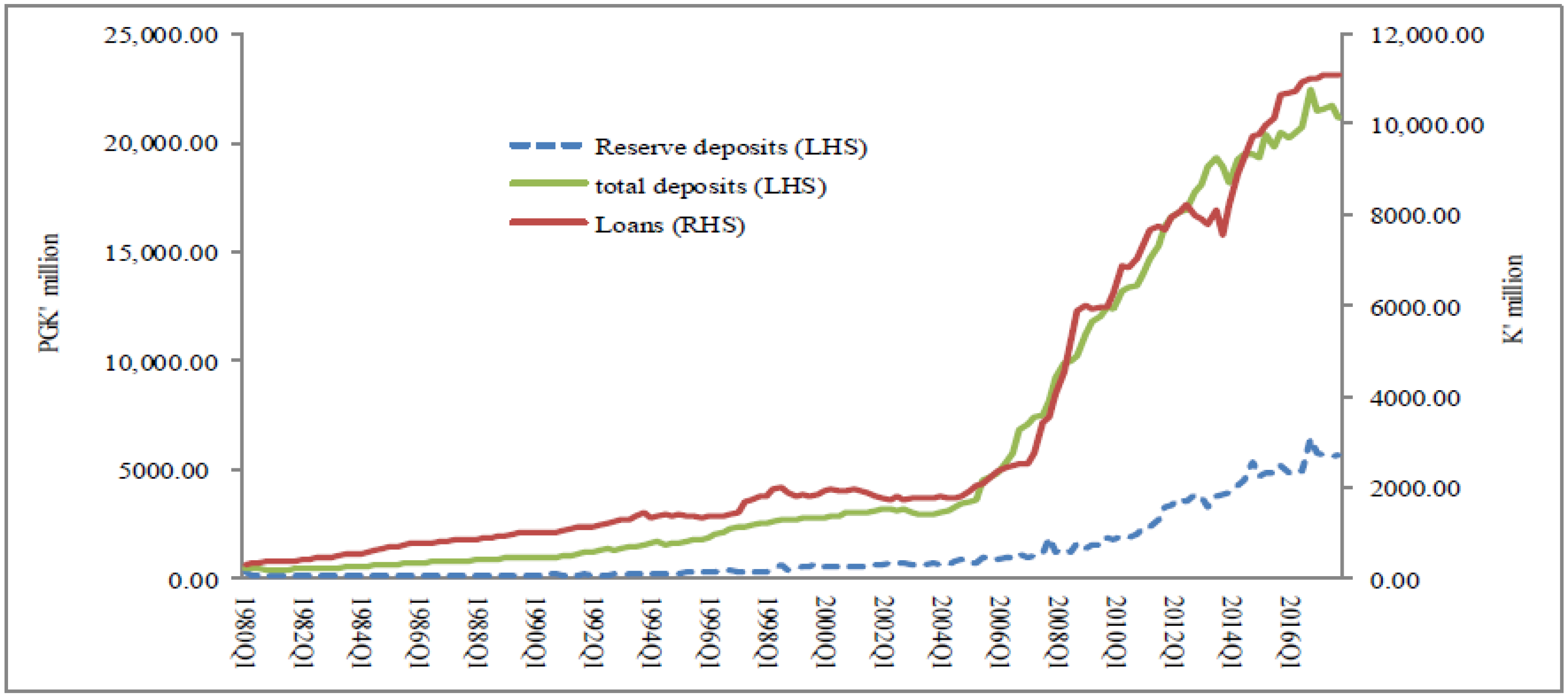
Looking specifically at bank data helps to filter the data from any changes in the methodology and compilation of money aggregates2 over the recent past and, importantly, examines the narrow bank lending channel. The graphical presentation in Chart 3 shows weak co-movements between reserve money and bank loans. On the other hand, loans are seen to move in tandem with changes in bank deposits, with the ratio almost constant over the period from 1980q1 to 2017q4. This simple visual inspection gives us an indication of what to expect from the relationship between the variables.
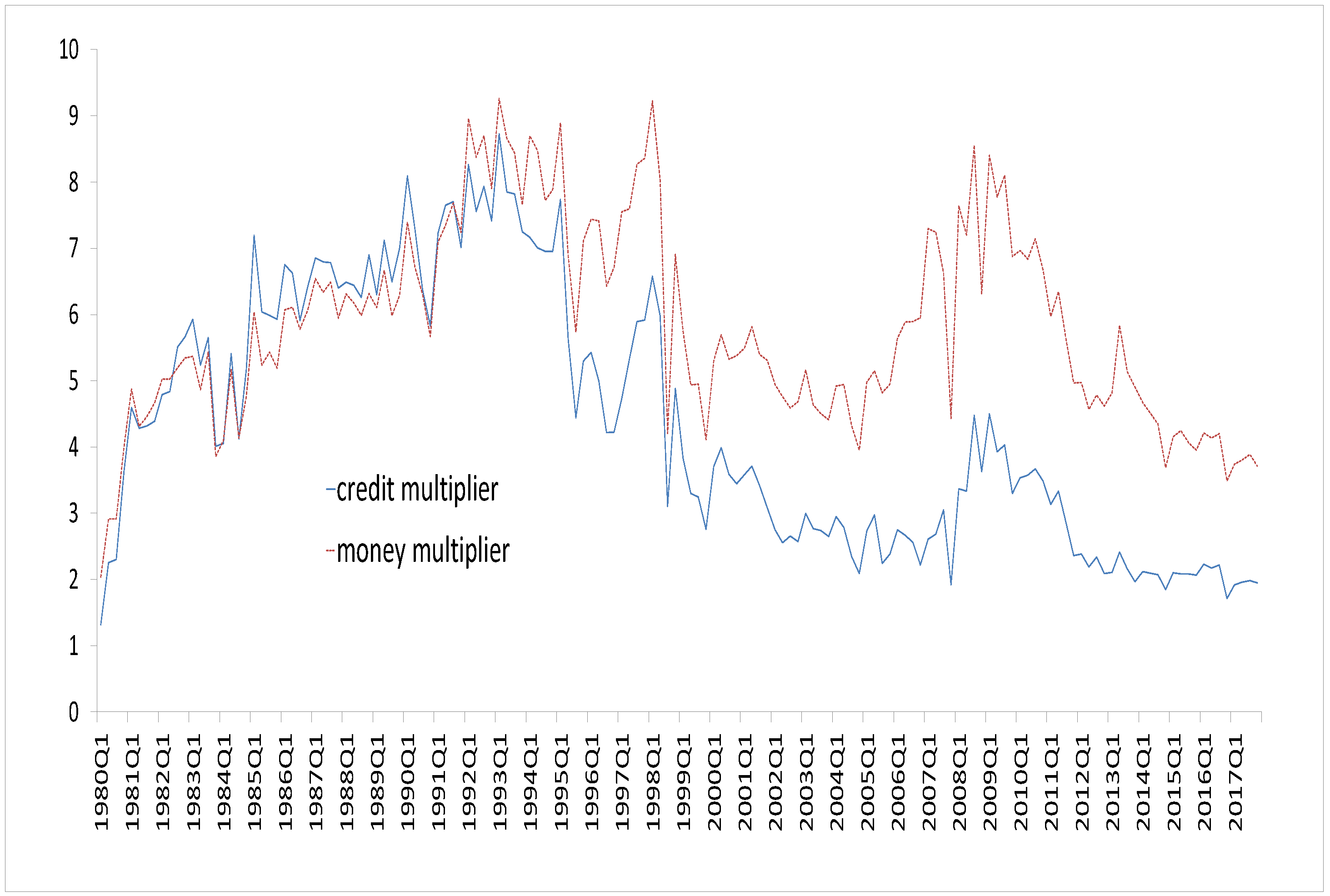
To put the recent trends into perspective, in 2016 total deposits were around PGK 20.0 billion while reserve deposits were just over PGK 5.03 billion, around 25% of total deposits. Bank loans were around PGK 11.0 billion. This suggests that reserve deposits alone are not sufficient to fund bank lending. There is a clear trend in the co-movements between loans and total deposits: both variables tend to track each other fairly closely over the sample period. If we take the ratios to measure the standard multipliers, a stable ratio between reserve money and the variables of loans and total deposits would indicate that the money multiplier holds. However, the ratios measured indicate that the relationships are unstable over the sample period (Chart 4). Prior to 1995, the credit multiplier was around the same size as the money multiplier. Thereafter, the credit multiplier fell below the money multiplier, suggesting the possibility of structural changes in the economy in which deposits and credit were driven by factors other than changes in the reserve money.
A notable feature in 1994 was the commencement of crude oil exports in PNG and the floating of the local currency (kina), which may have triggered an increase in the size of bank deposits in the banking system through the expansion of their holdings of foreign assets and liquidity. It is also important to note that we include in our measurement of money only the deposits of commercial banks. Hence, the omission of deposits of other deposit-taking institutions in this analysis makes our definition of money inadequate and as such, our conventional money multiplier concept is inappropriate. We follow the approach by Carpenter and Demiralp (2011) of narrowing the focus of our paper by examining the transmission from open market operations to money and bank lending. Hence, if the transmission is weak, we can make the inference that the transmission is ineffective and cannot influence domestic demand and inflation in the long run.
3. Data and Methodology
3.1. Data
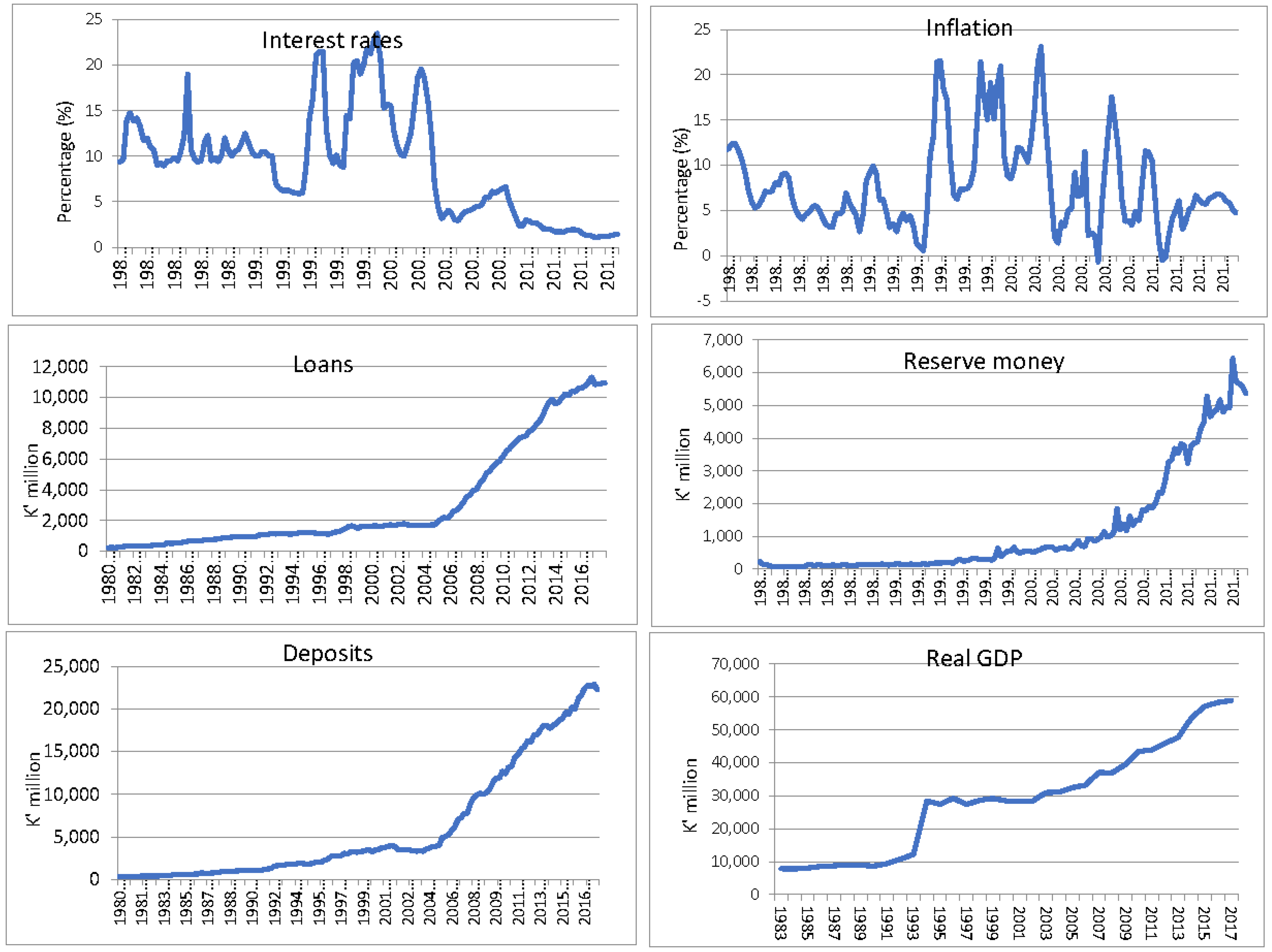
Following Carpenter and Demiralp (2011), we examine the inter-relationship between six variables: interest rate, inflation, loans, deposits, reserve money, and real GDP. All the variables are in quarterly series from 1980q1 to 2017q4 and are sourced from various publications of the Bank’s Quarterly Economic Bulletin. We use the 28-day Central Bank bill rate as the indicator for the Central Bank’s monetary policy variable. Normal convention would be to use the kina facility as this is the official policy rate. However, this been used sparingly, while the CBB rate has been predominantly used to influence domestic market interest rates. For prices, our model also uses CPI4 data. Currently, this is the only available official indicator of price pressures in PNG. For credit, the model uses loans extended by commercial banks, as they make up more than 85% of total loans extended by the financial sector and are the major target for monetary policy operations and conduct. For reserve money, our paper uses the reserve money deposits of commercial banks held at the Central Bank, as this is the explicit target variable in the Bank’s money market operations (Chart 5). For deposits, we use the total deposits of commercial banks. The model uses real GDP5 as there is no unemployment data available for PNG. Using the quadratic match averaging method of interpolation, we convert annual GDP data into quarterly frequency for the analysis. The variables are in nominal terms and expressed in log form and are not seasonally adjusted. Table 1 shows descriptive statistics of the variables used.
3.2. Methodology
For the most part, monetary economics focuses mainly on the behaviour of prices, money aggregates, nominal and real interest rates, and output (Garlach and Svensson Lars 2000). In this regard, the VAR models first developed by Sims (1980) have served as a primary tool in much of the empirical analysis of the interrelationships between these variables and for uncovering the impact of monetary phenomena on the real economy and business cycle (Stock and Watson 2001). This paper investigates the money multiplier in PNG using VARs, while applying a set of restrictions following Carpenter and Demiralp (2011) to uncover the relationships among the macroeconomic variables of interest.
We apply the ordinary least squares (OLS) method to estimate the system of vector autoregressions (VARs). Since we are interested only in the dynamic interrelationship between the variables and not the consistency in the coefficient estimates, the stationarity of the variables is not considered. It is assumed that, as demonstrated by Sims et al. (1990), the presence of unit roots should not affect the model selection process. When non-stationary variables are included in a VAR, the estimated regression results, including at levels, may become spurious. Variables are therefore stationarised or their levels tested for cointegration to determine whether a simple VAR can be estimated in the absence of cointegration, or whether a vector error correction model (VECM) is required, which combines both levels and first differences. Hence, variables are first tested for cointegration to select the best fit model. In our case the choice of a VAR including variables estimated in levels appears warranted in the light of the relatively small sample, which might make it quite difficult to separate difference-stationary variables from trend-stationary ones (e.g., Christiano and Eichenbaum 1990). Moreover, and for the same reasons, identification of the cointegration space would pose non-trivial problems. In addition, an important result in the literature (e.g., Sims et al. 1990) establishes the equivalence between a VAR representation in levels and a VECM representation. In essence, a VECM can always be thought of as a reparametrisation of a VAR specified in levels. Hence, in our analysis the variables enter the VAR system at levels and in natural log form. Consider the multivariate generalisation of an autoregressive process:
where ( vector containing each of the variables included in the VAR; ( vector of intercept terms; ( matrices of coefficients; and ( vector of error terms. The error terms are assumed to be serially uncorrelated with constant variance.
The variables entering the VAR system are treated as endogenous, which addresses the problem of endogeneity. The variables to be included in the VAR are usually selected according to the economic rationale or the relevant theory. For the functional form of the model, we turn to the Cholesky decomposition, propagating the shocks with the following ordering: real GDP; bank deposits; reserve money; loans; inflation; and interest rates.
The macroeconomic variables are ordered first and the CBB rate is ordered last because the policy rate is expected to respond to these variables contemporaneously at a quarterly frequency. The first variable in the system, GDP, represents unemployment; the assumption here is that deposits, reserve money, loans, prices, and the policy rate do not affect output contemporaneously—they are assumed to have lagged effects. The second variable, bank deposits, is assumed to affect output contemporaneously, while reserves, loans, prices, and the policy rate are assumed to have lagged effects. The third variable, reserve money, is assumed to affect bank deposits and output contemporaneously, while loans, prices, and the policy rate are assumed to have lagged effects. The fourth variable in the order, loans, is expected to affect reserves, deposits, and output contemporaneously, while prices and the policy rate are assumed to have lagged effects. Prices, the fifth variable in the order, is expected to affect all the variables in the system contemporaneously, except the policy rate. In essence, we are interested in the dynamic response of the economy to innovations in the policy rate, to measure the true structural response to monetary policy. In particular, we can see the monetary transmission mechanism unfold by examining the responses of bank balance sheet variables, including deposits and loans, and target variables, such as unemployment and inflation, to a policy shock. Our robustness checks reveal that the results are not sensitive to alternative orderings using the same sample period and variables (not shown). At this juncture, it is worth noting that the ordering does not capture the institutional dynamics of the Central Bank and how the monetary policy is expected to transmit under the reserve money framework practiced by the Bank. We attempt to account for this when we do the robustness test of the model using stylised facts. A few caveats are worth noting: the results may not be expected to follow the economic rational, given the limitations of some of the proxies used in our model. For instance, the interpolated GDP data are used in place of unemployment—there is an inverse relationship between both. While the US Fed Funds rate is an effective monetary policy tool relative to most developing economics, our proxy is not a policy rate per se. Additionally, the number of variables used and as a result the expected chain of causality, deviates given data availability. Finally, the VAR exercise is at a quarterly frequency, mainly because the price data are collected at this interval.
In the model specification the diagnostic tests, such as the lag length selection criteria, the stability of the VAR system for unit roots and the statistical properties of our residuals to ensure white noise were done to ensure reliability of the model estimates for a parsimonious model.
4. Empirical Results
We examined the results generated by the VAR6 system, which typically includes the impulse response function (IRF), the forecast error variance decompositions (FEVD), and the historical decompositions. Impulse responses showed how the different variables in the system responded to (identified) shocks; that is, the dynamic interactions between the endogenous variables in the VAR (p) process. Since we have ‘identified’ the structural VAR using the Cholesky ordering, the IRF will depict the responses to the structural shocks that have an economic interpretation. The FEVD provides information on the dynamics of the VAR system of equations and on how each variable responded and interacted to shocks in the other variables in the system. The seldom-used historical decomposition7 estimated the individual contributions of each structural shock to the movements in the variables used over the sample period.
4.1. Impulse Response Functions—Full Sample Analysis: 1980q1 to 2017q4
Since the focus of our analysis was centered on the dynamic relationship between the variables, the use of the impulse response function was appropriate. This use was to gauge both the unanticipated shocks to our monetary policy variables, of reserve money and interest rates, and the response generated by the variables in the system. Hence, the impulse response functions typically traced the effect of a shock to one endogenous variable on to the other variables in the VAR. In our initial analysis, we examined the data using the full sample period 1980q1 to 2017q4 while analysing the impact of reserve money, interest rates, and loans on one standard deviation shocks on the other variables in the VAR system. From the outset, although having a longer time series is advantageous for VARs, such a series is prone to structural changes over longer periods. For instance, in 1994 the exchange rate regime changed after 19 years from a fixed to a managed float. Additionally, since the early 1980s, several changes to the Bank’s intermediate policy targets coincided with monetary policy regime changes, such as shifting from money to credit growth, reserve money targeting after 2001, and mineral resource sector booms in more recent times. The Bank of PNG also liberalised its capital controls in 2005 by freeing up restrictions on large capital flows. Hence, the channels of monetary policy are also likely to have changed over this period and as such, our results may prove counterintuitive with respect to any economic rationale or theory that we may attempt to test.
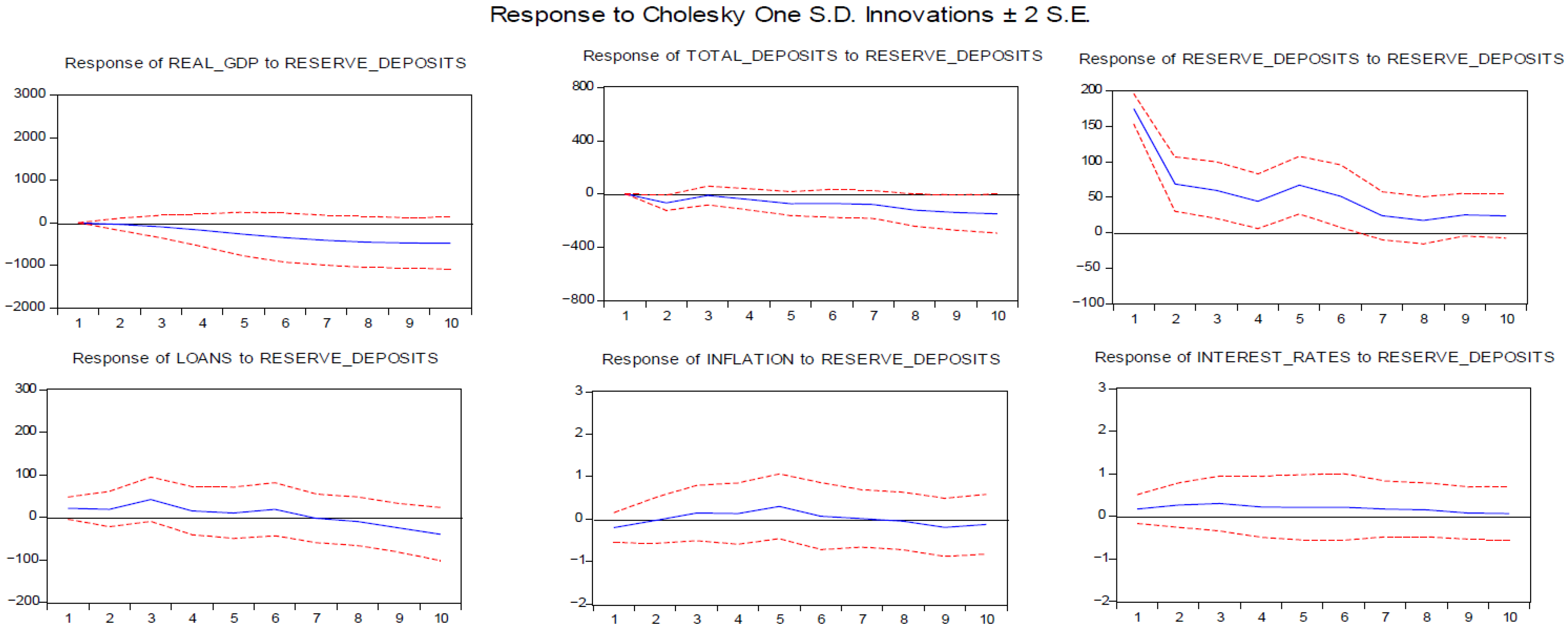
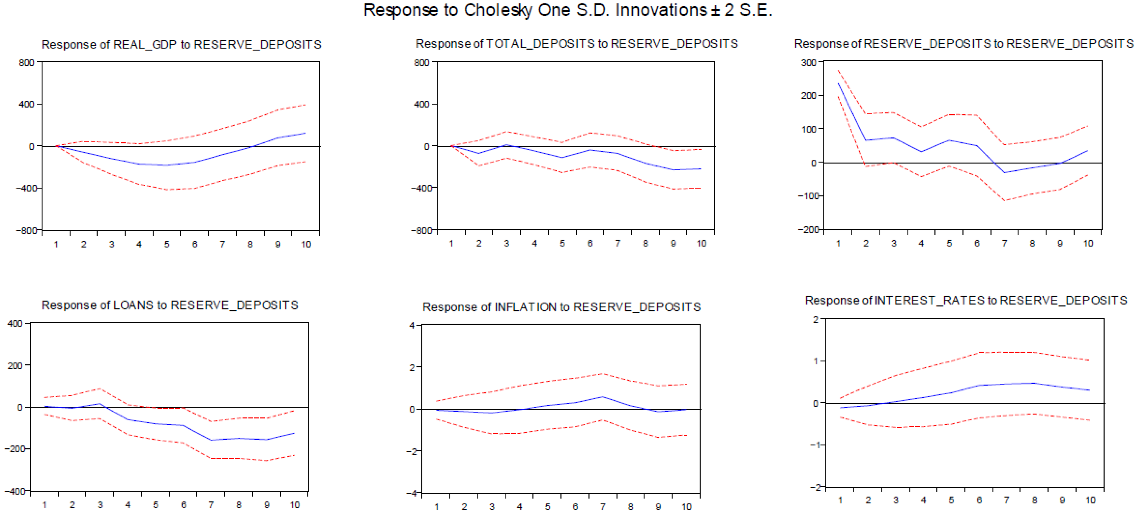
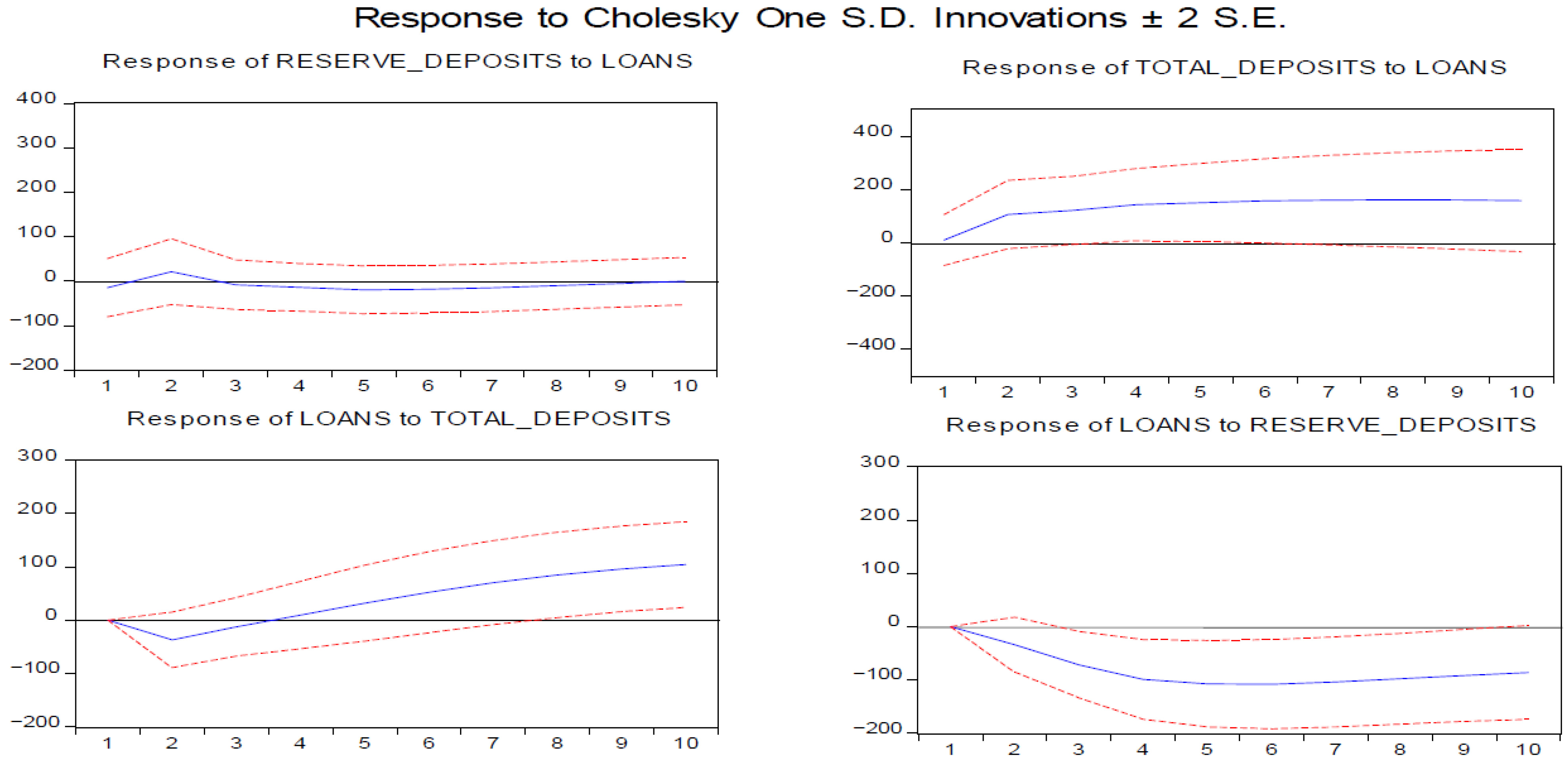
For the credit channel, the notion is that the “quantity of loanable funds” transmits monetary policy to the wider economy, otherwise known as the narrow bank lending channel (Meltzer 1995). However, results from our model in Figure 1 show that there was no real impact on loans despite an increase in reserve deposits; that is, an increase in quantity of loanable funds did not induce any increase in bank credit. On the contrary, the results are counterintuitive, showing a divergence, such that loans fell over the forecast horizon in response to a positive reserve money shock (bottom left panel). Should the transmission be effective, changes in the quantity of reserves through the Bank’s open market operations in the retirement or purchase of government securities should induce an increase in the amount of loanable funds that commercial banks can lend.
There are several plausible explanations for this, one of which is the exogenous demand-side factors not captured in this analysis, which include government spending and resource sector induced level of economic activity. Hence, while the amount of loanable funds increased, this may not necessarily lead to an increase in private sector borrowing. When we further examined the response of interest rates to the reserve money shock, there was no descendible response (bottom right panel). According to Monnet and Weber (2001), central banks do not control interest rates directly, but can adjust instruments that they control, such as reserves directly affecting the stock of money and subsequently the price of money, which is interest rates; however, this does not hold for our case. This suggests that the change in the volume of reserve deposits may not have been sufficiently large enough to induce a change in the price setting behaviour of commercial banks, with respect to changes in interest rates. This break in transmission is further evident in the lack of response of banking deposits to reserve money shocks (top middle panel). The notion here is that when firms draw down on the increase in the amount of loanable funds, the corresponding increase in loans should lead to a subsequent increase in bank deposits on the liabilities side. Our results suggest that there could be other exogenous factors, not necessarily reserve money, that may induce changes in the volume of bank deposits. This is particularly true for small open resource-rich economies like PNG.
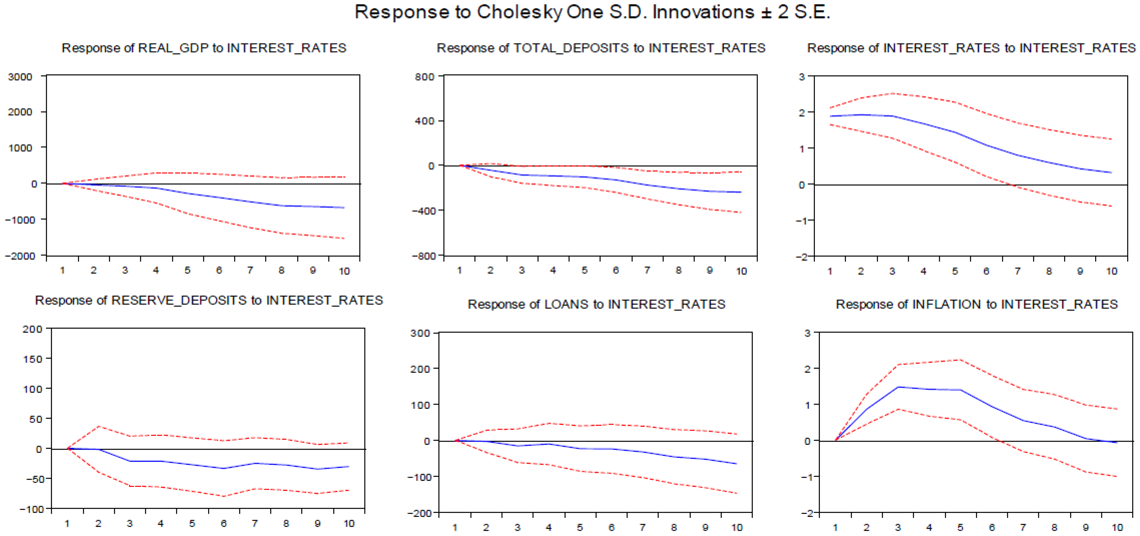
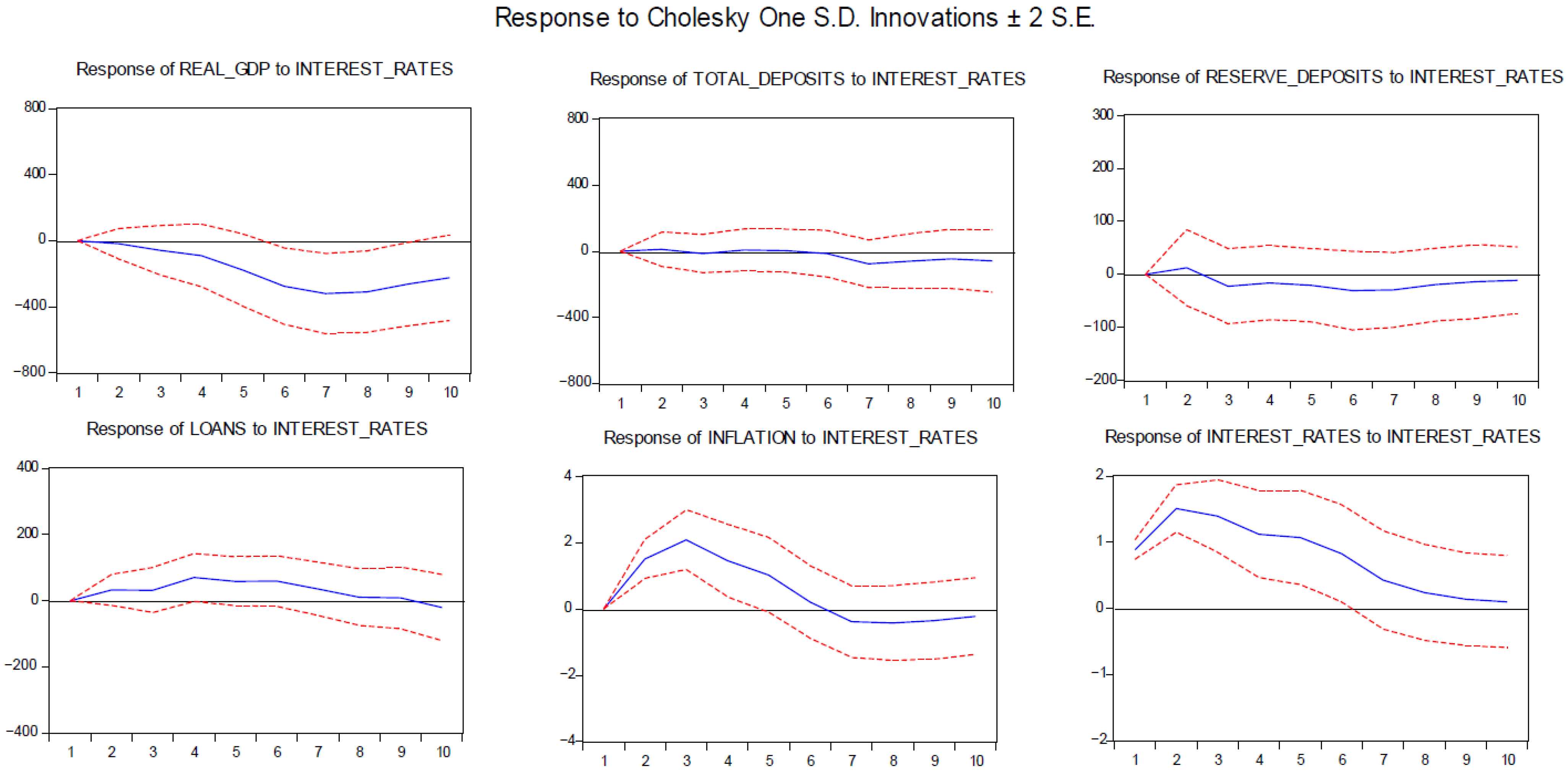
With respect to interest rate shocks, the interest rate adjusts to clear markets and influences borrowing and lending behaviour, according to the economic literature. By influencing the level of interest rates in the economy, monetary policy affects how much firms and households want to borrow (Mishkin 1996). The assumption here is that the interest rate is the exogenous policy variable. From the Cholesky ordering, interest rates affect the domestic variables contemporaneously. The results from the impulse response function (bottom middle panel, Figure 2) indicate that an increase in interest rates led to some contraction in bank loans as credit conditions tightened, while total deposits also contracted. This suggests that interest rates influence the borrowing behaviour of economic agents to some degree, as higher interest rates discourage borrowing. However, the impulse response function shows that there was no clear effect on reserve deposits from the interest rate shock (bottom left panel, Figure 2). A tighter liquidity condition through an increase in interest rates should lead to a fall in reserve deposits. These results suggest a breakdown in the behaviour of the two policy variables—that is, the price and volume of loanable funds that the Central Bank is assumed to have some influence over. The results may also suggest that there were inconsistencies and variations in the way monetary policy was conducted, as well as changes in the intermediate policy target variable over this period. Interestingly enough, we also observe a ‘price puzzle’8 in our results (bottom right panel) in the response in inflation to the interest rate shock (Eichenbaum and Evans 1995; Cushman and Zha 1997). There are two plausible explanations for this phenomenon; firstly, ‘price puzzles’ are usually observed in a closed economy setting, which is the case in our paper. In this regard, the open economy models have helped solve ‘puzzles’ in the behavioural relationship among macroeconomic variables that were often paradoxical relative to economic theory, often found in closed economy models, including ‘price puzzles’. These ‘puzzles’ are usually addressed by including additional variables that neutralise these unexplained or unusual outcomes. In most cases, including variables such as exchange rates, international oil, and commodity prices in the model to account for the ‘price puzzle’ help improve the empirical results (Grilli and Roubini 1995; Kim and Roubini 2000). Secondly, this may reflect the backward looking monetary policy reaction function of the Central Bank–the Bank response to inflation outcomes with a lag. Quarterly inflation data are usually received by the Bank with a lag of two to three months after the reporting quarter. Hence, there is a delayed response to price pressures, if any.
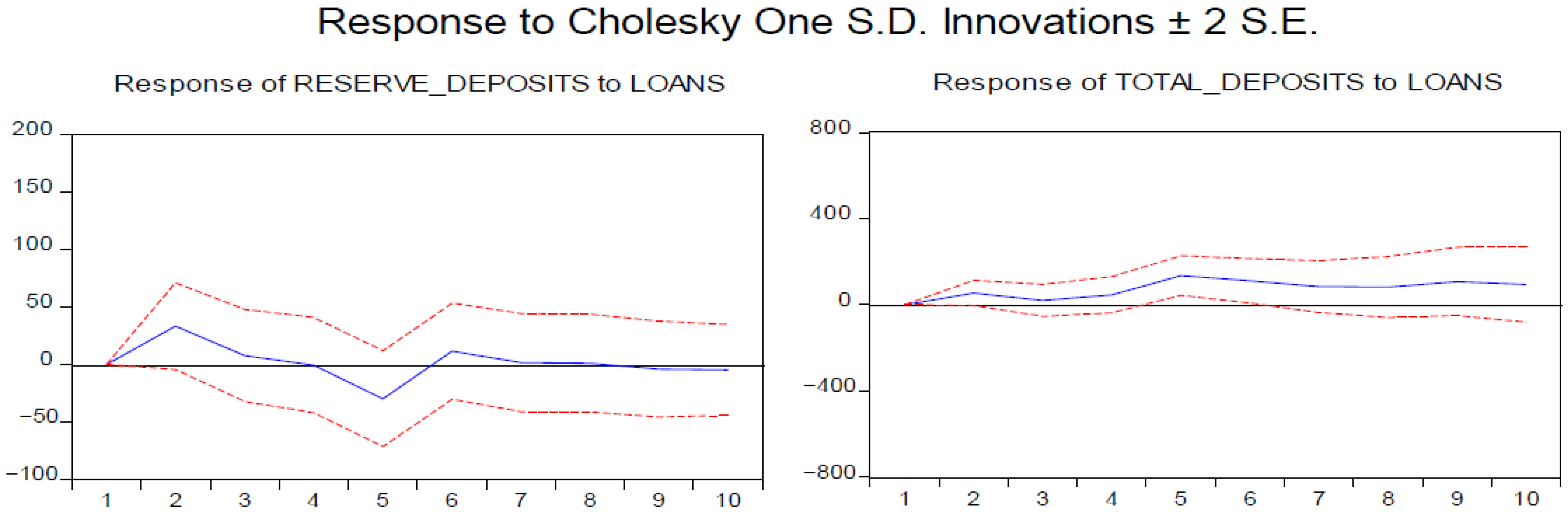
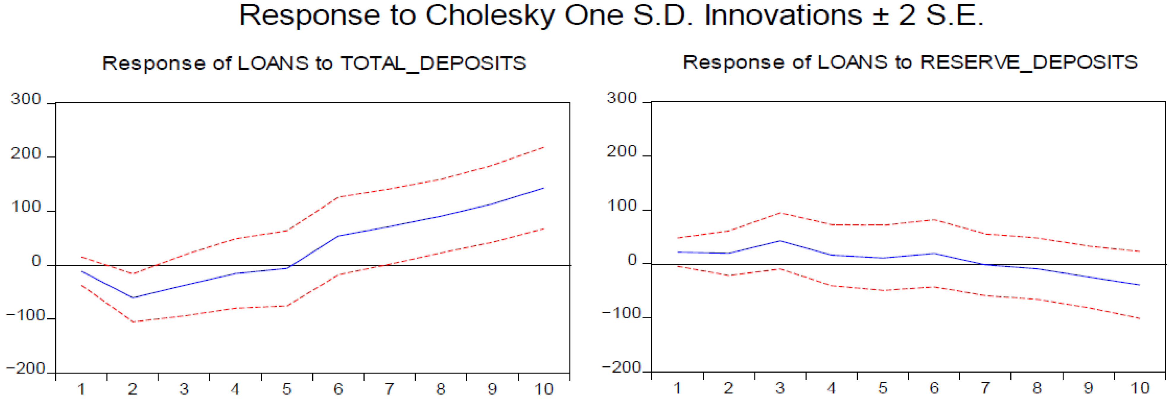
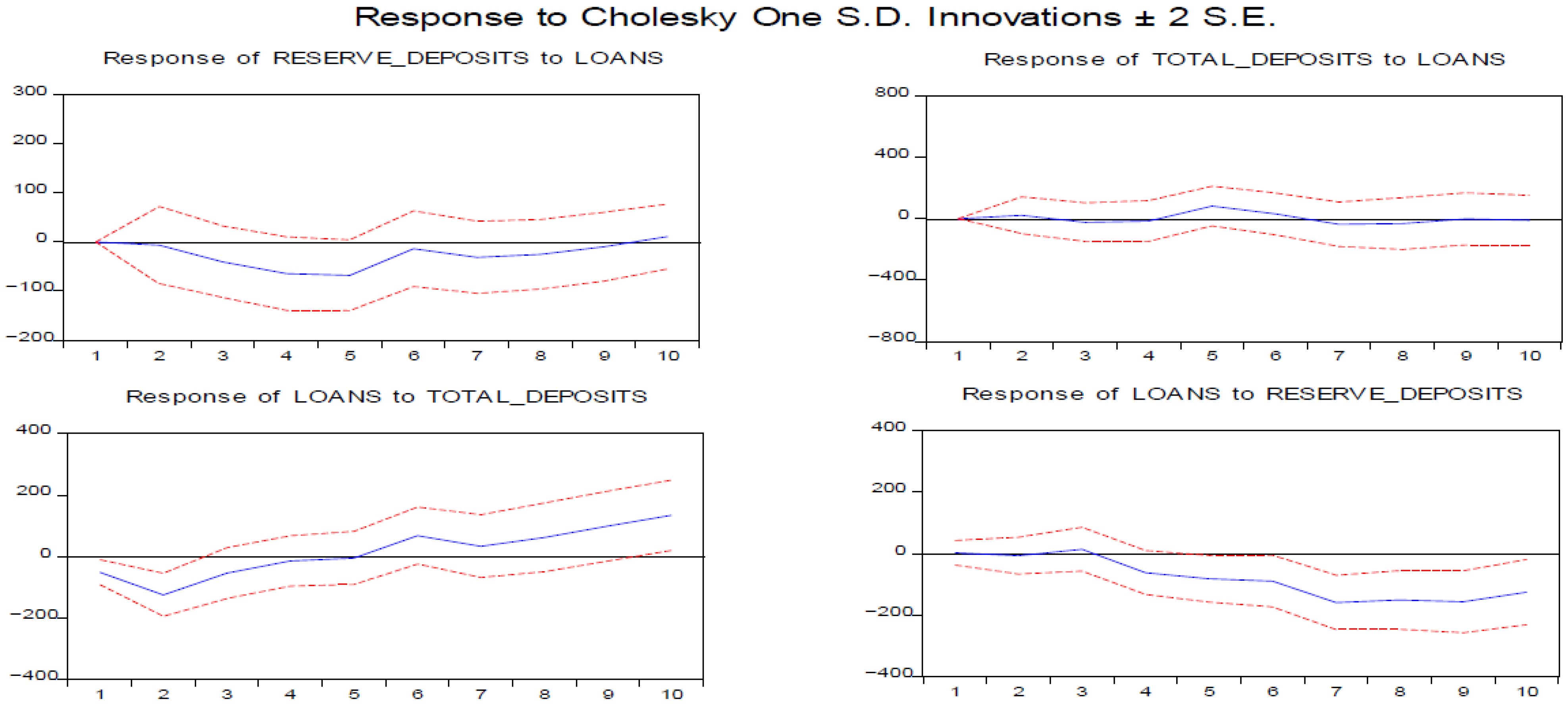
In Figure 3 and Figure 4 we investigate bank loans in closer detail by examining the impulse responses of loans to deposits and vice versa. In Figure 3, the right panel shows that total deposits increased in response to a bank loan shock, whereas reserve deposits barely responded to an increase in loans (left panel). Figure 4 (left panel) indicates that bank loans increased in response to an increase in total bank deposits; hence there is a clear link between deposits and loans. By contrast, counterintuitively bank loans decreased rather than increased in response to reserve money or loanable funds shocks (right panel). This is in contrast to the money multiplier effect and to our a priori expectations that bank loans should increase in response to an increase in reserve money or the amount of loanable funds. These suggest that bank loans are driven by exogenous demand-side factors and not supply-side (reserves).
4.2. Impulse Response Functions—Sub-Sample Analysis: 2000q1–2017q4
The Bank changed from using broad money aggregates as intermediate target variables to using reserve money or base money as the policy target variable after 2000, with the introduction of the Central Banking Act. This was consistent with the introduction of price stability as the objective of monetary policy in PNG. A policy interest rate target variable was also adopted as the signalling rate for the stance of policy. In essence, this sample period under analysis is warranted to cover only one policy regime, the reserve money framework. In this analysis we maintain the same variables, as well as their ordering, used in our full sample period.
In the examination of the sample periods from 2001q1 to 2017q4 under the reserve money regime, the impulse response function results (bottom left panel, Figure 5) indicate that loans fell in response to an increase in reserve money, while interest rates increased (bottom right panel). Total deposits also declined (top middle panel). Again, this is in contrast to a priori expectations regarding reserve money shock from the viewpoint of the ‘loanable funds’ theory: that is, the Central Bank creates money which then triggers credit and deposit creation. This is rejected by our results. So even under the Central Bank’s reserve money regime, there was still a lack of transmission from reserve money to total deposits and to loans extended.
In our examination of the interest rate channel, our model results in Figure 6 indicate a breakdown in the interest rate transmission: loans increased slightly in response to an interest rate shock (bottom left panel), but the increase in interest rates did not induce any response from total deposits. These results suggest that other macroeconomic factors are driving demand for credit while simultaneously contributing to an increase in interest rates. Although this goes beyond the scope of this paper, the key lies in the driver of inflation and how the interest rates respond to these shocks9. While open market operations were predominantly used during this period, the use of more direct instruments of monetary policy could have assisted, particularly during periods of high banking system liquidity.
The results from the impulse response functions in Figure 7 do not differ much compared to those of the full sample period, except that the total deposits’ response to increases in bank credit was weaker (top right panel). Several major events10 or external shocks that occurred during this period may have weakened the demand for loans while impacting bank deposits, which could explain this phenomenon. It is highly plausible that growth in deposits was driven by these factors, which attenuate the response of loans to monetary policy, lessening their sensitivity to reserve money and interest rate shocks.
4.3. Robustness Checking
We made an adaptation to the model by using lending rates, with reserve money as our explicit target policy variable,11 while changing the ordering of the variables to capture the stylised facts in the Bank’s reserve money framework. The supposed direction of the transmission is from reserve money, bank deposits, lending rates, bank loans, and inflation to real GDP. Through open market operations, the Central Bank either controls or targets some level of reserve money influencing the stock of deposits and subsequently the lending rates, bank loans, inflation, and aggregate demand (Monnet and Weber 2001).
For the sample period we re-examined the period 2000q1 to 2017q4. In this analysis, we investigated further using stylised facts with respect to the policy variables of interest, the shock propagation, and the chain of causality among the variables.
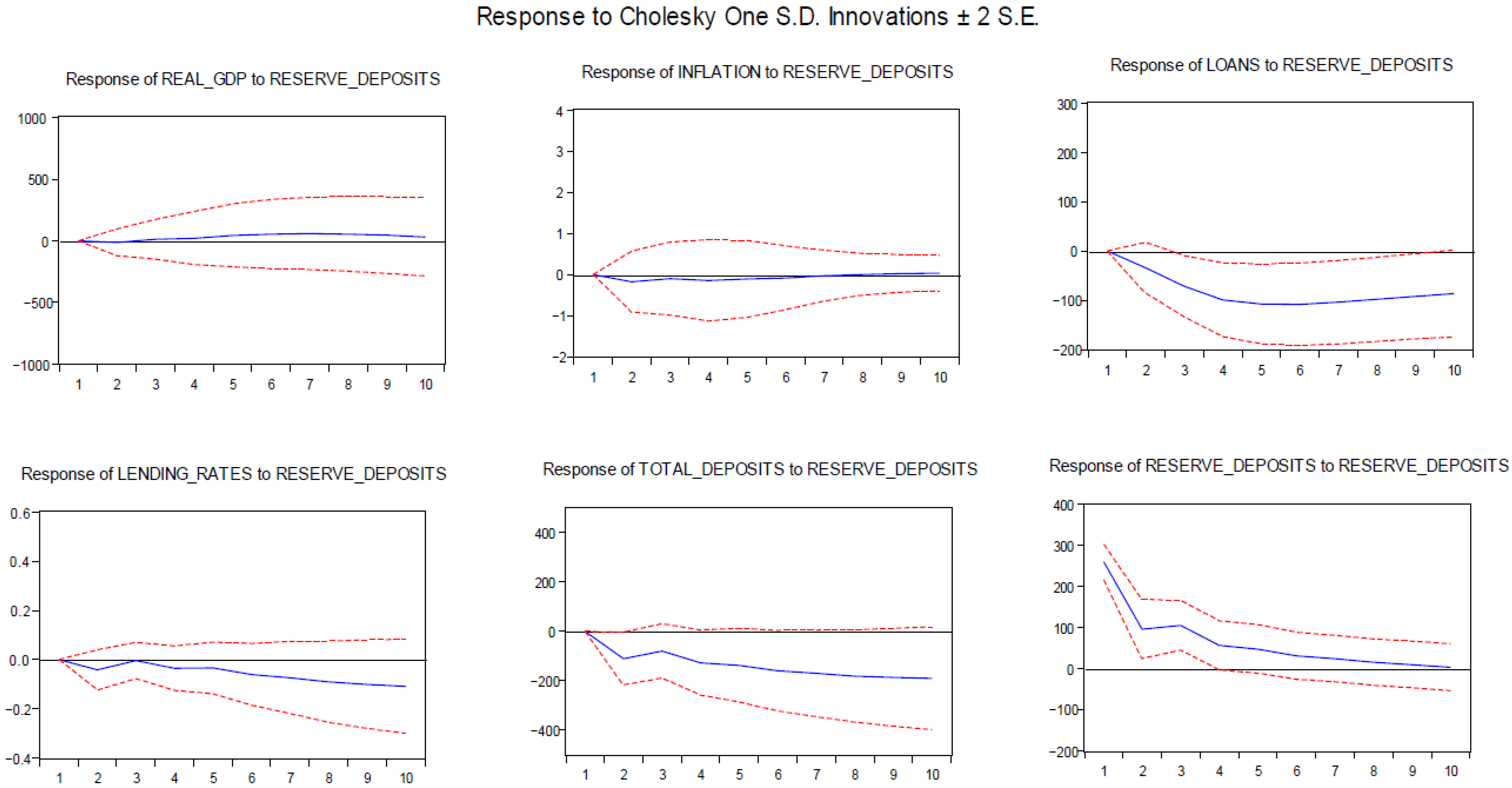
The results in Figure 8 show that a shock to reserve deposits is not consistent with our a priori expectations, such that total deposits declined (bottom middle panel), followed by a fall in commercial bank loans (top right panel), despite lower lending rates. These results further suggest that lending rates are not a major contributing factor with respect to bank borrowing behaviour. While the policy variable of reserve money increased given the positive shock, the impact extended only as far as inducing a fall in lending rates.
When we make a closer examination of the relationship between the variables, the results (Figure 9) show that the association between loans and deposits is in tandem, such that when there was a shock to loans the level of deposits increased and vice versa; that is, a shock to deposits prompted an increase in loans (bottom left and top right panels). On the other hand, a positive shock to reserve deposits prompted a fall in commercial bank loans despite a fall in lending rates (bottom right), while a shock to loans did not induce any response from reserve deposits (top left panel). The results in this policy scenario are statistically significant for most periods, which further suggest that the reserve money transmission to credit does not hold as indicated. In this case, it is plausible that the increase in bank deposits may have been driven by exogenous factors, causing an increase in banking system liquidity while fuelling demand for loans. Hence, this may have allowed firms and businesses to use their improved cash balances and profits during the boom periods to offset existing loans while refraining from borrowing from the commercial banks.
5. Conclusions and Policy Implications
This study investigated the monetary policy mechanisms and transmissions while examining the money multiplier concept and the credit channel in the case of PNG. The VAR model was estimated using quarterly data for the period 1980q1 to 2017q4. The estimation was conducted for the full and sub-sample periods. Our results show that the transmission is relatively weak: the volume of loans does not always respond to an increase in the supply of loanable funds. On the other hand, loans respond more to increases in bank deposits, suggesting that it might be the demand side of the economy that drives bank credit. Several plausible explanations go beyond the scope of this paper, one of which is the openness and vulnerability of the PNG banking sector to fiscal deficits and external price shocks. Another plausible explanation is that the foreign-owned banks may have access to liquidity and sources of financing from their parent holding companies abroad, which might make it challenging for the Central Bank to influence their lending behaviour. This also includes credit ceilings, imposed on certain industries by banks that may be considered as high risk. Overall, there is little evidence to suggest that the traditional monetary transmission mechanism, through bank credit, works through the Central Bank’s control of reserve money.
When examining the interest rates, we found that bank loans declined in response to an increase in interest rates; hence, interest rates play some part in influencing borrowing and lending behaviour. This holds for longer time series under the full sample period. However, when we examined a more recent and shorter sample period after the Central Bank’s reforms, 2000q1 to 2017q4, the results indicated a breakdown in this relationship, in that loans increased rather than decreased in response to increases in interest rates, while total bank deposits did not respond to increases in credit. The results using stylised facts for the same sample periods further suggest a weakness in the money multiplier, in that loans are more sensitive to changes in bank deposits than to reserve deposits, despite a fall in lending rates. From the discussion of the endogenous money creation viewpoint, credit and deposit growth do move in tandem, which may be a good way to look at the money creation process in PNG. While the literature has often pointed to financial innovations and increases in substitutes for money as the major factors in the breakdown in the multiplier, changes in external conditions appear to be an underlying factor as well for PNG.
Some policy implications emerge with respect to the Central Bank’s price stability mandate. If the focus is on interest rates, monetary operations may be centred on providing liquidity that yields an interest rate that is close to its policy rate. In this case, quantities, including reserve money, become endogenous to the price target. Alternatively, should the Central Bank seek further refinement to its reserve money framework, for a start, better and tighter control of liquidity conditions may be needed. This may require using a combination of both money market and direct policy instruments. The challenge is doing this consistently over sustained periods before any material outcomes are realised. Further research may include investigating the impact of international oil and commodity price shocks on the conduct of monetary policy, to better understand the exogenous shocks not captured in this study and to account for the ‘price puzzle’ depicted in our results of a closed economy model. Looking at a fiscal–monetary policy mix could also be useful in explaining how the budget cycle affects liquidity conditions that have been challenging for the Central Bank. In the meantime, this study provides systematically gained insights into the important question of whether the money multiplier holds in the case of PNG.
Author Contributions
Conceptualisation, M.O.; methodology, M.O.; software application using Eviews, M.O.; validation of results and text, M.O.; formal analysis, M.O.; investigation, M.O.; resources, M.O.; data curation, M.O.; writing—original draft preparation, M.O.; writing—review and editing, P.S.; visualisation, M.O. and P.S.; supervision, P.S.; project administration, P.S.; funding administration, P.S. All authors have read and agreed to the published version of the manuscript.
Funding
This research received no external funding.
Data Availability Statement
All data used are available and sourced from the statistical updates on Bank of Papua New Guinea official website at https://www.bankpng.gov.pg/statistics/quarterly-economic-bulletin-statistical-tables/ (accessed on 30 April 2018).
Acknowledgments
The authors acknowledge the Governor and technical staff of the Bank of Papua New Guinea and the team from Griffith University for the administrative, technical, and financial support in making possible the collaboration between both institutions, in one of many working papers to be published jointly. Especially, A Tarlok Singh’s mentoring and guidance is highly appreciated.
Conflicts of Interest
The authors declare no conflict of interest. The founding sponsors had no role in the design of the study; in the collection, analyses, or interpretation of data; in the writing of the manuscript, or in the decision to publish the results.
| 1 | See, for example, papers by Thenuwara and Morgan (2015); Tule and Ajilore (2016) and Disyatat (2011). |
| 2 | In 2008, the coverage on the compilation of monetary aggregates was extended to include non-banks. Prior to that, commercial bank deposits were the only source, albeit commercial banks make up more than 80% of total deposits at present. |
| 3 | Kina (K) is the local currency of PNG; the current rate is at around K1 per 0.30 US cents. |
| 4 | Sourced from the PNG National Statistical Office. |
| 5 | There is a structural break in 1994/1995 as depicted clearly in the graph. |
| 6 | The VAR models first developed by Sims (1980) are typically used to investigate the impact and relationship between monetary variables such as interest rate and money supply and prices and real output (Stock and Watson 2001). |
| 7 | Although historical decomposition was first developed by Sims (1980), the first study to use it was Beveridge and Nelson (1981). |
| 8 | Price increases rather than decrease in response to an increase in interest rates. |
| 9 | This can be viewed as external drivers that push prices up and subsequently credit demand. |
| 10 | 2008 GFC; 2005–2008 commodity price boom; 2009 PNG LNG construction phase |
| 11 | While the transmission framework includes interest rate as a policy variable, the practical aspects of the operations are arguably predominantly centred on influencing reserve money through the ESA of commercial banks. |
References
- Abdel-Baki, Monal. 2010. The Effects of Bank Reforms on the Monetary Transmission Mechanism in Emerging Market Economies: Evidence from Egypt. African Development Review 22: 526–39. [Google Scholar] [CrossRef]
- Arestis, Philip, and Malcolm Sawyer. 2002. The Bank of England Macroeconomic Model: Its Nature and Implications. Journal of Post Keynesian Economics 24: 529–45. [Google Scholar] [CrossRef]
- Armstrong, Angus, and Monique Ebell. 2015. Unconventional Monetary Policy: Introduction. National Institute Economic Review 234: R1–R4. [Google Scholar] [CrossRef] [Green Version]
- Badarudin, Zatul E., Ahmed M. Khalid, and Mohamed Ariff. 2009. Money Supply Behaviour in Emerging Economies: A Comparative Analysis. Journal of the Asia Pacific Economy 14: 331–50. [Google Scholar] [CrossRef]
- Baghestani, Hamid, and Tracy Mott. 1988. The money supply under alternative Federal Reserve operating procedures: An empirical examination. Southern Economic Journal 55: 485–93. [Google Scholar] [CrossRef]
- Beveridge, Stephen, and Charles R. Nelson. 1981. A new approach to decomposition of economic time series into permanent and transitory components with particular attention to measurement of the business cycle. Journal of Monetary Economics 82: 151–74. [Google Scholar] [CrossRef]
- Bhatti, Razzaque Hamza, and Muhammad Junaid Khawaja. 2018. The existence of a stable money multiplier in the small open economy of Kazakhstan. Journal of Economic Studies 45: 1211–23. [Google Scholar] [CrossRef]
- Carpenter, Seth, and Selva Demiralp. 2011. Money, reserves and the transmission of monetary policy: Does the money multiplier exist? Journal of Macroeconomics 34: 59–75. [Google Scholar] [CrossRef] [Green Version]
- Černohorská, Liběna. 2018. Endogeneity of money: The case of Czech Republic. Journal of International Studies 11: 155–68. [Google Scholar] [CrossRef]
- Christiano, Lawrence J., and Martin Eichenbaum. 1990. Unit Roots in Real GDP: Do We Know, and Do We Care? Carnegie-Rochester Conference Series on Public Policy 32: 37–61. [Google Scholar] [CrossRef] [Green Version]
- Crowe, Christopher, and Ellen E. Meade. 2007. The Evolution of Central Bank Governance around the World. The Journal of Economic Perspectives 21: 69–90. [Google Scholar] [CrossRef] [Green Version]
- Cushman, David O., and Tao Zha. 1997. Identifying monetary policy in a small open economy under flexible exchange Rates. Journal of Monetary Economics 39: 433–48. [Google Scholar] [CrossRef] [Green Version]
- Dan, Horațiu Sorin. 2013. The Exchange Rate Channel and Its Role within the Monetary Policy Transmission Mechanism. Studia Universitatis Babes-Bolyai. Studia Europaea 58: 133–48. [Google Scholar]
- David, Sali, and Alfred Nants. 2006. Monetary Policy Transmission Mechanisms in Papua New Guinea. Bank of Papua New Guinea Working Paper Series 2006/01. Port Moresby: Bank of Papua New Guinea, pp. 7–24. [Google Scholar]
- Disyatat, Piti. 2011. The Bank lending Channel revisited. Journal of Money, Credit and Banking 43: 713–30. [Google Scholar] [CrossRef]
- Dow, Sheila. 2016. The Political Economy of Monetary Reform. Cambridge Journal of Economics 40: 1363–76. [Google Scholar] [CrossRef]
- Eichenbaum, Martin, and Charles L. Evans. 1995. Some empirical evidence on the effects of shocks to monetary policy on exchange rates. Quarterly Journal of Economics 110: 975–1010. [Google Scholar] [CrossRef]
- Garlach, Stefan, and E. O. Svensson Lars. 2000. Money and Inflation in the Euro Area: A Case for Monetary Indicators? Working paper 8025. Cambridge: National Bureau of Economic Research, pp. 3–18. [Google Scholar]
- Grilli, V., and N. Roubini. 1995. Liquidity and Exchange Rates: Puzzling Evidence from the G-7 Countries. Working Papers 95-17. New York: New York University. [Google Scholar]
- Hafer, Rik W., Joseph H. Haslag, and Garett Jones. 2007. On money and output: Is money redundant? Journal of Monetary Economics 54: 945–54. [Google Scholar] [CrossRef] [Green Version]
- Ireland, Peter. 2004. Money’s role in the Monetary Business Cycle. Journal of Money, Credit and Banking 36: 969–83. [Google Scholar] [CrossRef] [Green Version]
- Jayaraman, Tiruvalangadu K., and Bert D. Ward. 2004. Is the money multiplier relevant in a small, open economy? Empirical evidence from Fiji. Pacific Economic Bulletin 19: 48–53. [Google Scholar]
- Jayaraman, Tiruvalangadu K., and Chee-Keong Choong. 2009. How does monetary policy transmission mechanism work in Fiji? International Review of Economics 56: 145–61. [Google Scholar] [CrossRef]
- Jayaraman, Tiruvalangadu K., and Chee-Keong Choong. 2010. How does monetary policy transmission mechanism work in Solomon Islands? Pacific Economic Bulletin 25: 76–95. [Google Scholar]
- Jha, Raghbendra, and Deba Prasad Rath. 2000. On the Endogeneity of Money Multiplier in India. Canberra: Australia South Asia Research Centre, pp. 4–30. [Google Scholar]
- Joyce, Michael, David Miles, Andrew Scott, and Dimitri Vayanos. 2012. Quantative Easing and Unconventional Monetary Policy—An Introduction. The Economic Journal 122: 271–88. [Google Scholar] [CrossRef] [Green Version]
- Kabundi, Alain, and Mpho Rapapali. 2019. The Transmission of Monetary Policy in South Africa Before and After the Global Financial Crisis. The South African Journal of Economics 87: 464–89. [Google Scholar] [CrossRef]
- Keynes, John Maynard. 1930. A Treaties on Money. New York: St Martin’s Press. [Google Scholar]
- Kim, Soyoung, and Roubini Nouriel. 2000. Exchange rate anomalies in the industrial countries: A solution with a structural VAR approach. Journal of Monetary Economics 45: 561–86. [Google Scholar] [CrossRef]
- Leeper, Eric M., and Jennifer E. Roush. 2003. Putting ‘M’ Back in Monetary Policy. Journal of Money, Credit and Banking 35: 1257–64. [Google Scholar] [CrossRef]
- Lombardi, Domenico, Pierre Siklos, and Samantha St. Amand. 2018. A Survey of the International Evidence and Lessons Learnt about Unconventional Monetary Policies: Is a new normal in our Future? Journal of Economic Surveys 32: 1229–56. [Google Scholar] [CrossRef]
- Max, Hanish. 2017. The Effectiveness of Conventional and Unconventional Monetary Policy: Evidence from a Structural Dynamic Factor Model for Japan. Journal of International Money and Finance 70: 110–34. [Google Scholar]
- Meinusch, Annette, and Peter Tillmann. 2016. The macroeconomic impact of unconventional monetary policy shocks. Journal of Macroeconomics 47: 58–67. [Google Scholar] [CrossRef] [Green Version]
- Meltzer, Alan. H. 1995. Money, credit and (other) transmission process: A Monetarist Perspective. The Journal of Economic Perspective 9: 49–72. [Google Scholar] [CrossRef]
- Meltzer, Alan H. 2001. The Monetary Transmission Process: Recent Developments and Lessons for Europe. Edited by Deutsche Bundesbank. London: Palgrave, pp. 112–30. [Google Scholar]
- Mishkin, Frederic S. 1995. Symposium on the Monetary Transmission Mechanism. The Journal of Economic Perspectives 9: 3–10. [Google Scholar] [CrossRef] [Green Version]
- Mishkin, Frederic S. 1996. The Channels of Monetary Transmission: Lessons for Monetary Policy. Working Paper Series 5464. Cambridge: National Bureau of Economic Research (NBER), pp. 4–24. [Google Scholar]
- Monnet, Cyril, and Warren E. Weber. 2001. Money and interest rates. Federal Reserve Bank of Minneapolis Quarterly Review 25: 2–13. [Google Scholar]
- Moore, B. J. 1989. Horizontalists and Verticalists: The Macroeconomics of Credit Money. Cambridge: Cambridge University Press. [Google Scholar]
- Narayan, Paresh Kumar, Seema Narayan, Sagarika Mishra, and Russell Smyth. 2012. An analysis of Fiji’s monetary policy transmission. Studies in Economics and Finance 29: 52–70. [Google Scholar] [CrossRef]
- Nelson, Edward. 2002. Direct effects of base money on aggregate demand: Theory and evidence. Journal of Monetary Economics 49: 687–708. [Google Scholar] [CrossRef]
- Oguzhan, Cepni, and Guney Ibraham Ethem. 2017. Endogeneity of Money Supply: Evidence from Turkey. International Journal of Finance & Banking Studies 6: 1–10. [Google Scholar]
- Peiris, Shanaka J., and Ding Ding. 2012. Global Commodity Prices, Monetary Transmission, and Exchange Rate Pass-through in the Pacific Islands. Washington, DC: IMF Working Paper Series WP/12/176, pp. 3–13. [Google Scholar]
- Prasad, Eswar S., Gill Hammond, and Ravi Kanbur. 2009. Monetary Policy Challenges for Emerging Market Economies. In Brookings Global Economy and Development Working Paper No. 36. Ithaca: Cornell University. [Google Scholar] [CrossRef]
- Rachma, M. S. 2011. Endogeneity of money supply in Indonesia. Economic Journal of Emerging Markets 2: 277–88. [Google Scholar]
- Robbins, Lionel. 1932. An Essay on the Nature and Significance of Economic Science. London: Macmillan. [Google Scholar]
- Salachas, Evangelos N., Nikiforos T. Laopodis, and Georgios P. Kouretas. 2017. The bank-lending channel and monetary policy during pre-and post-2007 crisis. Journal of International Financial Markets 47: 176–87. [Google Scholar] [CrossRef]
- Sengupta, Nandini. 2014. Changes in Transmission Channels of Monetary Policy in India. Economic and Political Weekly 49: 62–71. [Google Scholar]
- Sims, Christopher A. 1980. Macroeconomics and reality. Econometrica 48: 1–48. [Google Scholar] [CrossRef] [Green Version]
- Sims, Christopher A., James H. Stock, and Mark W. Watson. 1990. Inference in linear time series models with some unit roots. Econometrica 58: 113–44. [Google Scholar] [CrossRef]
- Stauffer, Robert. 2006. An innovative Money Multiplier. The American Economist 50: 58–64. [Google Scholar] [CrossRef]
- Stock, James H., and Mark W. Watson. 2001. Vector Autoregressions. Journal of Monetary Economics 44: 293–335. [Google Scholar] [CrossRef]
- Thenuwara, Wasanthi, and Bryan Morgan. 2015. Monetary targeting in Sri Lanka: How much control does the central bank have over the money supply? Journal of Economics and Finance 41: 276–96. [Google Scholar] [CrossRef]
- Tule, K. Moses, and Taiwo O. Ajilore. 2016. On the stability of the money multiplier in Nigeria: Co-integration analyses with regime shifts in banking system liquidity. Cogent Economics & Finance 4: 2–16. [Google Scholar]
- Yang, Yongzheng, Matt Davies, Shengzu Wang, Jonathan Dunn, and Yiqun Wu. 2012. Monetary policy transmission and macroeconomic policy coordination in Pacific island countries. Asia Pacific Economic Literature 13: 46–68. [Google Scholar] [CrossRef]
Chart 1.
Money aggregates. Source: Bank of Papua New Guinea.

Chart 2.
Determinants of money supply. Source: Bank of Papua New Guinea.

Chart 3.
Bank deposits and loans. Source: Bank of Papua New Guinea.

Chart 4.
Credit and money multipliers. Source: Bank of Papua New Guinea.

Chart 5.
Major monetary and macroeconomic aggregates. Source: Bank of Papua New Guinea.

Figure 1.
Impulse response to reserve money shocks: credit channel. Source: Authors’ calculations.

Figure 2.
Impulse response to interest rate shocks: interest rate channel. Source: Authors’ calculations.
Figure 2.
Impulse response to interest rate shocks: interest rate channel. Source: Authors’ calculations.

Figure 3.
Impulse responses of liabilities to loans. Source: Authors’ calculations.

Figure 4.
Impulse responses of loans to liabilities. Source: Authors’ calculations.

Figure 5.
Impulse response to reserve money shocks: credit channel. Source: Authors’ calculations.

Figure 6.
Impulse response to interest rate shocks: interest rate channel. Source: Authors’ calculations.
Figure 6.
Impulse response to interest rate shocks: interest rate channel. Source: Authors’ calculations.

Figure 7.
Impulse response functions: loans to liabilities. Source: Authors’ calculations.

Figure 8.
Impulse response function: robustness checking. Source: Authors’ calculations.

Figure 9.
Impulse response function: response of loans to liabilities. Source: Authors’ calculations.
Figure 9.
Impulse response function: response of loans to liabilities. Source: Authors’ calculations.


Table 1.
Descriptive statistics.
| Real GDP | Deposits | Reserve Money | Loans | Interest Rate | Inflation | |
|---|---|---|---|---|---|---|
| Mean | 288,770.08 | 6352.134 | 1273.791 | 3383.245 | 8.769071 | 7.650931 |
| Median | 29,099.08 | 2832.050 | 553.8000 | 1789.800 | 9.220000 | 6.244999 |
| Maximum | 58,958.82 | 22,434.70 | 6431.382 | 11,099.90 | 23.50000 | 23.12333 |
| Minimum | 7788.395 | 425.2000 | 79.20000 | 469.6000 | 1.110000 | −0.675357 |
| Std. Dev | 15,998.00 | 7038.816 | 1656.535 | 3295.049 | 5.895791 | 5.129250 |
| Skewness | 0.198255 | 1.084331 | 1.553272 | 1.184906 | 0.641266 | 1.151765 |
| Kurtosis | 2.065634 | 2.583802 | 4.109951 | 2.890473 | 2.643822 | 3.861053 |
| Jarque–Bera | 6.009570 | 28.44515 | 63.48188 | 32.83003 | 10.33521 | 35.27802 |
| Probability | 0.049549 | 0.000001 | 0.00000 | 0.0000 | 0.005698 | 0.00000 |
| Sum | 4,027,811 | 889,298.7 | 178,330.8 | 473,654.3 | 1227.670 | 1071.130 |
| Sum Sq. Dev | 356 × 1010 | 6.89 × 10⁹ | 3.81× 10⁸ | 151 × 109 | 4831.689 | 3656.979 |
| Observations | 140 | 140 | 140 | 140 | 140 | 140 |
Source: Authors’ calculations.
Publisher’s Note: MDPI stays neutral with regard to jurisdictional claims in published maps and institutional affiliations. |
© 2021 by the authors. Licensee MDPI, Basel, Switzerland. This article is an open access article distributed under the terms and conditions of the Creative Commons Attribution (CC BY) license (https://creativecommons.org/licenses/by/4.0/).
Share and Cite
MDPI and ACS Style
Ofoi, M.; Sharma, P. Does the Money Multiplier Hold in Pacific Island Countries? The Case of Papua New Guinea. J. Risk Financial Manag. 2021, 14, 449. https://0-doi-org.brum.beds.ac.uk/10.3390/jrfm14090449
AMA Style
Ofoi M, Sharma P. Does the Money Multiplier Hold in Pacific Island Countries? The Case of Papua New Guinea. Journal of Risk and Financial Management. 2021; 14(9):449. https://0-doi-org.brum.beds.ac.uk/10.3390/jrfm14090449
Chicago/Turabian StyleOfoi, Mark, and Parmendra Sharma. 2021. "Does the Money Multiplier Hold in Pacific Island Countries? The Case of Papua New Guinea" Journal of Risk and Financial Management 14, no. 9: 449. https://0-doi-org.brum.beds.ac.uk/10.3390/jrfm14090449