
Good Practice Principles in Modelling Defined Contribution Pension Plans


1
Business School, Durham University, Mill Hill Lane, Durham DHL 3LB, UK
2
Pensions Institute, Bayes Business School, City University of London, 106 Bunhill Row, London EC1Y 8TZ, UK
*
Author to whom correspondence should be addressed.
J. Risk Financial Manag. 2022, 15(3), 108; https://0-doi-org.brum.beds.ac.uk/10.3390/jrfm15030108
Submission received: 24 January 2022
/
Revised: 17 February 2022
/
Accepted: 18 February 2022
/
Published: 26 February 2022
(This article belongs to the Special Issue Macroeconomic Modelling)
Abstract
:We establish 16 good practice principles for modelling defined contribution pension plans. These principles cover the following issues: model specification and calibration; modelling quantifiable uncertainty; modelling member choices; modelling member characteristics, such as occupation and gender; modelling plan charges; modelling longevity risk; modelling the post-retirement period; integrating the pre- and post-retirement periods; modelling additional sources of income, such as the state pension and equity release; modelling extraneous factors, such as unemployment risk, activity rates, taxes and welfare entitlements; scenario analysis and stress testing; periodic updating of the model and changing assumptions; and overall fitness for purpose.
Keywords:
defined contribution pension plans; PensionMetrics methodology; OECD Roadmap for the Good Design of Defined Contribution Pension Plans; EIOPA Good Practices on Information Provision for DC Schemes: Enabling Occupational DC Scheme Members to Plan for RetirementJEL Classification:
C15; C18; C63; C68; D14; D911. Introduction
If a defined contribution (DC) pension plan is well designed, it will be a single, integrated financial product that delivers, at reasonable cost to the plan member, a pension that provides a high degree of retirement income security. This pension should provide an adequate replacement income for the remaining life of the plan member (and possibly also a spouse or partner) and should remove the risk that the member outlives his or her resources. A well-designed plan will therefore be designed from back to front, that is, from desired outputs to required inputs (see Blake 2008).
We have spent over two decades thinking about the design of DC plans as well as the modelling of different aspects of the design and, over the course of this work, we have conceived and built a DC pension simulation model called PensionMetrics (see Blake et al. 2001, 2003). The model is stochastic, which means that it involves underlying processes that are generated randomly and enables us to quantify uncertainty, reflecting the fact that the future is uncertain. We can also regard this model as providing what is sometimes referred to as a stochastic scenario analysis.
What we outline here is a set of good practice modelling principles, based on our experience in DC modelling, and key points are illustrated with results from the PensionMetrics model.
To organise the discussion, we start with a simple and familiar DC pension problem; we then gradually incorporate more features to make the model more realistic. So, for example, we take into account specific information about a plan member such as age, gender, occupation, marital status, existing wealth and debts, and attitude to risk. In other words, we can model a plan that is tailor-made to each plan member. By also taking into account the member’s non-pension assets and liabilities, we can model not only a pension plan, but also a wealth management plan, which is a plan that manages the individual’s wealth over his or her life cycle. It is important to recognise that a formal pension plan is only one of the ways—albeit a key one—of providing resources in retirement. Here, however, we will concentrate on the pension plan. We will also focus exclusively on DC plans, which the majority of individuals now have if they work for a private-sector employer.1
It is important to recognise that we are not offering pension-planning advice nor are we discussing what the principles of good pension-planning advice should be. Advice on what plan members should do is a separate matter altogether, as is the advice that might come from using a pension simulation model. Rather, we are concerned with modelling, i.e., we make a set of assumptions about economic scenarios, member decisions and so forth, and, based on those assumptions, the model projects the prospective outputs. Those projections can then be used to guide both the plan design and member choices, but our focus is on modelling or, more particularly, the principles of good modelling. We will establish these as our discussion progresses.
We begin with some general comments about model specification and calibration.
2. Model Specification and Calibration
Any DC pension model should be built using plausible assumptions about the stochastic processes driving key variables (such as asset prices, interest rates and mortality rates) and these processes should have empirically plausible calibrations. These calibrations would cover, inter alia, the risk premia on growth assets such as equities, the interest-rate process and the mortality process, across the whole time horizon relevant for the plan member.
This time horizon will extend not just to the planned date of retirement, but until the member’s maximum anticipated age of death; the horizon is therefore very long. Thus, a plan member aged 25 will have a potential horizon of over 75 years.
Key assumptions about processes and calibrations should be transparent. Such transparency helps ensure that the modelling process meets evolving good-practice standards in due diligence.
- Principle 1: The underlying assumptions in the model should be plausible, transparent and internally consistent.
Plan sponsors should be able to demonstrate that the processes and calibrations used have been considered by appropriate experts; they should also have protocols in place to verify or backtest model projections.2
- Principle 2: The model’s calibrations should be appropriately audited or challenged, and the model’s projections should be subject to backtesting.
3. Modelling Quantifiable Uncertainty
DC models should aim to produce reliable projections of likely outcomes (such as the pension amount or replacement ratio at retirement3) and should also take account of the probabilities associated with projected outcomes. In short, DC models should deal with quantifiable uncertainty.4
- Principle 3: The model must be stochastic and be capable of dealing with quantifiable uncertainty.
This principle implies that purely deterministic projections are highly problematic—and, indeed, wrong in principle.
For example, the UK regulator, the Financial Conduct Authority (FCA), requires plan sponsors to provide deterministic projections of pension fund values for hypothetical pension fund returns of 2%, 5% and 8% (Financial Conduct Authority 2021). However, such projections are highly misleading as they provide no indication of the likelihoods or probabilities of achieving such returns.5 Indeed, one can easily be faced with situations in which the probability of achieving an annual return of 8% over an extended investment horizon is essentially zero.
The FCA’s requirement that plan sponsors produce such projections can therefore be misleading, because it can suggest, to plan members, that such outcomes are plausible when they might not be.
The need to address quantifiable uncertainty suggests that the natural numerical method to use would be some form of stochastic simulation or Monte Carlo analysis. It also raises the need for suitable risk metrics. For example, a DC model might produce estimates of the 5th percentile point of the distribution of the simulated output variable of interest (this is known as the 5% value-at-risk or VaR) or estimates of the 90% prediction interval for the output variable of interest. As we show below, these risk metrics can be illustrated graphically using a variety of charts, including probability density charts and fan charts.6
- Principle 4: A suitable risk metric should be specified for each output variable of interest, especially one dealing with downside risk. Examples would be the 5% value-at-risk and the 90% prediction interval. These risk metrics should be illustrated graphically using appropriate charts.
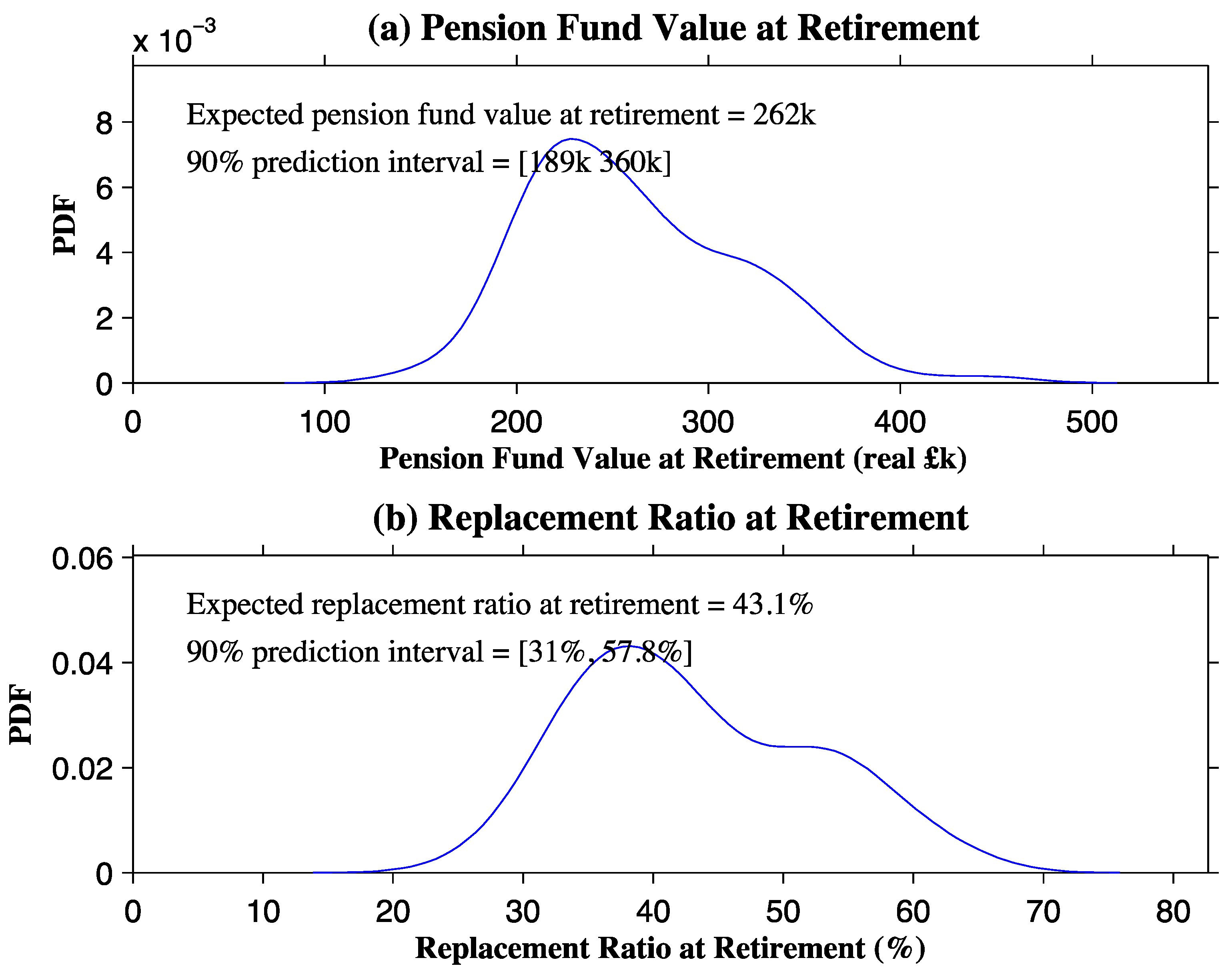
Two examples are given in Figure 1 which show the simulated pension fund at retirement (panel (a)) and the simulated replacement ratio at retirement (panel (b)) based on an assumed ‘base case’ and set of underlying assumptions about relevant driving processes and other relevant parameters (of which more below).
For our base case, we assume a single male, who starts contributing to a DC pension plan at age 25. We assume a total contribution rate of 9% of salary, comprising a 5% employee contribution and a 4% employer contribution. We also assume that he has a starting salary of £24,000, faces an ‘average’ career salary profile for the UK (see Figure 2) and anticipates working straight through to retirement at age 65. We further assume that his asset accumulation strategy is 25% in UK equities and the rest in UK government bonds (with no de-risking glide path in the lead up to retirement), and that he anticipates annuitising his pension fund at retirement, i.e., his anticipated decumulation strategy is to convert his pension fund into a single-life level annuity at the rate then prevailing.
From Figure 1, we see that the real expected pension fund value at retirement is £262,000 and the 90% prediction interval for the pension fund at retirement is [£189,000, £368,000] (panel (a)). The expected replacement ratio at retirement is 43.1% of final salary, and the 90% prediction interval for the replacement ratio at retirement is [31.0%, 57.8%] (panel (b)). This implies that there is a 5% probability of a retirement replacement ratio below 31% (i.e., the 5% VaR is 31%), but also a 5% probability of a retirement replacement ratio above 57.8%. The pensions from DC plans are thus much more uncertain than those from defined benefit (DB) plans and it is important to quantify this uncertainty.
4. Modelling Member Choices
A good model should consider the full set of choices that are available to the plan member. The point is to convey to the member the quantitative consequences of different sets of member choices to help the member come to an informed set of choices.
Member choices would include those concerning the contribution rate and prospective retirement age. The model should be able to answer questions such as:
- How much do I need to contribute to my DC pension plan to obtain an expected replacement ratio of, say, 67% (which was typical of a traditional DB plan) if I wish to retire at, say, age 65?
- If I wish to contribute 5% of my salary and get an expected replacement ratio of 67%, then how long will I have to work?
In the first case, we set the contribution rate to achieve a target pension outcome, and, in the second, we set the retirement age to achieve the target pension outcome. We would also wish to consider different combinations of contribution rate and retirement age.
- Principle 5: The quantitative consequences of different sets of member choices and actions should be clearly spelled out to help the member make an informed set of decisions.
Some illustrative results are shown in Table 1:
- Panel (a) gives us the results for our base case.
- Panel (b) shows what happens if we take the base case but increase the contribution rate to 14% (i.e., the employee doubles his contribution rate from 5% to 10%, and the employer contribution rate remains unchanged at 4%): the expected replacement ratio rises from 43.1% to 73.2%.
- Panel (c) shows what happens if we take the base case but increase the retirement age from 65 to 70: the expected replacement ratio increases from 43.1% to 81.5%. This big increase follows because there are five years of additional contributions and returns, and the pension is paid for five fewer years. A comparison of (b) and (c) suggests that the plan member would probably choose some combination of higher contributions and later retirement if he wished to improve his pension outcome..
- Panel (d) shows what happens if the plan member anticipates retiring early at age 60: the expected replacement ratio falls from 43.1% to 25.7%. A comparison of (b) and (d) shows that if he retires at 60, he gets an expected replacement ratio that is very much lower than what he would get if he worked on to 70.
There are also additional member choice issues that the DC model should address. These include:
- The choice of asset-accumulation strategy and, in particular, the risk-return tradeoff involved: typically, a greater allocation to growth assets (such as equities) will lead to a higher expected replacement ratio (or pension income), but also to a more dispersed (i.e., riskier) replacement ratio. Asset-accumulation strategies should also consider suitable de-risking or glidepath choices as members approach retirement, such as lifestyle (or lifecycle) strategies or target-date funds in which the pension fund gradually switches towards more conservative, less volatile assets (such as bonds) as retirement approaches.
- The choice of initiation date (e.g., what will my pension be if I delay starting my DC pension contributions to, say, age 30?)
- The possibility of taking a contribution break (e.g., a break to raise a family or to return to full time education).
- The impact of changing employment (and hence a possible switch in the plan sponsor).
- The possibility that the DC plan might involve guarantees (e.g., money-back guarantees or guaranteed retirement replacement ratios which attempt to mimic those provided by DB plans).
- The effect of taking out a lump sum on retirement (e.g., to pay off a mortgage or go on a world cruise).
- The choice of decumulation strategy and how this affects the member in retirement.
- Family issues, such as: Do I purchase a joint-life annuity or single-life annuity on retirement? What likely bequest will be left if I choose drawdown rather than an annuity?
- The possibilities associated with home equity release or reverse mortgage (e.g., how would equity release affect my retirement income?).
The results of Table 2 illustrate some of these issues. Again, we start with the base case in panel (a), but now examine a different selection of departures from this base case:
- Panel (b) shows what happens if the equity weighting in the asset-allocation strategy is increased from 25% to 50%: the expected replacement ratio rises from 43.1% to 47.6%, but the 90% prediction interval becomes more dispersed (the lower bound falls from 31.0% to 28.5%, whilst the upper bound rises from 57.8% to 72.8%), i.e., the retirement replacement ratio becomes riskier.
- Panel (c) shows the impact of delaying the start of contributions for 5 years: the expected replacement ratio falls from 43.1% to 38.4%.
- Panel (d) shows the impact of changing the decumulation strategy from a level to an index-linked annuity: the expected retirement replacement ratio falls from 43.1% to 36.1%, reflecting the fact that the annuity factor7 of an index-linked (inflation-protected) annuity is higher than that of a corresponding level annuity.
- Panel (e) shows the impact of having a spouse (or partner) and taking out a joint-life annuity when the member retires: his expected retirement replacement ratio falls from 43.1% to 36.5%, reflecting the fact that the annuity factor of a joint-life annuity is higher than that of a single-life one. We assume a 50% spouse’s annuity on the death of the member, with the spouse assumed to be 2 years younger.
5. Modelling Member Characteristics
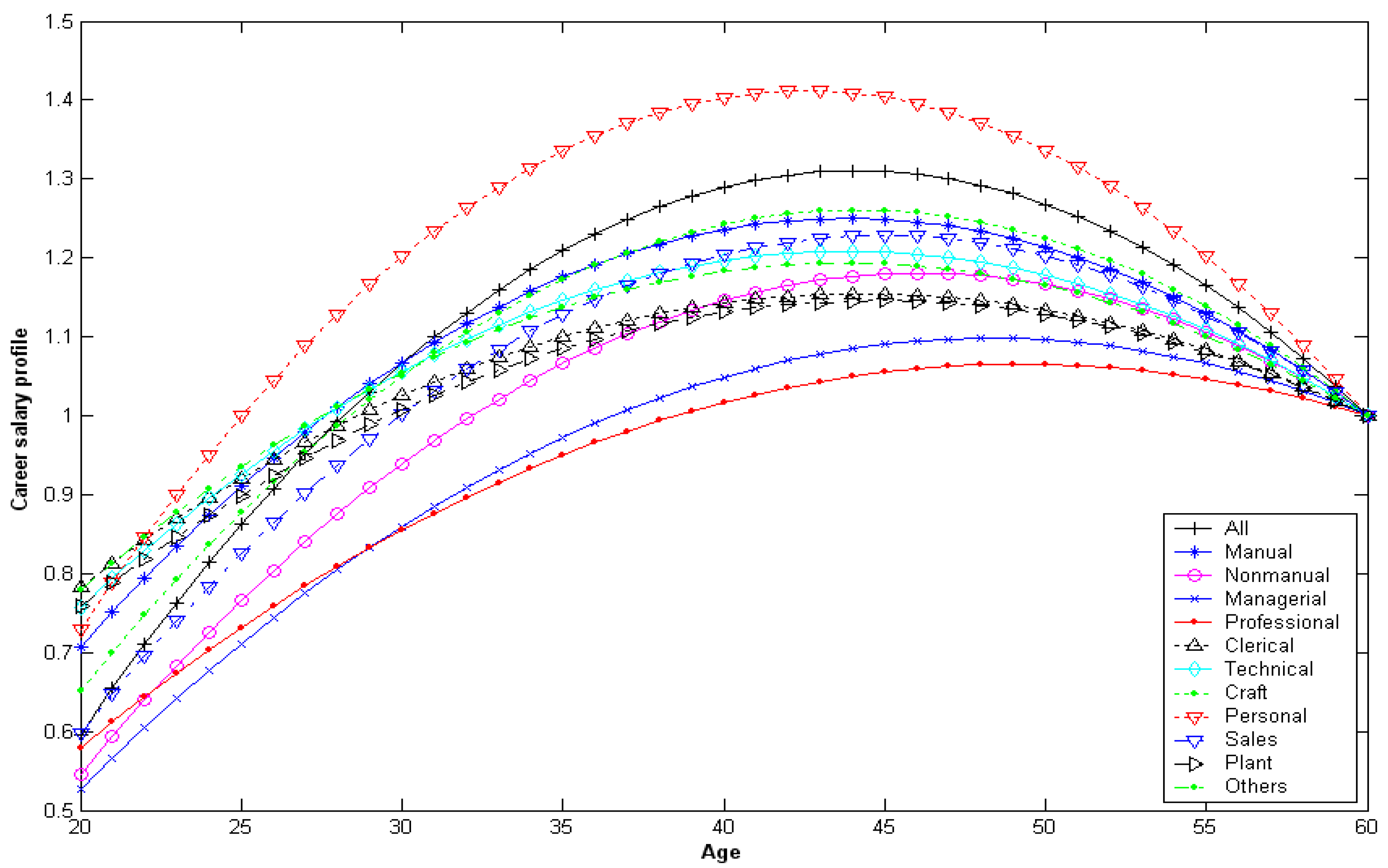
As well as considering member choices, a DC model should also take account of key member characteristics, such as occupation and gender. Occupation is important because of its impact on the career salary profile (CSP)8, i.e., how the member’s salary evolves over his or her working life, and it should be noted that different occupations have different CSPs. Since in DC plans, contributions are generally based on a percentage of annual salary, it is important to know the shape of a member’s CSP in order to project his or her lifetime contributions into the plan. CSPs have a hump-shaped pattern with peak lifetime earnings occurring some time in mid or late career—see Figure 2. The earlier this happens in a person’s the career, the better it is for the retirement pension fund, since peak contributions will be invested for longer. Even within the same occupation, men and women have different shaped CSPs and hence will have different contribution patterns even if they start their careers on the same salary and pay the same contribution rate throughout their career.9 Note that the actual nominal salary received at each age will equal the age point on the CSP plus cumulated wage inflation since age 25, so will not necessarily fall at older ages as steeply as the CSP itself does, if at all.
A further complicating factor is gender in annuity pricing. Traditionally, annuities in the UK and many other countries were priced using annuity tables based on the member’s gender, and this is what we have assumed in our base case. However, since January 2013, insurance companies in the European Union must sell annuities on a gender-neutral or unisex basis. Since the life expectancy of men is lower than that of women of the same age, the effect of this change will be to reduce male pensions and increase female pensions, other things equal. We will illustrate the impact of this change.
Table 3 shows occupation and gender differences in replacement ratios at retirement, assuming the base contribution rate and asset-allocation strategy. The first two lines show that ignoring the CSP can make a big difference to projected retirement replacement ratios: for males, ignoring the CSP leads to an expected retirement replacement ratio of 29.6% using real-gender annuity pricing and 26.7% if we use unisex annuity pricing, whereas assuming the average CSP across all occupations leads to a higher expected retirement replacement ratio of 43.1% for real-gender pricing (and 38.9% for unisex). For females, ignoring the CSP leads to an expected retirement replacement ratio of 24.8% (26.7% for unisex) and taking account of it leads to an expected replacement retirement ratio of 37.1% (40.5% for unisex).
The remaining results presented indicate that there are major differences in expected retirement replacement ratios both across both occupation and gender which will not be captured if the member’s occupation and gender are not modelled. In all cases, the ratios are higher, so ignoring occupation and gender underestimates the attractiveness of DC pensions. Individuals in occupations where the CSP peaks early, such as manual and personal service workers, do relatively well compared with those in occupations where the CSP peaks later, such as managerial and professional workers. In absolute terms, members of the latter group will have higher pensions than the former because they have higher salaries throughout their careers, but they still have lower replacement ratios. We also see, as one would expect, that differences across genders are substantially less with unisex rather than with real-gender annuity pricing. Nevertheless, the results show that even with unisex annuities, the replacement ratios of men and women are not the same since their CSPs differ. For example, male manual workers have a higher replacement ratio than their female counterparts on average because their peak earnings occur at a younger age. The opposite is true for managers.
A good DC model should also be able to handle other member-specific characteristics including, e.g., existing net wealth or debts, and the value of any pre-existing pension fund. The former is important for, say, younger workers with student loans to pay off. The latter is important for older members who might have already accumulated a pension fund and need to periodically reassess their evolving pension prospects as they move towards retirement.
- Principle 6: The model should take account of key member characteristics, such as occupation, gender, and existing assets and liabilities.
The final member characteristic to be considered by the model is attitude to risk, since this determines the member’s allocation to growth and conservative asset classes, as more risk-tolerant members will choose a higher weight in growth assets, while more risk-averse members will choose a higher weight in conservative assets. A good DC model will illustrate the consequences of these decisions in terms of, say, the expected replacement ratio and the 5% VaR as a measure of the downside risk. Knowledge of these consequences might, in turn, influence other plan decisions that the member makes, such as the contribution rate and the planned age of retirement. For example, members who are conservative risk-averse investors might choose to increase the contribution rate and delay retirement. On the other hand, they might find these decisions unpalatable and decide instead that they are not as risk averse as they originally thought and so end up choosing a higher weight to growth assets than they originally indicated. A good DC model will show the consequences of changing asset allocation, contribution rate and planned retirement date, thereby enabling the member to iterate towards his or her preferred combination.10
- Principle 7: The model should illustrate the consequences of the member’s attitude to risk for the plan’s asset allocation decision. It should also show the consequences of changing the asset allocation, contribution rate and planned retirement date, thereby enabling the member to iterate towards the preferred combination of these key decision variables.
6. Modelling Plan Charges
We also need to take account of plan charges, which cover administrative costs and the fund-manager fee. It is important to capture all the charges in the plan, as some plans’ charging structures lack transparency.11
The results in Table 4 show that charges make a considerable difference to retirement pension outcomes. As a rough rule of thumb, each increase of 1 percentage point in the charge leads to a reduction in the expected retirement replacement ratio by about 20%.
There are other potential charges incurred when changing jobs. There might be an exit charge when a member leaves a plan or moves from one plan to another. There might be inactivity charges, i.e., higher charges might be imposed in periods when the member makes no contributions to the pension plan or when the member leaves a plan but keeps the assets in the plan (i.e., becomes a deferred member).12
- Principle 8: The model should take into account the full set of plan charges.
We amend the base case going forward to incorporate an illustrative total charge of 1%.
7. Modelling Longevity Risk
Another factor that should be considered is longevity risk—the impact of typically rising but uncertain future life expectancy. Life expectancy has been rising markedly in recent decades.13 The implication is that a young member will have to take this into account when he or she retires in 40 years’ time or so: annuity factors will be higher and this will reduce the pension at each age compared with someone of the same age retiring today.
Table 5 shows the impact on expected retirement replacement ratios on our base case when one does and does not take account of longevity risk. Ignoring longevity risk, we obtain an expected retirement replacement ratio of 35.1%; taking account of it, we get an expected retirement replacement ratio of 28.9%, i.e., a fall of 17.7% compared with what it would otherwise have been.
As a rough rule of thumb, adding longevity risk leads to an increase in annuity prices of about 30% over a 40-year horizon to age 65, which is equivalent to a fall in replacement ratios of also about 30%; this, in turn, is equivalent to an annual increase in annuity prices or annual decrease in replacement ratios of about 0.75%.
- Principle 9: The model should take account of longevity risk and projected increases in life expectancy over the member’s lifetime.
We amend our base case going forward to incorporate the impact of longevity risk.
8. Modelling the Post-Retirement Period
A good DC model should project post-retirement outcomes as well as at-retirement pension outcomes. This is because at-retirement outcomes may not reflect outcomes later in retirement.
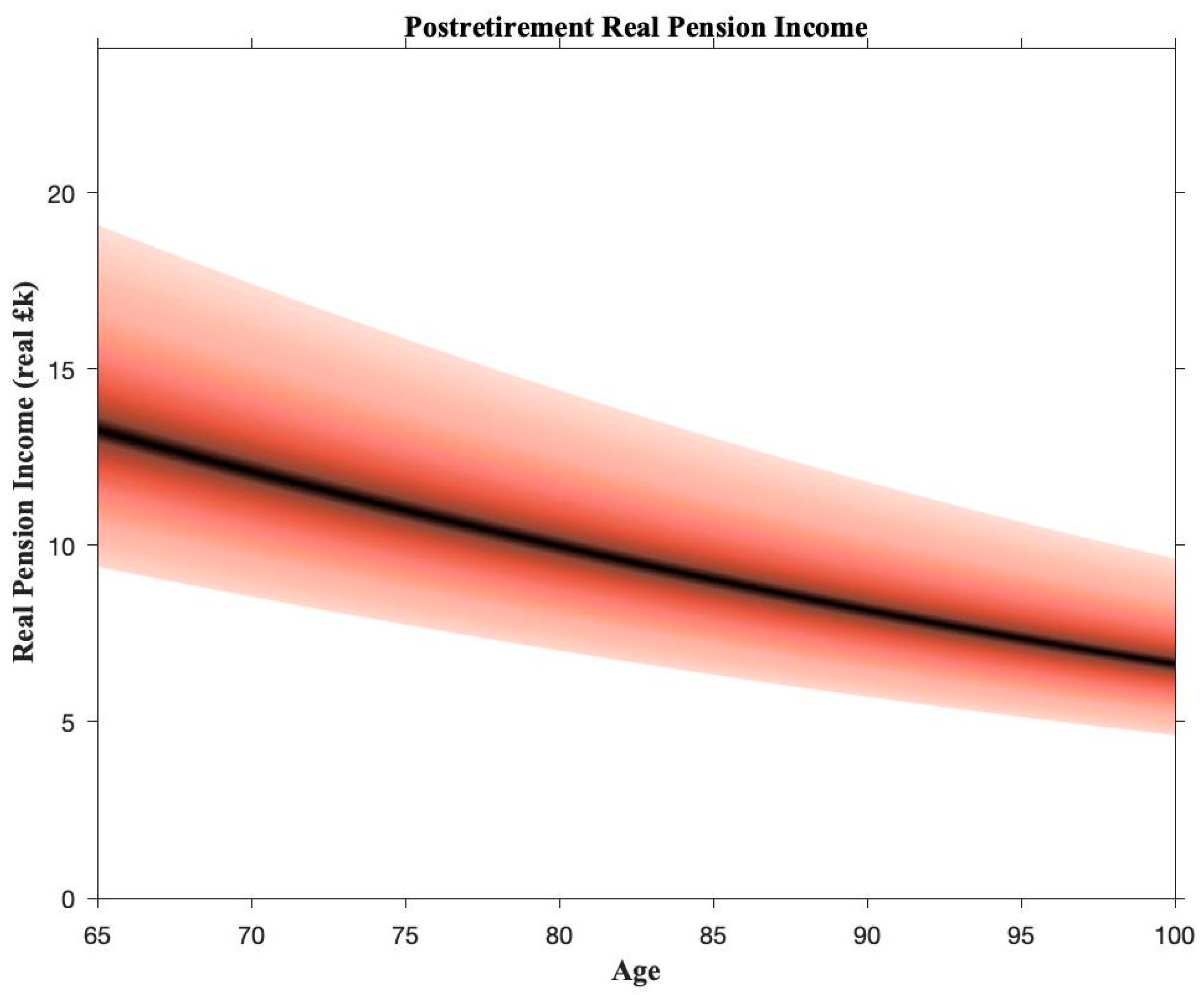
To illustrate this, Figure 3 shows a fan chart for post-retirement real pension income in the case where the member’s decumulation strategy is to convert his pension fund at retirement into a level annuity. However, such an annuity provides no protection against inflation after retirement. Figure 3 shows that even an average inflation rate as low as 2% p.a. causes the member’s real pension income to halve in the period between retirement and his hundredth birthday, assuming he lives that long.
An alternative to conventional annuitisation is index-linked annuitisation, but, as we illustrate in Table 2, index-linked annuities offer a lower initial income than fixed annuities that cost the same amount. A plan member who looks only at the at-retirement outcomes might easily overlook the value of the inflation-protection provided by the index-linked annuity, whose benefit only becomes apparent later in retirement. Eventually, the index-linked annuity will pay out more than the fixed annuity if the member lives long enough.
A second reason for considering the whole post-retirement period is because some decumulation strategies can lead to the member exhausting the fund while still alive.14 For example, if the member chooses a drawdown decumulation strategy, then he or she is effectively living off the pension fund in retirement rather than annuitising it, and, if the drawdown rate is too high in relation to subsequent investment performance—an example would be taking out a fixed amount from the pension fund each year even if the fund’s investments have been performing very badly—the pension fund will be reduced to the point where there is little or nothing left to live off.
- Principle 10: The model should project both at-retirement pension outcomes and post-retirement outcomes. The risks associated with the following strategies should be clearly illustrated:
- The risk of taking a level rather than an index-linked annuity in terms of a reduced standard of living at high ages
- The risk associated with drawdown strategies in terms of taking out more from the fund than is justified by realised investment performance.
9. Integrating Pre- and Post-Retirement Periods
It is important to consider the pre- and post-retirement periods in an integrated way.15 The main reason for this is simple: that unless one looks at both pre- and post-retirement outcomes, it is difficult to determine if the member’s choices are suitable ones in the long run.
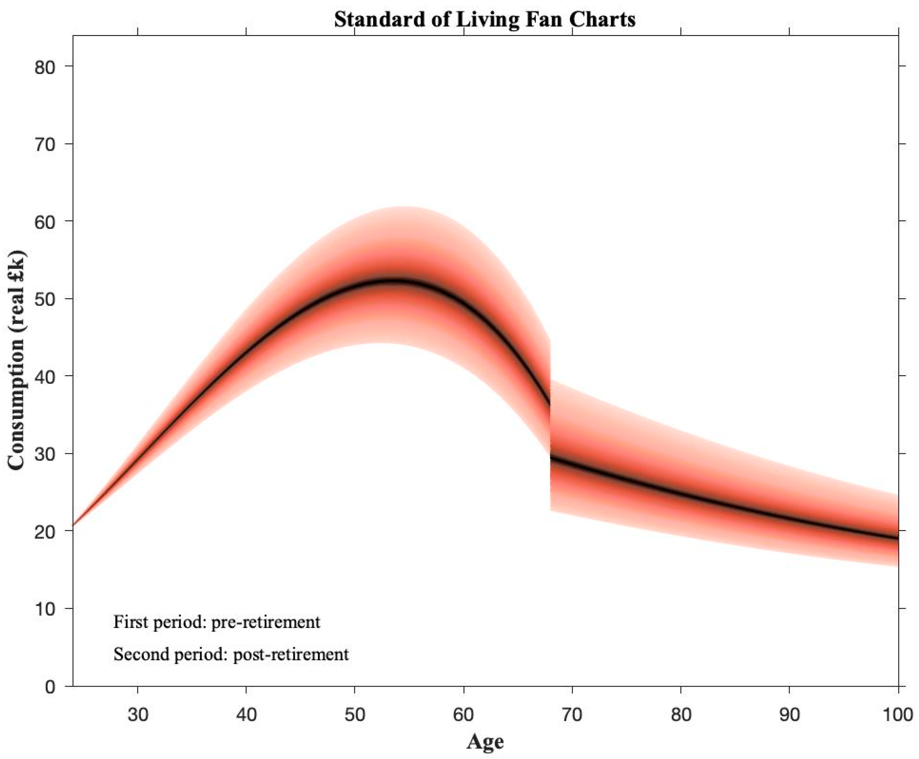
If we look across both pre- and post-retirement periods, there is also a more natural metric than the replacement ratio, which is the levels of pre- and post-retirement standard of living (i.e., the maximum consumption expenditure that is available in each period).
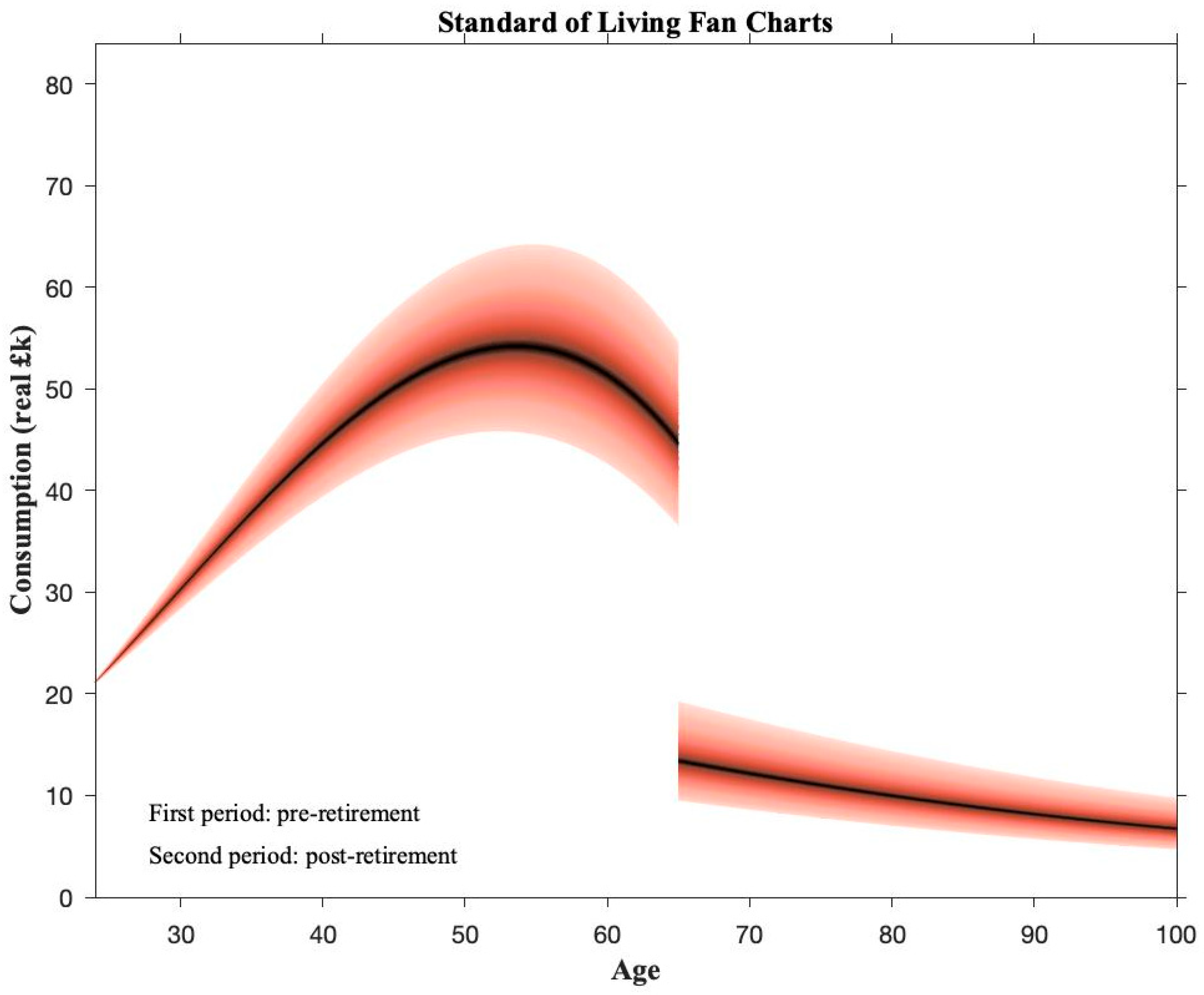
Figure 4 shows standard of living fan charts for both pre- and post-retirement periods for our amended base case. There is a noticeable jump downwards at the point of retirement. People tend not to welcome big cuts in their living standards, so a ‘good’ set of member choices will seek to avoid a big cut at retirement.16 A comparison of standard of living fan charts for alternative sets of choices can be used to guide the member towards their most appropriate set of choices. If the projected fall in retirement consumption is judged to be too high, the member might be encouraged to think in terms of a higher contribution rate, an increased equity weighting, and, perhaps, later retirement.
- Principle 11: The model should consider the pre- and post-retirement periods in an integrated way. This is necessary to avoid undesirable outcomes at a later date—such as a considerable fall in the standard of living in retirement. It will also help to determine what adjustment in member choices—in terms of higher contribution rate, an increased equity weighting and later retirement—are needed to avoid this.
10. Modelling Additional Sources of Income
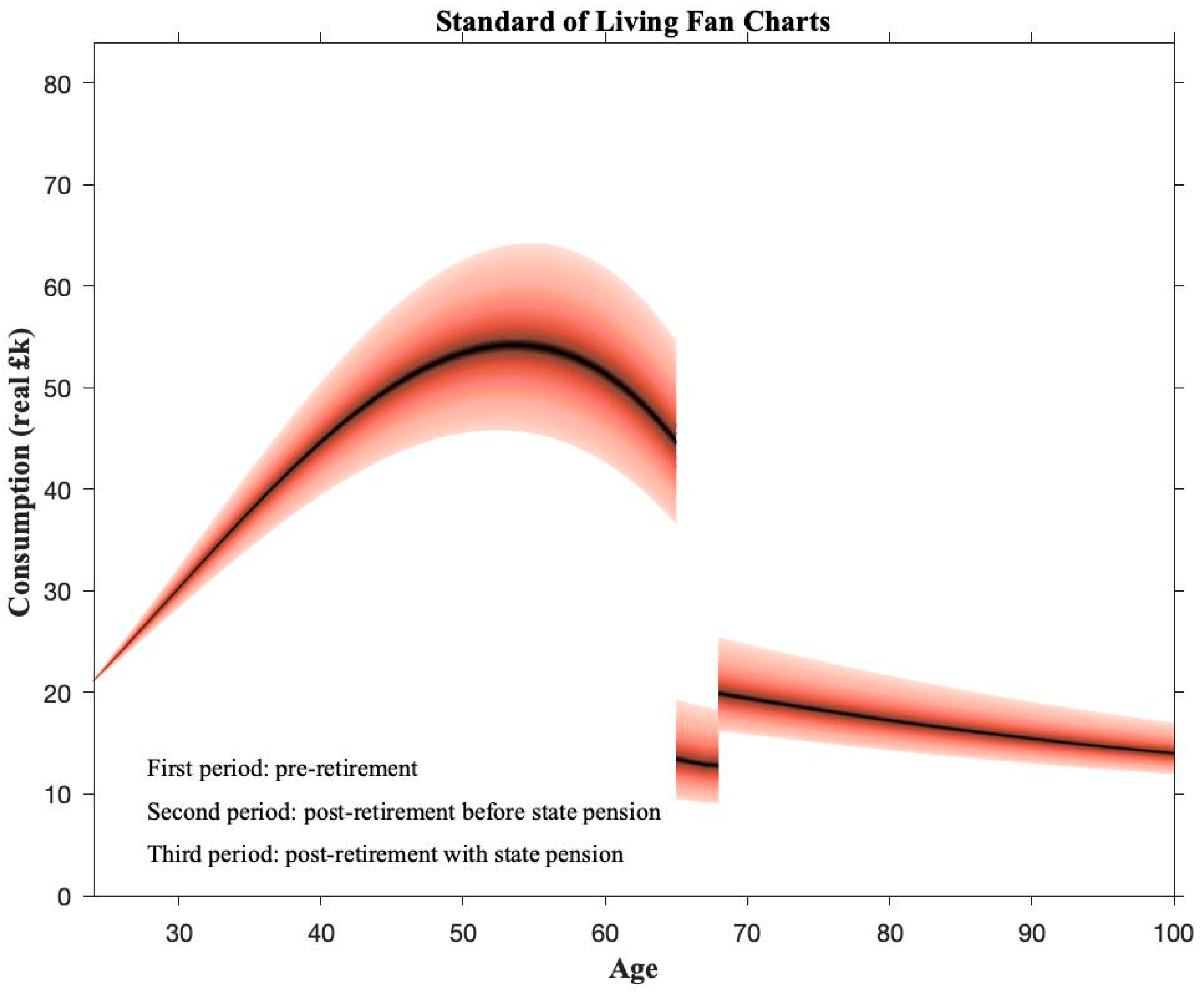
We should also consider other sources of retirement income. One such source is the state pension.17 While it is hard to predict what either the state pension or the state pension age (SPA) will be in 40 years’ time, we can anticipate in the case of the UK that the state pension would be linked to average wages18 and that the SPA might be around 68.19 On the basis of these assumptions, we can add the state pension to our fan chart as in Figure 5. Note how the standard of living rises when the state pension is assumed to begin at age 68. While it is not possible in the UK to receive a state pension before SPA, it is possible to receive a private-sector pension from age 55.20
As an aside, note that the age at which the state pension is received could well differ from the member’s selected retirement age in his DC plan; this is yet another reason why we need to consider outcomes over the range of pre- and post-retirement ages and not just those at the retirement age in the DC plan.
As previously mentioned, any large jumps, such as a substantial fall in retirement at age 65 shown in Figure 4 and Figure 5, are unlikely to be consistent with a ‘good’ set of decisions by the member. The DC model can then be used to guide the member through a decision-making process that leads to outcomes that he or she is comfortable with. Thus, a well-designed DC model will be capable of being a lifetime financial planning tool as well.
There are different ways in which the member might attempt to revise his choices to achieve a smoother consumption profile, but one simple possibility is to increase the contribution rate and delay retirement. For instance, if the member increases his contribution rate from 5% to 8% (so total contributions are 12%) and delays retirement from age 65 to age 68, we can obtain the standard of living fan charts in Figure 6. The consumption profile is much smoother than that in Figure 5, In particular, the big drop previously witnessed at age 65 is now much more attenuated. The initial expected replacement ratio is 54.5%.
- Principle 12: The model should consider other sources of retirement income outside the member’s own pension plan. These include the state pension and home equity release. A well-designed DC model will also help with lifetime financial planning.
We now amend the base case again to incorporate an employee contribution rate of 8% and a SPA of 68.
11. Modelling Extraneous Factors: Unemployment Risk, Activity Rates, Taxes and Entitlements
We have considered the most important factors in DC modelling in the previous sections. Here, we consider some additional factors relating to both the member’s choices and circumstances that again make the modelling process more realistic.
Examples include:
- Unemployment risk
We have assumed so far that the member anticipates working continuously through to retirement, but this ignores the risk of unemployment. When the member is unemployed, he or she is unlikely to continue contributing to his or her pension plan.
- Activity rates
A related issue is the activity rate. The member might be in work but not in full time employment, either voluntarily or involuntarily. If the member is working, say, three days a week, his or her activity rate is 60%. This will influence the contributions going into the pension plan. In this case, we would assume that the member contributes 60% of that of an equivalent member in full time employment.
- Time out of the labour market and resulting skill changes
Some members might deliberately take time out of the labour market. One example might be someone involved in caring for a child or elderly relative. Another example might be someone who spends two years completing an MBA or other qualification. Both examples involve time out of the labour market when there are no earnings and hence no contributions into the pension plan. However, the former might also involve a deterioration in skills, so that when the member returns to work, they are on a lower salary than they would have had had they stayed in work. The latter case will typically involve an enhancement of skills and a higher salary (and possibly even a change of occupation) than had the member stayed in their current job.
- Taxes
For some purposes, the member will need to make decisions that take account of the tax system. This will be the case with pension contributions, where there are tax reliefs to consider, or with wealth management, where the member would want, say, bequests to be made in a tax-efficient manner.
- Welfare entitlements
The model should consider welfare entitlements, such as entitlements to medical care or other support in old age.21
- Principle 13: The model should reflect reality as much as possible and allow for extraneous factors such as unemployment risk, activity rates, taxes and welfare entitlements.
12. Scenario Analysis and Stress Testing
The preceding results are dependent on a range of underlying assumptions. Each set of assumptions constitutes a distinct scenario and we might have economic scenarios, investment return scenarios, mortality scenarios and so forth. It is good practice to consider more than one scenario and to examine how changes in scenarios might affect results. Of particular interest are ‘most likely’ and ‘worst case’ scenarios.22
For any given scenario, one should aim to do the following:
- Make assumptions (especially key assumptions) explicit;
- Evaluate assumptions (especially key assumptions) for plausibility; and
- Stress test assumptions to determine which really matter and which do not. This allows the modeller to determine the important assumptions and focus on getting them (as much as possible) ‘right’.
Our key assumptions include the following:
- Expected nominal wage inflation of 4% p.a.;
- Expected nominal risk-free interest rate of 4% p.a.;
- Expected inflation rate of 2% p.a.;
- Expected nominal return on UK equities of 7.1% p.a.; and
- Standard deviation of the return on UK equites of 18.1% p.a.
To illustrate stress testing, let us stay with our amended base case, but for illustration focus on the replacement ratio at retirement. Table 6 shows the results for a variety of stress tests (which involve a change in one variable, with all other variables held at their mean values), which are:
- A reduction in expected nominal wage inflation from 4% to 3% leads to a rise in the expected replacement ratio at retirement from 54.5% to 66.1%.23
- A reduction in the expected risk-free interest rate from 4% to 3% leads to a fall in the expected replacement ratio at retirement from 54.5% to 48.9%.
- A reduction in the expected inflation rate from 2% to 1% leads to a rise in the expected replacement ratio at retirement from 54.5% to 67.9%.24
- An increase in the expected return on UK equites from 7.1% to 8.1% leads to a rise in the expected replacement ratio at retirement from 54.5% to 67.1%.
- An increase in the standard deviation of the return on UK equites from 18.1% to 19.1% leads to a negligible rise in the expected replacement ratio at retirement from 54.5% to 54.6%, but more significantly leads to a clear widening of the 90% prediction bounds from [35%, 75.6%] to [33.5%, 78.2%].
- Principle 14: Scenario analysis and stress testing are important. For any given scenario, one should also:
- Make key assumptions explicit;
- Evaluate key assumptions for plausibility; and
- Stress test assumptions to determine which really matter and which do not. This allows the modeller to determine the important assumptions and focus on getting them (as much as possible) ‘right’.
13. Periodic Updating of the Model and Changing Assumptions
The model will need to be updated periodically and the assumptions changed. The main reasons for doing so are as follows:
- New or revised information which requires a component of the model to be re-estimated. An example would be the re-estimation of the career salary profiles following the publication a new official survey of salaries by age.
- New or revised information which leads the model builder to change one or more assumptions in order to keep them plausible going forward. Examples here would be the equity premium, the long-term interest rate and the long-term inflation rate.
Such modifications should be carefully documented and explained in order to make sure the model retains its credibility with users. This will help to avoid any subsequent claim that the previous model must have been defective in some way.
- Principle 15: The model will need to be updated periodically and the assumptions changed. Such modifications should be carefully documented and explained in order to make sure the model retains its credibility with users.
14. Fitness for Purpose
Our final modelling principle is that the model should be fit for the purpose to which it is used.25 This is an issue of necessity and sufficiency.
We would argue that the above 15 principles are necessary for a model to be fit for purpose. However, they might not be sufficient. To assess sufficiency, we need to consider how the model is being used, by whom it is being used and for whom it is being used, and we need to do this every time the model is used. Users should also understand the limitations of any model that they use.
We can consider some examples as follows:
- Understandability of the model’s output by the end user. It is important to be aware that a typical member of a pension plan is unlikely to have a strong background in finance and might be overwhelmed by the information from a stochastic model if it is not presented in a manner that can be easily interpreted. For example, whilst the ‘5% value-at-risk’ is likely to be appropriate when considering plan design, it is unlikely to be an appropriate risk metric to communicate to members as it is likely to be unhelpful and confusing.
- Appropriate implementation of the model in a software application. The model must produce output quickly in real time, otherwise the engagement of the end user will be lost. This means that an application that might be suitable as a best-practice design tool for a pension plan might not be a best practice tool for engagement and the provision of retirement financial-outcome information.
- The appropriate focus of the model’s stakeholders. The paper has focused on DC modelling at an individual member level and the importance of ensuring that the modelling sufficiently reflects individual circumstances. However, some model users might have a different focus. For example, some model users might wish to model DC plans on a broader level and so might choose to adopt the above principles, but change the focus to the trustees or providers. This, in turn, would mean that the model user needs to cover a wide spectrum of different member types across different occupations. As another example, the model user might wish to use the model to assess the performance of a fund manager in the accumulation phase by projecting replacement ratios using a combination of the fund manager’s realised returns and the projected returns over the remainder of the accumulation phase based on the fund manager’s agreed benchmark portfolio. This emphasises the importance of all stakeholders framing their discussions and analyses using a common methodology, such as the PensionMetrics methodology.
- Principle 16: The model should be fit for purpose.
15. Attractiveness of the Approach
One of the key attractions of our modelling approach is that we do not require an explicit estimate of the plan member’s risk-aversion or loss-aversion parameter. This is because we have adopted an outcomes-based modelling approach in which the member chooses the pension (or more accurately the range of pension outcomes) he or she desires and the date on which this starts, and this then dictates what the contribution rate and asset allocation needs to be in order to achieve the desired outcome (see, e.g., Blake 2008).
This contrasts with the more common input-based approach which requires an estimate of a risk-aversion or loss-aversion parameter, which is then input into an optimisation routine in order to determine the optimal asset-allocation strategy for the member (see, e.g., Blake et al. 2013, 2014). Although theoretically very appealing, the input-based approach is difficult to implement in practice because of the challenges of determining suitable values of these parameters on the basis of member questionnaires from financial advisers.
In the outcomes-based approach, risk or loss aversion are implicitly reflected in the choice the member makes over the range of pension outcomes. If the member wants to be confident about the level of the pension in retirement, he or she will prefer pension outcomes within a narrow range. This indicates that the member has a high level of risk or loss aversion and, in turn, will accept that he or she will have to make higher contributions and/or to invest in assets with lower volatility and expected returns than a member with a lower level of risk or loss aversion. All of these factors can be assessed by comparing pension outcome or standard of living fan charts. The financial adviser does not need to know the precise value of the member’s risk- or loss-aversion parameter in order to do this.
Another attraction is the visual simplicity of the fan charts in Figure 4, Figure 5 and Figure 6, despite the complexity that underlies them. Financial advisers should find it easy to illustrate different scenarios to a client if they can be produced and compared in real time on a computer or tablet.
16. Conclusions and Caveat
We have set out a methodology to model the quantifiable uncertainty associated with DC pension plans, and have illustrated the model with projections from the PensionMetrics model calibrated to UK data. In doing this, we established 16 good-practice principles in modelling DC pension plans, which are as follows:
- Principle 1: The underlying assumptions in the model should be plausible, transparent and internally consistent.
- Principle 2: The model’s calibrations should be appropriately audited or challenged, and the model’s projections should be subject to backtesting.
- Principle 3: The model must be stochastic and be capable of dealing with quantifiable uncertainty.
- Principle 4: A suitable risk metric should be specified for each output variable of interest, especially one dealing with downside risk. Examples would be the 5% value-at-risk and the 90% prediction interval. These risk metrics should be illustrated graphically using appropriate charts.
- Principle 5: The quantitative consequences of different sets of member choices and actions should be clearly illustrated to help the member make an informed set of decisions.
- Principle 6: The model should take account of key member characteristics, such as occupation, gender, and existing assets and liabilities.
- Principle 7: The model should illustrate the consequences of the member’s attitude to risk for the plan’s asset allocation decision. It should also show the consequences of changing the asset allocation, contribution rate and planned retirement date, thereby enabling the member to iterate towards the preferred combination of these key decision variables.
- Principle 8: The model should take into account the full set of plan charges.
- Principle 9: The model should take account of longevity risk and projected increases in life expectancy over the member’s lifetime.
- Principle 10: The model should project both at-retirement pension outcomes and post-retirement outcomes. The risks associated with the following strategies should be clearly illustrated:
- The risk of taking a level rather than an index-linked annuity in terms of a reduced standard of living at high ages;
- The risk associated with drawdown strategies in terms of taking out more from the fund than is justified by realised investment performance.
- Principle 11: The model should consider the pre- and post-retirement periods in an integrated way. This is necessary to avoid undesirable outcomes at a later date—such as a considerable fall in the standard of living in retirement. It will also help to determine what adjustment in member choices—in terms of higher contribution rate, an increased equity weighting and later retirement—are needed to avoid this.
- Principle 12: The model should consider other sources of retirement income outside the member’s own pension plan. These include the state pension and home equity release. A well-designed DC model will also help with lifetime financial planning.
- Principle 13: The model should reflect reality as much as possible and allow for extraneous factors such as unemployment risk, activity rates, taxes and welfare entitlements.
- Principle 14: Scenario analysis and stress testing are important. For any given scenario, one should also:
- Make key assumptions explicit;
- Evaluate key assumptions for plausibility; and
- Stress test assumptions to determine which really matter and which do not. This allows the modeller to determine the important assumptions and focus on getting them (as much as possible) ‘right’.
- Principle 15: The model will need to be updated periodically and the assumptions changed. Such modifications should be carefully documented and explained in order to ensure the model retains its credibility with users.
- Principle 16: The model should be fit for purpose.
Applying these principles will often have uncomfortable implications for plan members. They will often show that if members want to have a particular standard of living in retirement, then they will be making insufficient contributions to their pension plan, following a recklessly conservative investment strategy, planning to retire too early, or some combination of these. Practitioners have told us that revealing this reality to members might put them off contributing to a pension in the first place. We would argue that it is much better to be realistic about the future than to hide your head in the sand. In addition, there might be pressure to change the assumptions if the outcomes are not liked. This should be resisted, unless there are compelling reasons for doing so.
We would also argue that these principles are fully coherent with the OECD Roadmap for the Good Design of Defined Contribution Pension Plans26 which was published in June 2012, in the following ways:
- Ensuring the design of DC pension plans is internally coherent between the accumulation and payout phases and with the overall pension system: Principles 11 and 12.
- Encouraging people to enrol, to contribute and contribute for long periods: Principle 5.
- Improving the design of incentives to save for retirement, particularly where participation and contributions to DC pension plans are voluntary: Principles 6, 7, 10, 11, 12 and 13.
- Promoting low-cost retirement savings instruments: Principle 8.
- Establishing appropriate default investment strategies, while also providing a choice between investment options with a different risk profile and investment horizon: Principle 7.
- We consider establishing default life-cycle investment strategies as a default option to protect people close to retirement against extreme negative outcomes: Principles 5 and 7.
- For the payout phase, annuitisation as a protection against longevity risk is encouraged: Principle 10.
- Promote the supply of annuities and cost-efficient competition in the annuity market: Principle 10.
- Developing appropriate information and risk-hedging instruments to facilitate dealing with longevity risk: Principle 9.
- Ensuring effective communication and addressing financial illiteracy and lack of awareness: Principles 3–7 and 15.
Furthermore, our principles will be useful in helping providers improve communications in DC pension plans. In January 2013, the European Insurance and Occupational Pensions Authority (EIOPA) published Good Practices on Information Provision for DC Schemes: Enabling Occupational DC Scheme Members to Plan for Retirement.27 The report shows how information can be structured and presented to help plan members make appropriate financial decisions on the basis of the following 10-point checklist:
- Preparation
- Have a behavioural purpose: Principles 5–13.
- Provide a first layer of information that answers key questions of members: Principle 5.
- Ensure information is retrievable.
- Ensure the information provided is comprehensible: Principles 5–13.
- Actual drafting
- 5.
- Optimise attention: Principles 5–13.
- 6.
- Reduce complexity: Principles 7, 10 and 11.
- 7.
- Provide figures that enable personal assessment and understanding: Principles 4, 10 and 11.
- 8.
- Show potential implications of risks and ways to deal with them: Principle 4.
- 9.
- Support readers as much as possible towards financial decisions: Principles 5, 7, 10, 11, 12 and 13.
- Testing
- 10.
- Ensure thorough testing among members.
We end with an important caveat. It relates to the interpretation of the projections considered here: they are not forecasts, but rather stochastic ‘what if?’ projections that indicate the outcomes that might occur if the various underlying assumptions hold true. In other words, they tease out the outcomes implicit in the assumptions. Whether those assumptions later turn out to be true is entirely another matter—and the history of forecasting suggests that all assumptions made about the future are to a greater or lesser extent always false. The experience of the past suggests that the future is always a surprise. This should always be borne in mind when interpreting the output from any DC model.
Author Contributions
Conceptualization, K.D., D.B.; Methodology, K.D., D.B.; Validation, K.D.; Visualization, K.D.; Writing—original draft preparation, K.D.; and Writing—review and editing, D.B. All authors have read and agreed to the published version of the manuscript.
Funding
This research received no external funding.
Institutional Review Board Statement
Not applicable.
Informed Consent Statement
Not applicable.
Data Availability Statement
Data for the age-period-cohort stochastic mortality model were obtained from the Human Mortality Database.
Acknowledgments
The authors have received valuable feedback from David A. Bell (St Davids Rd Advisory), Adam Butt (Australian National University), David Hutchins (AllianceBernstein), Robert Inglis (Financial reporting Council), Andrew Jinks (UK Pensions Regulator), Andrew Storey (eValue) and two anonymous referees.
Conflicts of Interest
The authors declare no conflict of interest.
| 1 | The alternative, defined benefit (DB) plans, are now largely confined to the public sector. |
| 2 | For an example of model backtesting, see Dowd et al. (2010a). |
| 3 | The ratio of the pension at retirement to the final salary before retirement. |
| 4 | This said, the interpretation of any results from DC models should be mindful of unquantifiable uncertainty—the unknown unknowns. The latter by definition always lie beyond the model’s reach, but are ever present and often more important. |
| 5 | They are also subject to revision. For example, they were revised down from 5%, 7% and 9% in April 2014. |
| 6 | A good pension simulation model would also produce density charts for other output variables of interest, such as, pension income or annuity prices (or annuity rates) at retirement. |
| 7 | The annuity factor equals the present value of £1 per annum payable for life from the retirement age until death. If the plan member annuitises the pension in retirement, the annual pension is found by dividing the pension fund by the annuity factor. |
| 8 | Also known as a salary scale. |
| 9 | For more on the career salary profile, see Blake et al. (2007). |
| 10 | Another important member characteristic is risk capacity—that is, the ability to bear risk given the member’s wider circumstances such family commitments, existing debts, age, etc. A member might have the tolerance to take risk, but might not have the capacity to do so. However, risk capacity should be considered in the advice process; it is not something that can be captured in a pension simulation model. |
| 11 | |
| 12 | This charge is known euphemistically in the UK as the loss of the active member discount. |
| 13 | For evidence, see Dowd et al. (2010b). However, increases in life expectancy have slowed down in some countries in recent years (e.g., the US and UK) and we have yet to see the longer-term consequences of the COVID-19 pandemic on future life expectancy trends. All this reinforces the importance of modelling longevity risk. |
| 14 | Some countries have legislation in place which prevents this happening by requiring income to be severely reduced before the fund actually runs out of money. |
| 15 | See, e.g., Blake et al. (2009). |
| 16 | Once people retire, they often do not need as much income to live on as when they were in work—they do not need to pay travel costs to work, for example—so some fall in expenditure after retirement might be acceptable. |
| 17 | Another possible source of retirement income is home equity release or reverse mortgage, i.e., the conversion of the equity in the member’s home (if he or she owns a home) into additional income in retirement. To incorporate equity release, we need to make assumptions about the value of the member’s home, whether he or she already owns the home outright (i.e., has paid off any former mortgage), the type of annuity involved in the transaction (i.e., level vs. index-linked), the age at which the transaction is assumed to take place, and so forth. One typically gets a fairly substantial jump in consumption at the age when the equity release transaction takes effect. |
| 18 | In the UK, the state pension currently increases annually at the higher of wage inflation, price inflation or 2.5%—the so-called ‘triple lock’. Over the long run, we would expect the highest of these to be wage inflation. |
| 19 | The SPA in the UK will increase to 68 between 2044 and 2046; https://www.gov.uk/government/news/second-state-pension-age-review-launches (accessed on 20 January 2022). |
| 20 | https://www.gov.uk/earlyretirement-pension/personal-and-workplace-pensions (accessed on 20 January 2022). |
| 21 | There is a further factor that will become increasingly important in future and that is long-term care. Ideally, pension provision and preparing for the possibility of long-term care should be treated as part of an integrated lifecycle plan. Currently, this is not the case either for most individuals or the state. |
| 22 | |
| 23 | The replacement ratio rises because lower wage inflation reduces the final salary by more than it reduces the value of the pension fund at retirement (and hence the initial pension). |
| 24 | This reflects an increase in real investment returns after inflation. |
| 25 | We received very valuable feedback on an earlier draft of the paper. The feedback could broadly be described as requiring the model to be fit for the purpose for which it is used. We have therefore included an additional modelling principle to accommodate this important insight. We would particularly like to thank David A. Bell, Adam Butt, David Hutchins, Robert Inglis, Andrew Jinks, and Andrew Storey for making this point. We will illustrate this with some examples that our correspondents kindly proposed. |
| 26 | www.oecd.org/finance/private-pensions/50582753.pdf (accessed on 20 January 2022). |
| 27 | https://register.eiopa.europa.eu/Publications/Reports/Report_Good_Practices_Info_for_DC_schemes.pdf (accessed on 20 January 2022). |
References
- Blake, David. 2008. It’s all Back to Front: Critical Issues in the Design of Defined Contribution Pension Plans. In Frontiers in Pensions. Edited by Dirk Broeders, Sylvester Eijffinger and Aerdt Houben. Cheltenham: Edward Elgar, pp. 99–159. [Google Scholar]
- Blake, David. 2014. On the Disclosure of the Costs of Investment Management, Pensions Institute, Discussion Paper PI-1407, May. Available online: http://www.pensions-institute.org/wp-content/uploads/2019/workingpapers/wp1407.pdf (accessed on 20 January 2022).
- Blake, David, and John Board. 2000. Measuring Value Added in the Pensions Industry. Geneva Papers on Risk and Insurance 25: 539–67. [Google Scholar] [CrossRef]
- Blake, David, Andrew J. G. Cairns, and Kevin Dowd. 2001. PensionMetrics: Stochastic Pension Plan Design During the Accumulation Phase. Insurance: Mathematics and Economics 29: 187–215. [Google Scholar] [CrossRef]
- Blake, David, Andrew J. G. Cairns, and Kevin Dowd. 2003. PensionMetrics 2: Stochastic Pension Plan Design During the Distribution Phase. Insurance: Mathematics and Economics 33: 29–47. [Google Scholar] [CrossRef] [Green Version]
- Blake, David, Andrew J. G. Cairns, and Kevin Dowd. 2007. The Impact of Occupation and Gender on Pensions from Defined Contributions Plans. Geneva Papers on Risk and Insurance 32: 458–82. [Google Scholar] [CrossRef] [Green Version]
- Blake, David, Andrew J. G. Cairns, and Kevin Dowd. 2009. Designing a Defined-Contribution Plan: What to Learn from Aircraft Designers. Financial Analysts Journal 65: 37–42. [Google Scholar] [CrossRef]
- Blake, David, Douglas Wright, and Yumeng Zhang. 2013. Target-Driven Investing: Optimal Investment Strategies in Defined Contribution Pension Plans under Loss Aversion. Journal of Economic Dynamics & Control 37: 195–209. [Google Scholar]
- Blake, David, Douglas Wright, and Yumeng Zhang. 2014. Age-Dependent Investing: Optimal Funding and Investment Strategies in Defined Contribution Pension Plans when Members are Rational Life-Cycle Financial Planners. Journal of Economic Dynamics & Control 38: 105–24. [Google Scholar]
- Cox, John C., Jonathan E. Ingersoll Jr., and Stephen A. Ross. 1985. A Theory of the Term Structure of Interest Rates. Econometrica 53: 363–84. [Google Scholar] [CrossRef] [Green Version]
- Dowd, Kevin. 2005. Measuring Market Risk, 2nd ed. Chichester: Wiley. [Google Scholar]
- Dowd, Kevin, Andrew J. G. Cairns, David Blake, Guy D. Coughlan, David Epstein, and Marwa Khalaf-Allah. 2010a. Backtesting Stochastic Mortality Models. North American Actuarial Journal 14: 281–98. [Google Scholar] [CrossRef]
- Dowd, Kevin, David Blake, and Andrew J. G. Cairns. 2010b. Facing up to Uncertain Life Expectancy: The Longevity Fan Charts. Demography 47: 67–78. [Google Scholar] [CrossRef] [PubMed]
- Financial Conduct Authority. 2021. COBS 13 Annex 2 Projections, November 26. Available online: https://www.handbook.fca.org.uk/handbook/COBS/13/Annex2.html (accessed on 20 January 2022).
- Harrison, Debbie, David Blake, and Kevin Dowd. 2012. Caveat Venditor: The Brave New World of Auto-Enrolment Should Be Governed by the Principle of Seller Not Buyer Beware, Pensions Institute, October. Available online: http://www.pensions-institute.org/wp-content/uploads/CaveatVenditor.pdf (accessed on 20 January 2022).
- Hobcraft, John, Jane Menken, and Samuel Preston. 1982. Age, Period and Cohort Effects in Demography: A Review. Population Index 48: 4–43. [Google Scholar] [CrossRef] [PubMed]
Figure 1.
Pension Fund Value and Replacement Ratio at Retirement. Notes: Results in all Figures and Tables are derived from the PensionMetrics model with 10,000 simulation trials. PDF = probability density function. Base case assumptions—Single male joins a DC pension plan at age 25 with a salary of £24,000 which increases in line with the UK ‘average’ career salary profile plus wage inflation. Contributions into the plan are 9% of salary (5% from the employee, 4% from the employer). The investment strategy is 25% in UK equities and 75% in UK government bonds. The member retires at 65 and uses the accumulated pension fund to purchase a single-life level annuity. Expected price and wage inflation are 2% and 4% p.a., respectively, with a standard deviation of 2.5% p.a. each. The nominal risk-free interest rate is 4% p.a., with a standard deviation of 2.5% p.a. The nominal expected returns and standard deviations of the returns are 5.0% and 5.2% p.a. on UK government bonds and 7.1% and 18.1% p.a. on UK equities, respectively. The correlation between the returns on UK government bonds and UK equities is −0.14. The price of the single-life level annuity is based on UK male mortality rates, a discount rate equal to the risk-free interest rate, and a 10% loading factor to cover administration charges and provider profit. Investment returns are modelled using a multivariate Gaussian process and calibrations set out in Harrison et al. (2012), interest and inflation rates are modelled using the Cox-Ingersoll-Ross model (Cox et al. 1985), and mortality rates are modelled using the age-period-cohort stochastic mortality model which originated in Hobcraft et al. (1982).

Figure 2.
Career salary profiles for UK male workers. Notes: Scaled to equal 1 at age 60. ‘All’ is the average CSP over all occupations. Source: Blake et al. (2007, Figure 1).
Figure 2.
Career salary profiles for UK male workers. Notes: Scaled to equal 1 at age 60. ‘All’ is the average CSP over all occupations. Source: Blake et al. (2007, Figure 1).

Figure 3.
Fan Chart for Postretirement Real Pension Income: Decumulation Strategy with a Level Annuity. Notes: The fan chart shows the 90% prediction range for real pension income around the median value indicated by the dark central band, derived from the PensionMetrics model with 10,000 simulation trials. Base-case assumptions—see Notes to Figure 1. Plus annual plan charges of 1% and impact of longevity risk.

Figure 4.
Standard of Living Fan Charts. Note: See Notes to Figure 3.
Figure 4.
Standard of Living Fan Charts. Note: See Notes to Figure 3.

Figure 5.
Standard of Living Fan Charts: State Pension at Age 68. Note: See Notes to Figure 3.
Figure 5.
Standard of Living Fan Charts: State Pension at Age 68. Note: See Notes to Figure 3.

Figure 6.
Standard of Living Fan Charts: Member Contribution Rate 8%, State Pension Age 68 and Member Retirement at Age 68. Note: See Notes to Figure 3. Plus an employee contribution rate of 8% (total contributions of 12%) and a SPA of 68. The initial expected replacement ratio is 54.5%.
Figure 6.
Standard of Living Fan Charts: Member Contribution Rate 8%, State Pension Age 68 and Member Retirement at Age 68. Note: See Notes to Figure 3. Plus an employee contribution rate of 8% (total contributions of 12%) and a SPA of 68. The initial expected replacement ratio is 54.5%.


Table 1.
Illustrative Results for the Replacement Ratio at Retirement (%).
| Lower (5%) Bound | Expected Value | Upper (95%) Bound |
|---|---|---|
| Panel (a): Base case | ||
| 31.0 | 43.1 | 57.8 |
| Panel (b): Increase contribution rate from 9% to 14% | ||
| 52.0 | 73.2 | 96.8 |
| Panel (c): Increase retirement age from 65 to 70 | ||
| 52.2 | 81.5 | 117.0 |
| Panel (d): Decrease retirement age from 65 to 60 | ||
| 18.7 | 25.7 | 33.7 |
Notes: Base case assumptions—see Notes to Figure 1.
Table 2.
Further Illustrative Results for the Replacement Ratio at Retirement (%).
| Lower (5%) Bound | Expected Value | Upper (95%) Bound |
|---|---|---|
| Panel (a): Base case | ||
| 31.0 | 43.1 | 57.8 |
| Panel (b): Increase equity weighting from 25% to 50% | ||
| 28.5 | 47.6 | 72.8 |
| Panel (c): Delay start of contributions from age 25 to age 30 | ||
| 28.2 | 38.4 | 50.9 |
| Panel (d): Index-linked annuity instead of level-annuity | ||
| 26.0 | 36.1 | 48.5 |
| Panel (e): Annuitisation with level joint-life annuity instead of level single-life annuity | ||
| 26.3 | 36.5 | 49.1 |
Notes: Base case assumptions—see Notes to Figure 1.
Table 3.
Occupation and Gender Differences in Replacement Ratios at Retirement (%).
| Occupation | Male | Female | ||
|---|---|---|---|---|
| Real Gender | Unisex | Real Gender | Unisex | |
| Ignore career salary profile | 29.6 | 26.7 | 24.8 | 26.7 |
| Average career salary profile | 43.1 | 38.9 | 37.1 | 40.5 |
| Manual | 40.0 | 36.1 | 30.8 | 33.7 |
| Managerial | 33.4 | 30.1 | 42.7 | 46.6 |
| Professional | 32.0 | 28.9 | 29.1 | 31.8 |
| Clerical | 35.7 | 32.2 | 31.0 | 33.9 |
| Technical | 38.0 | 34.2 | 34.4 | 37.6 |
| Craft | 40.6 | 36.7 | 39.0 | 42.6 |
| Personal services | 47.8 | 43.1 | 32.1 | 35.0 |
| Sales | 39.2 | 35.4 | 31.4 | 34.2 |
| Plant operatives | 35.4 | 31.9 | 29.6 | 32.3 |
| Other | 37.3 | 33.7 | 30.6 | 33.5 |
Table 4.
Charges and Expected Retirement Replacement Ratios.
| Charge (%) | Expected Retirement Replacement Ratio (%) |
|---|---|
| 0 | 43.1 |
| 1 | 35.1 |
| 2 | 28.8 |
| 3 | 23.9 |
Table 5.
Longevity Risk and Expected Retirement Replacement Ratios.
| Expected Retirement Replacement Ratio (%) | |
|---|---|
| No longevity risk | 35.1 |
| With longevity risk | 28.9 |
Notes: Base case assumptions—see Notes to Figure 1. Plus annual plan charges of 1%.
Table 6.
Stress Test Results for the Replacement Rate at Retirement (%).
| Lower (5%) Bound | Expected Value | Upper (95%) Bound |
|---|---|---|
| Panel (a): Base case | ||
| 35.0 | 54.5 | 75.6 |
| Panel (b): Expected wage inflation reduced from 4% to 3% | ||
| 40.6 | 66.1 | 93.9 |
| Panel (c) Expected risk-free interest rate reduced from 4% to 3% | ||
| 31.1 | 48.9 | 67.4 |
| Panel (d): Expected inflation rate reduced from 2% to 1% | ||
| 42.5 | 67.9 | 96.2 |
| Panel (e): Expected return on UK equities increased from 7.1% to 8.1% | ||
| 41.5 | 67.1 | 94.6 |
| Panel (f): Standard deviation of the return on UK equities increased from 18.1% to 19.1% | ||
| 33.5 | 54.6 | 78.2 |
Notes: See Notes to Figure 6.
Publisher’s Note: MDPI stays neutral with regard to jurisdictional claims in published maps and institutional affiliations. |
© 2022 by the authors. Licensee MDPI, Basel, Switzerland. This article is an open access article distributed under the terms and conditions of the Creative Commons Attribution (CC BY) license (https://creativecommons.org/licenses/by/4.0/).
Share and Cite
MDPI and ACS Style
Dowd, K.; Blake, D. Good Practice Principles in Modelling Defined Contribution Pension Plans. J. Risk Financial Manag. 2022, 15, 108. https://0-doi-org.brum.beds.ac.uk/10.3390/jrfm15030108
AMA Style
Dowd K, Blake D. Good Practice Principles in Modelling Defined Contribution Pension Plans. Journal of Risk and Financial Management. 2022; 15(3):108. https://0-doi-org.brum.beds.ac.uk/10.3390/jrfm15030108
Chicago/Turabian StyleDowd, Kevin, and David Blake. 2022. "Good Practice Principles in Modelling Defined Contribution Pension Plans" Journal of Risk and Financial Management 15, no. 3: 108. https://0-doi-org.brum.beds.ac.uk/10.3390/jrfm15030108