Two Types of Payments of Tax on Profit: Advanced Payments and at the End of Periods: Consideration within BFO Theory with Variable Profit

Abstract

Two modifications of a modern theory of capital structure—the Brusov–Filatova–Orekhova (BFO) theory—with variable income are considered: (1) with the income tax payments at the end of periods and (2) with advance income tax payments. BFO formulas for the WACC, and for company capitalization, V, were derived for these two cases. Using the obtained formulas, the dependence of the weighted average cost of capital, WACC; the discount rate; WACC–g (here, g, is the growth rate); company value, V; and the equity cost, ke, on the leverage level, L, at different values of g, at different values of the debt capital cost, kd, and at different values of company age, n, were studied. Comparing the results for cases (1) and (2) shows that case (2) is always preferable for both the company and the regulator. Recommendations have been developed for both parties to expand the practice of advance income tax payments. The managerial implications are as follows. Companies may choose to pay income tax either in advance or at the end of the reporting period in accordance with current results and tax laws. The developed methodology makes it possible to study companies with growing profits and companies with falling profits, which is very important in practice. It also allows the study of companies for which profits could rise and fall in different periods.

1. Introduction

The classical versions of the two main capital structure theories—the Brusov–Filatova–Orekhova (BFO) theory, which is valid for arbitrary age companies, and the Modigliani–Miller (MM) theory, a perpetual version of the BFO theory—are limited to the case of constant profit. But in practice, the profit of the company is, of course, variable. Recently, BFO and MM theories have been generalized for the case of variable profit (Brusov et al. 2021; Brusov and Filatova 2022), which expands significantly the applicability of both theories in practice. In the Brusov–Filatova–Orekhova (BFO) theory, generalized to the case of variable profit (Brusov and Filatova 2022), payments of income tax are made at the end of periods, while, in practice, these payments can be made well in advance. Here, we consider two modifications of the BFO theory with variable profit: (1) with the income tax payments at the end of periods and (2) with advance income tax payments (this case is considered here for the first time). For the above two cases, BFO formulas were derived for WACC, and for the company capitalization, V, and a comprehensive analysis of the dependence of main financial indicators of the company on debt financing at different values of the growth rate, g, at different debt cost values, kd, and at different ages of the company, n, has been conducted. Comparing the results for cases (1) and (2) shows that case (2) is always preferable for both the company and the regulator. Recommendations have been developed for both parties to expand the practice of advance income tax payments. The paper has the following structure.

In Section 1 (Introduction), the formulation of the problem and the novelty of the study are discussed.

In Section 1.1, a review of the literature on capital structure is given.

In Section 2, we consider the modification of the Brusov–Filatova–Orekhova (BFO) theory in the case of companies with variable profit and advance income tax payments. We derive, here, formulas for the value of a financially dependent company, V, for the value of a financially independent company, V₀, for the tax shield value, TS, and for the weighted average cost of capital, WACC. The formulas are derived simultaneously for the following two cases so they made be compared: for income tax payments made at the end of the periods, and for payments made in advance. The latter formula is obtained here for the first time.

In Section 3, we describe the results of the study; the dependences of the WACC; the discount rate; WACC–g; company capitalization, V; and the equity cost, ke, on the debt financing, L, at different values of the growth rate, g, at different values of the debt cost, kd, and at different ages of the companies.

The contribution of the study is as follows: The generalization of the Brusov–Filatova–Orekhova theory for the case of variable income with advance income tax payments is carried out. Within the framework of the obtained generalized BFO formulas for the weighted average cost of capital, WACC, the cost of equity, k_e; the company value, V; the influence of the growth rate, g; the cost of debt, k_d; and the influence of the age of the company, n, on the dependence of the company’s financial indicators on debt financing, were studied. The obtained results are compared with those for the case of payments of income tax at the end of reporting periods. Recommendations were made for both companies and regulators on the payment of income tax.

1.1. A Literature Review

Five stages in the development of the theory of capital structure can be considered from a historical point of view: The first stage (until 1958) is the traditional approach and the second stage (1958–1963) (Modigliani and Miller 1958, 1963, 1966) is associated with the Modigliani–Miller theory, the first quantitative theory of capital structure. From 1964 to 2008 (the third stage), scientists made many modifications to the Modigliani–Miller theory. The fourth stage (2008–2019) is the emergence and development of the Brusov–Filatova–Orekhova (BFO) theory, which removed the main limitation of the Modigliani–Miller (MM) theory associated with the infinite life of the company (Brusov et al. 2018). Finally, the fifth stage (from 2019 to the present), is associated with the adaptation of the BFO and MM theories to the modern financial practice of the functioning of the company, taking into account the real conditions of their work (Brusov et al. 2021; Brusov and Filatova 2022). The traditional approach is based on existing practical experience. From a theoretical point of view, the advantages of debt financing at a low leverage level and its disadvantages at a high leverage level are taken into account, the competition between which forms the optimal capital structure. The optimal capital structure is defined as the level of leverage at which WACC is lowest and company value, V, is highest. There are two versions of the Modigliani–Miller theory: without taxes and with taxes. The following expressions for V, WACC, and k_e take place without taxes:

$$V=V_0=\frac{EBIT}{k_0},$$

(1)

where V₀ is the unlevered company capitalization, EBIT is earnings before interest and taxes, and k₀ is the equity cost at leverage level L = 0.

For WACC, using (1), we obtain

$$WACC=k_0.$$

(2)

From the equation for WACC, we obtain

$$WACC=k_0=k_{\mathrm{e}}{w}_{\mathrm{e}}+k_{\mathrm{d}}{w}_{\mathrm{d}}.$$

(3)

Taking (1) into account, one obtains for the equity cost, k_e,

$$k_{\mathrm{e}}=\frac{k_0}{w_{\mathrm{e}}}-k_{\mathrm{d}}\frac{w_{\mathrm{d}}}{w_{\mathrm{e}}}=\frac{k_0\left(S+D\right)}{S}-k_{\mathrm{d}}\frac{D}{S}=k_0+\left(k_0-k_{\mathrm{d}}\right)\frac{D}{S}=k_0+\left(k_0-k_{\mathrm{d}}\right)L$$

(4)

Here, S is the equity capital value; D is the debt capital value; k_d and w_d are the cost and share of the company’s debt capital; and k_e and w_e are the cost and share of the equity capital. The equity cost increases linearly with the leverage level L (see (4)).

Within the Modigliani–Miller theory with taxes (Modigliani and Miller 1963), the following expression was postulated for the levered company value, V:

$$V=V_0+D\cdot t.$$

(5)

From (5), we obtain for WACC,

$$WACC=k_0\cdot \left(1-w_{d}t\right)$$

(6)

From the definition of WACC, we reach,

$$WACC=k_e\cdot w_e+k_d\cdot w_d\cdot \left(1-t\right)$$

With Formula (6), the following formula for the equity cost, k_e, can be obtained from the Modigliani–Miller theory with taxes,

$$k_e=k_0+L\cdot \left(k_0-k_d\right)\left(1-t\right)$$

(7)

Note that Formulas (7) and (4) (MM with taxes and without taxes) differ by the multiplier (1 − t), which is called “the tax corrector”. It is less than unit, and, thus, the slope of the k_e(L) curve decreases when accounting for taxes.

In (Hamada 1969), the Modigliani–Miller theory was combined with the CAPM (Capital Asset Pricing Model). This took into account both the financial and business risks of the company and was described with the formula below for the company’s leveraged cost of equity, k_e,

$$k_e=k_F+\left(k_M-k_F\right)b_U+\left(k_M-k_F\right)b_U\frac{D}{S}\left(1-T\right),$$

(8)

where b_U is the β–coefficient of the unlevered company. β–coefficient is a measure of systematic risk. It evaluates the tendency of a security’s profitability to move in parallel with the return of the stock market as a whole.

In (Miller 1977), both corporate and individual taxes were taken into account. The following formula for the leveraged value of a company, V, was derived in 1977 by Miller (Miller 1977):

$$V=V_0+\left[1-\frac{\left(1-T_C\right)\left(1-T_S\right)}{\left(1-T_D\right)}\right]\cdot D$$

(9)

where T_S is the tax on income of an individual investor from his ownership of corporation stock, T_C is the tax rate on corporate income, and T_D is the tax rate on interest income from the provision from investors of credits to other investors and companies.

The authors of (Farber et al. 2006; Fernandez 2006; Berk and De Marzo 2017; Harris and Pringle 1985) have formed a more general expression for WACC compared to the one found in the Modigliani–Miller (MM) theory:

$$WACC=k_0\left(1-w_{d}t\right)-k_d{w}_{d}t+k_{TS}t{w}_d$$

(10)

where D stands for the debt value, k₀ stands for the equity cost at zero leverage level, k_d stands for the debt cost, k_TS stands for the tax shield returns, V stands for the levered company value, and VTS stands for the tax shield value.

While the Formula (10) derived in (Berk and De Marzo 2017) is more general than the Modigliani–Miller (MM) one, its use in practical conditions is necessary. The levered company value can be found by discounting the WACC for the unlevered company cash flows in cases when the WACC value is constant over time. For this special case, the formulas could be found in textbooks (Berk and De Marzo 2017; Harris and Pringle 1985).

Because, as it has been suggested by Modigliani and Miller in 1963 (Modigliani and Miller 1963), the debt value, D, is constant, the unlevered company’s expected after–tax cash flow is fixed, and, thus, V₀ is also constant. We can then assume that k_TS = k_d and the tax shield value is TS = tD. Thus, for the levered company value, V, one obtains the ordinary Modigliani–Miller (MM) formula for WACC instead of Formula (10):

$$WACC=k_0\left(1-w_{d}t\right)$$

We believe that the cost of debt, k_d, and the expected return of the tax shield, k_TS, are equal, since both of them are debt-based, and, thus, the “classical” Modigliani–Miller (MM) theory is much more reasonable.

The influence of tax pressure on the financial balance of energy companies was studied in (Batrancea 2021a). As it was shown, tax pressure has a stronger effect on the equilibrium of oil and electricity companies than it does on gas companies. In (Batrancea 2021b), by studying the impact of financial liquidity and solvency on the performance of healthcare companies within the framework of econometric models, it was shown that such financial indicators as the current liquidity ratio, quick ratio, and leverage level significantly affect the performance of the company.

The main limitation of the MM theory—the infinite life of companies and eternal cash flows—was removed in 2008 by Brusov, Filatova, and Orekhova (Brusov et al. 2018), who created the BFO theory, which is valid for companies of any age. A generalization of the valuation of the tax shield, TS, and the company value (unlevered, V₀, and levered, V) was required to modify the MM theory:

$$\begin{array}{l}\mathrm{TS}=k_{\mathrm{d}}DT{\displaystyle \sum _{t=1}^n{\left(1+k_{\mathrm{d}}\right)}^{-t}}=DT\left[1-{\left(1+k_{\mathrm{d}}\right)}^{-n}\right].\\ V_0=\mathrm{CF}\left[1-{\left(1+k_0\right)}^{-n}\right]/k_0;\hspace{1em}V=\mathrm{CF}\left[1-{\left(1+\mathrm{WACC}\right)}^{-n}\right]/\mathrm{WACC}.\\ \frac{1-{\left(1+\mathrm{WACC}\right)}^{-n}}{\mathrm{WACC}}=\frac{1-{\left(1+k_0\right)}^{-n}}{k_0\left[1-{\omega }_{\mathrm{d}}T\left(1-{\left(1+k_{\mathrm{d}}\right)}^{-n}\right)\right]}.\end{array}$$

(11)

Steve Myers (Myers 2001) has derived the following formula for a one-year-old company, which could be obtained easily from Formula (11) by substituting n = 1

$$WACC=k_0-\frac{\left(1+k_0\right)k_{\mathrm{d}}}{1+k_{\mathrm{d}}}{w}_{\mathrm{d}}T$$

while the Modigliani–Miller formula for WACC (Modigliani and Miller 1963) is obtained by substituting $n=\infty$:

$$WACC=k_0\cdot \left(1-w_{d}t\right)$$

The BFO theory is well–known in the literature (for example, see references (Dimitropoulos 2014; Luiz and Cruz 2015; Barbi 2011; Pavel 2018; Franc-Dąbrowska et al. 2021; Angotti et al. 2018; Vergara-Novoa et al. 2018; Mundi et al. 2021; Sadiq et al. 2021; Becker 2022; El-Chaarani et al. 2022; Huang et al. 2020; Islam and Khandaker 2015; Singhal et al. 2022)) and is widely used in practical calculations (see, for example, (Vergara-Novoa et al. 2018; Mundi et al. 2021; Sadiq et al. 2021; Singhal et al. 2022; Brusov et al. 2023)).

1.2. Methods and Materials

We use analytical and numerical methods. We derive analytically (from first principles) all the formulas for the companies’ main financial parameters, and then, using them in Microsoft Excel, calculate the dependence of these parameters on debt financing, L, growth rate, g, cost of debt, k_d, age of the company, n, etc.

2. The BFO Theory for Companies with Variable Profit and Advance Tax on Profit Payments

2.1. The Value of a Financially Dependent Company, V

The BFO theory is generalized below for the first time for the case of variable profit upon advance tax on income payments. We simultaneously consider two modifications of the BFO theory with variable profit: (1) with the income tax payments at the end of periods (formulas with ‘) and (2) with advance income tax payments (this case is considered here) to see the difference in their derivation and in the resulting formulas.

Let us start by deriving the formula for the capitalization of a financially dependent company, assuming that profit for the period grows with the growth rate, g. Note that, below (up to Formula (20)), all derivations for the two cases (1) and (2) are similar; starting from Formula (20), there will be large differences.

Taking into account that the cost of any asset is equal to the sum of discounted values of incomes generated by this asset, one could write for the value of a levered company, V, of age n the following expression:

$$V=\frac{CF}{1+WACC}+\frac{CF\left(1+g\right)}{{\left(1+WACC\right)}^2}+\frac{CF{\left(1+g\right)}^2}{{\left(1+WACC\right)}^3}+\dots +\frac{CF{\left(1+g\right)}^{n-1}}{{\left(1+WACC\right)}^n}$$

(12)

Here, CF is an annual profit of the company. Formula (12) is a geometric progression with denominator

$$g=\frac{\left(1+g\right)}{\left(1+WACC\right)}.$$

(13)

Using (12), we obtain the expression for the value of a levered company, V, of age n:

$$V=\frac{CF}{1+WACC}\cdot \frac{1-{\left(\frac{1+g}{1+WACC}\right)}^n}{1-\frac{1+g}{1+WACC}}=\frac{CF}{WACC-g}\cdot \left(1-{\left(\frac{1+g}{1+WACC}\right)}^n\right)$$

(14)

Using the perpetuity limit ($n\to \infty$), we obtain the following formula for a financially dependent company value, V,

$$V=\frac{CF}{WACC-g}$$

(15)

This formula shows that the discount rate is WACC − g, and not WACC.

2.2. The Value of a Financially Independent Company, V₀

Let us now derive the formula for the value of an unlevered company, assuming that profit for the period grows with the growth rate, g.

$$V_0=\frac{CF}{1+k_0}+\frac{CF\left(1+g\right)}{{\left(1+k_0\right)}^2}+\frac{CF{\left(1+g\right)}^2}{{\left(1+k_0\right)}^3}+\dots +\frac{CF{\left(1+g\right)}^{n-1}}{{\left(1+k_0\right)}^n}$$

(16)

Formula (16) is the geometric progression with denominator

$$g=\frac{\left(1+g\right)}{\left(1+k_0\right)}$$

(17)

Using (16), we obtain the expression for the capitalization for a financially independent company, V, of age n

$$V_0=\frac{CF}{1+k_0}\cdot \frac{1-{\left(\frac{1+g}{1+k_0}\right)}^n}{1-\frac{1+g}{1+k_0}}=\frac{CF}{k_0-g}\cdot \left(1-{\left(\frac{1+g}{1+k_0}\right)}^n\right)$$

(18)

Using the perpetuity limit ($n\to \infty$), we obtain the following formula for a financially independent company value, V₀,

$$V_0=\frac{CF}{k_0-g}.$$

(19)

This formula shows that the discount rate is k₀ − g, and not k₀.

2.3. The Tax Shield Value, TS

Starting from here, formulas for cases (1) and (2) become different (formulas for the payments of income tax at the end of periods are marked with ‘).

The tax shield for n-years in the case of advance payments of tax on profit is equal to

$${\left(TS\right)}_n=t{k}_{d}D+\frac{t{k}_{d}D}{1+k_d}+\dots +\frac{t{k}_{d}D}{{\left(1+k_d\right)}^{n-1}}$$

(20a)

The tax shield for n-years in the case of payments of tax on profit in the ends of periods is equal to

$${\left(TS\right)}_n=\frac{t{k}_{d}D}{1+k_d}+\frac{t{k}_{d}D}{{\left(1+k_d\right)}^2}+\dots +\frac{t{k}_{d}D}{{\left(1+k_d\right)}^n}$$

(20b)

Formula (20) is the geometric progression with denominator

$$g=\frac{1}{\left(1+k_d\right)}$$

(21)

Summarizing (20), one obtains for the tax shield

$${\left(TS\right)}_n=t{k}_{d}D\cdot \frac{1-{\left(1+k_d\right)}^{-n}}{1-\frac{1}{1+k_d}}=Dt\left(1-{\left(1+k_d\right)}^{-n}\right)\cdot \left(1+k_d\right)$$

(22a)

$${\left(TS\right)}_n=\frac{t{k}_{d}D}{1+k_d}\cdot \frac{1-{\left(1+k_d\right)}^{-n}}{1-\frac{1}{1+k_d}}=Dt\left(1-{\left(1+k_d\right)}^{-n}\right)$$

(22b)

$${\left(TS\right)}_n=Dt\left(1-{\left(1+k_d\right)}^{-n}\right)\cdot \left(1+k_d\right)$$

(23)

We obtain, by modifying the first Modigliani–Miller theorem in finite time, the following expression:

$$V=V_0+{\left(TS\right)}_n$$

(24)

Substituting

$$D=w_{d}V$$

(25)

one obtains

$$V\left(1-w_{d}t\left(1-{\left(1+k_d\right)}^{-n}\right)\cdot \left(1+k_d\right)\right)=V_0$$

(26a)

$$V\left(1-w_{d}t\left(1-{\left(1+k_d\right)}^{-n}\right)\right)=V_0$$

(26b)

Substituting into these equations the values of a financially independent company, V₀ (18), and of a financially dependent company, V, (14) one obtains the following expressions:

$$\frac{CF\cdot \left(1-{\left(\frac{1+g}{1+WACC}\right)}^n\right)\cdot \left(1-w_{d}t\left[1-{\left(1+k_d\right)}^{-n}\right]\cdot \left(1+k_d\right)\right)}{WACC-g}=\frac{CF\cdot \left(1-{\left(\frac{1+g}{1+k_0}\right)}^n\right)}{\left(k_0-g\right)}$$

(27a)

$$\frac{CF\cdot \left(1-{\left(\frac{1+g}{1+WACC}\right)}^n\right)\cdot \left(1-w_{d}t\left[1-{\left(1+k_d\right)}^{-n}\right]\right)}{WACC-g}=\frac{CF\cdot \left(1-{\left(\frac{1+g}{1+k_0}\right)}^n\right)}{\left(k_0-g\right)}$$

(27b)

Dividing both parts by $\left(1-w_{d}t\left(1-{\left(1+k_d\right)}^{-n}\right)\cdot \left(1+k_d\right)\right)$,

$$\left(1-w_{d}t\left(1-{\left(1+k_d\right)}^{-n}\right)\right),$$

we obtain the BFO equation for the case of the variable profit of the company

$$\frac{1-{\left(\frac{1+g}{1+WACC}\right)}^n}{WACC-g}=\frac{1-{\left(\frac{1+g}{1+k_0}\right)}^n}{\left(k_0-g\right)\cdot \left(1-w_{d}t\left[1-{\left(1+k_d\right)}^{-n}\right]\cdot \left(1+k_d\right)\right)}.$$

(28a)

$$\frac{1-{\left(\frac{1+g}{1+WACC}\right)}^n}{WACC-g}=\frac{1-{\left(\frac{1+g}{1+k_0}\right)}^n}{\left(k_0-g\right)\cdot \left(1-w_{d}t\left[1-{\left(1+k_d\right)}^{-n}\right]\right)}.$$

(28b)

These two formulas differ with the factor $\left(1+k_d\right)$, which is in the denominator of the right side.

This is the main theoretical result of the current paper.

Using the perpetuity limit ($n\to \infty$), we obtain the following equation for WACC in the Modigliani–Miller theory in the case of variable profit (Brusov et al. 2021)

$$WACC-g=\left(k_0-g\right)\cdot \left(1-w_{d}t\cdot \left(1+k_d\right)\right)$$

(29a)

$$WACC-g=\left(k_0-g\right)\cdot \left(1-w_{d}t\right)$$

(29b)

$$WACC=\left(k_0-g\right)\cdot \left(1-w_{d}t\cdot \left(1+k_d\right)\right)+g$$

(30a)

$$WACC=\left(k_0-g\right)\cdot \left(1-w_{d}t\right)+g$$

(30b)

$$k_e=WACC\left(1+L\right)-L{k}_d\left(1-t\right)$$

(31)

3. Results and Discussions

Below, we describe the results of the study of the dependences of the main financial parameters of the company on the debt financing, L, at different values of the growth rate, g, at different values of the debt cost, kd, and at different company ages. A large database of results for different pairs (k₀, k_d) (k₀ is the equity cost at zero leverage level, L, and k_d is the debt cost) has been created and is available upon request. To illustrate the obtained results and the conclusions, the results for the following typical financial indicators of the five- and ten-year-old companies are presented: k₀ = 0.26; k_d = 0.22; t = 0.2; g = 0.1; 0.05; 0.0; −0.05; CF = 100 (CF is the income per period).

Although the results for the different values of the indicators may be numerically different, the detected qualitative effects are similar.

For both types of payments of tax on profit (at the end of periods (1) and advance payments (2)), as can be seen in Figure 1 for different values of g, all curves WACC(L) start from one point (L = 0; k₀ = 0.26). These curves WACC(L) show the decrease of WACC with leverage level, L, at all g values. The curves WACC(L) increase with the growth rate, g. This is the first manifestation of the fact that under variable income, WACC is no longer a discount rate. As we will see below, the discount rate role has been taken over by WACC–g (here, g is the growth rate).

The five-year company results differ from the perpetual limit—the theory of Modigliani and Miller with variable income results (Brusov et al. 2021). The WACC(L) curves, in the latter case, decrease with the leverage level, L, at g < k₀ and increase at g > k₀. k₀ is the threshold value, g, separating the increasing WACC(L) curves from the decreasing ones, and for g = k₀ WACC = const = k₀. In the first case (the BFO theory), the WACC(L) curves decrease with increasing leverage, L. for all g values. Note that in both the BFO- theory and in the MM- theory the WACC(L) curves increase with the rate g.

As can be seen from Figure 2, the curves (WACC–g)(L) decrease with leverage level, L, at all g values. The curves (WACC–g)(L) decrease with g. Thus, as it will be seen below, the company value, V, will increase with g.

Below, there is an explanation of this behavior of the (WACC–g)(L). All WACC(L) curves originate from the same point (L = 0; WACC = 0.26). The (WACC–g)(L) curves will be ordered as follows for L = 0: the larger the value of g, the lower the starting point, and, hence, the entire graph lies below, that’s why the curves do not intersect. As it will be seen below, the decrease of (WACC–g)(L) with the growth rate, g, will lead to an increase of the company’s capitalization, V, with g.

Now, for each value of g, the two curves (WACC–g)(L), corresponding to two different types of income tax payments ((1) and (2)), start from the same point (k0–g). They are then split into two curves, and the income tax advances correspond to the lower curve. This means that advance income tax payments result in lower WACC–g values for any growth rate, g.

It could be seen from Figure 3 that the company capitalization, V, at fixed g increases with L in the GBFO theory for both types of tax on profit payments: at the end of periods (1) and advance payments (2). The company capitalization, V, increases with g. This is a consequence of a decrease in the discount rate (WACC–g)(L) with an increase of g.

Note that, for each value of g, two V(L) curves corresponding to two different types of income tax payments ((1) and (2)) start from the same point CF/(k₀–g). They are then split into two curves, and the income tax advances correspond to the upper curve. This means that advance payments of income tax result in a higher value for the company, V, at any growth rate, g.

Below, the dependence of the cost of equity, k_e, on leverage level, L, and on growth rate, g, is studied using the GBFO theory at k₀ = 0.26; k_d = 0.22 and g = 0.1; 0.05; 0.0; −0.05, for a five-year company for two types of tax on profit payments: at the end of periods (1) and advance payments (2).

3.1. Calculations of the Equity Cost, k_e

The equity cost, ke, practically linearly grows with leverage level L at all g values (Figure 4). All curves ke(L) start from one point (L = 0; ke = k0 = 0.26). The slope ke(L) grows with g. The slope of all curves, ke(L), corresponding to the income tax payments at the end of periods (1) is greater than that of the curves with advance income tax payments.

Given that the cost of equity capital determines the economically justified amount of dividends, we can draw the following conclusions regarding the dividend policy of the company:

• Higher growth rate, g, justifies higher dividends.
• If a company pays income tax at the end of periods, it must pay large dividends.
• If the company pays income tax in advance, dividends should be lower.

One important remark can be made: when income tax is paid in advance, the dividends paid by the company should be less. In addition, as we saw above, the value of the company in this case is higher. Thus, advance payments on income tax are beneficial to the enterprise.

3.2. Impact of k_d on Financial Indicators

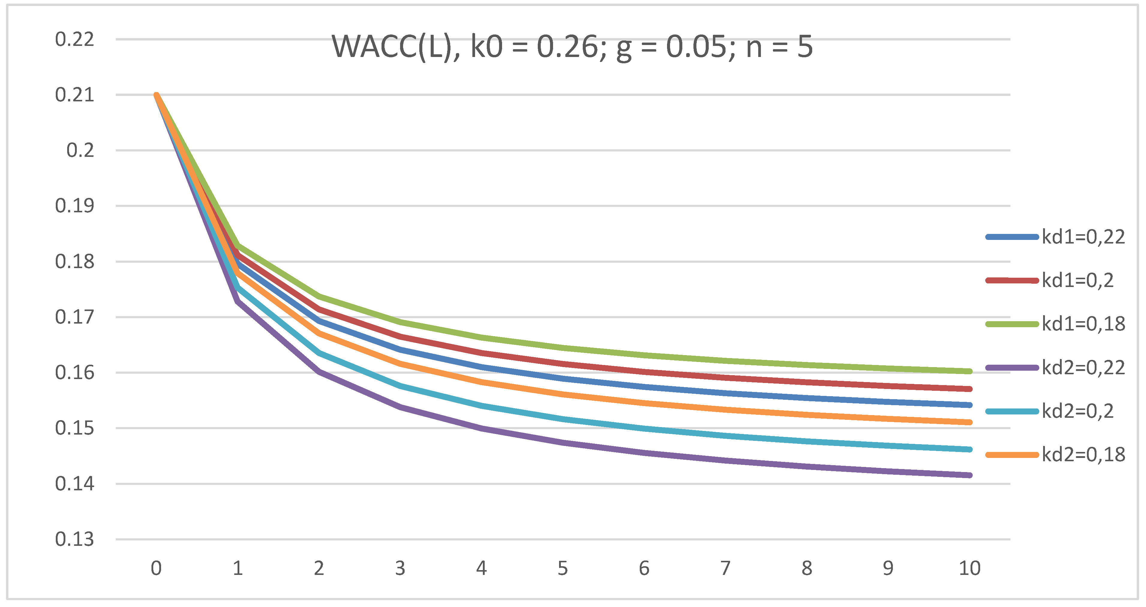
3.2.1. WACC

All curves WACC(L) at all values of k_d start from one point (0; 0.26), as shown in Figure 5. At all values of k_d, WACC(L) decrease with leverage level L and with k_d. All curves WACC(L) in the case of advance income tax payments lie below the curves in the case of income tax payments at the end of periods.

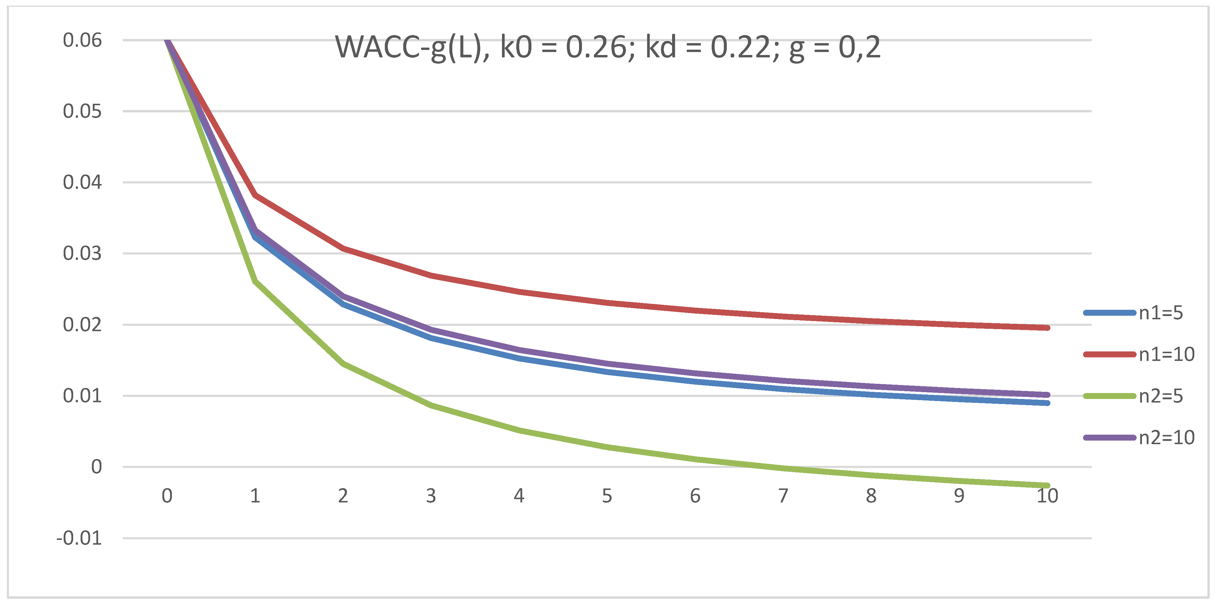
3.2.2. The Discount Rate, WACC–g

All curves (WACC–g) (L) at all values of k_d start from one point (L = 0; k_e = 0.21), as shown in Figure 6. (WACC–g) decreases with L at all values of k_d. (WACC–g)(L) decrease with k_d. This means that the tax shield tends to lower the value of the discount rate (WACC–g) and, hence, (as we will see below in Section 3.2.3) increase the value of the company, V. All curves (WACC–g) (L) in the case of advance income tax payments lie below the curves in the case of income tax payments at the end of periods.

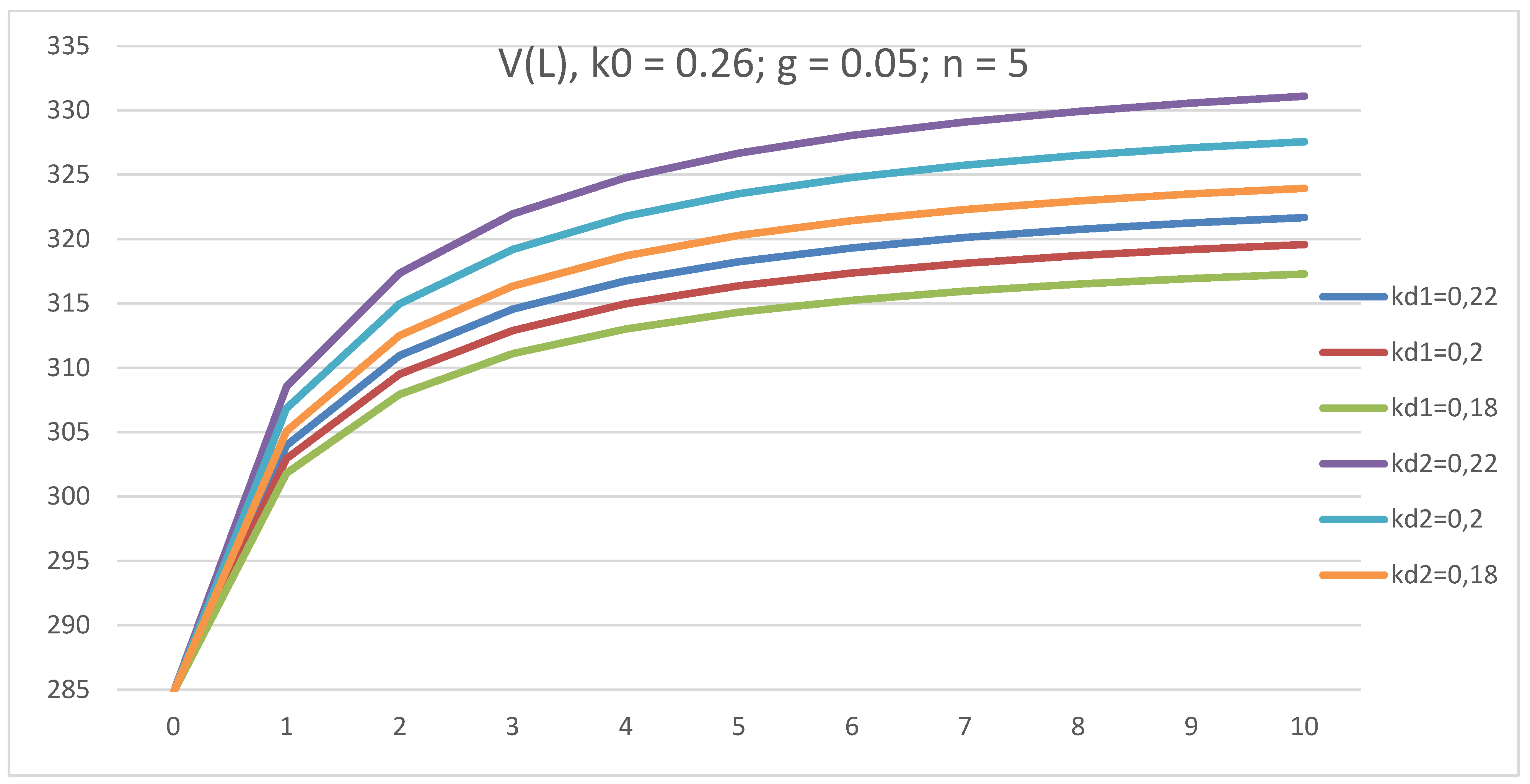
3.2.3. The Company Value, V

All curves of company value, V(L), at all values of k_d for a five-year company start from one point (0; 285), as shown in Figure 7. V(L) increases with L at all values of k_d and V(L) increases with k_d. This means that tax shield advantages increase the company’s capitalization, V. All curves V(L) in the case of advance payments of income tax lie above the curves in the case of the payment of income tax at the end of periods. This means that advance income tax payments are beneficial for the company, as they increase its capitalization.

All curves, ke(L), at all values of k_d start from one point (L = 0; k_e = k₀ = 0.26), as shown in Figure 8, and k_e increases with L at all values of k_d. The slope of ke(L) decreases with the debt cost, kd. Because the equity cost, ke, determines the economically justified amount of dividends, debt cost, kd, impacts the dividend policy of the company. At a fixed cost of debt, kd, the slope of the straight line, ke(L), in the case of income tax payment at the end of the periods is higher than in the case of advance payments.

3.3. Influence of Company Age, n, on Main Financial Parameters of the Company

Below, we study the influence of company age, n, on the main financial parameters of the company. The dependence of WACC; WACC–g; a company’s capitalization, V; and equity cost, ke, on leverage level, L, in the GBFO theory with advance payments of tax on profit at k₀ = 0.26; k_d = 0.22; t = 0.2; g = 0.2; and g = −0.2, for five-year and ten-year companies, is studied. A large difference between the behavior of the company’s main financial parameters with a positive and negative growth rate, g, was found.

3.3.1. WACC(L)

The dependence of WACC on L for companies of two ages (five years old and ten years old) is investigated at g = 0.2 and g = −0.2. In both cases, all WACC(L) curves start from the point (0; 0.26) and decrease with L. WACC is lower for the five-year company for positive g = 0.2, while WACC is lower for the ten-year company for negative g = −0.2. We are seeing this effect for the first time (see Figure 9 and Figure 10).

3.3.2. Discount Rate WACC–g

The dependence of WACC–g on L is investigated for five- and ten-year companies at g = 0.2 and g = −0.2. In both cases, all WACC(L) curves start from one point: (0; 0.06) for g = 0.2 and (0; 0.46) for g = −0.2 and decrease with L. The discount rate, WACC–g, is lower for the five-year company for positive g = 0.2, while WACC–g is lower for the ten-year company for negative g = −0.2. This effect been observed here for the first time (see Figure 11 and Figure 12).

3.3.3. Company Capitalization, V

The dependence of V on L for five- and ten-year-old companies is studied at g = 0.2 and g = −0.2. The capitalization of the company, V, in both cases increases with leverage level, L, and an older age of the company corresponds with a larger capitalization, V. However, if the difference in the value of V for a five-year company and a ten-year company is about 400 at a positive growth rate (g = 0.2), this difference is 45 (ten times less) at a negative growth rate (g = −0.2) (see Figure 13 and Figure 14). Thus, in the competition between the company age and the growth rate, g, the growth rate, g, wins.

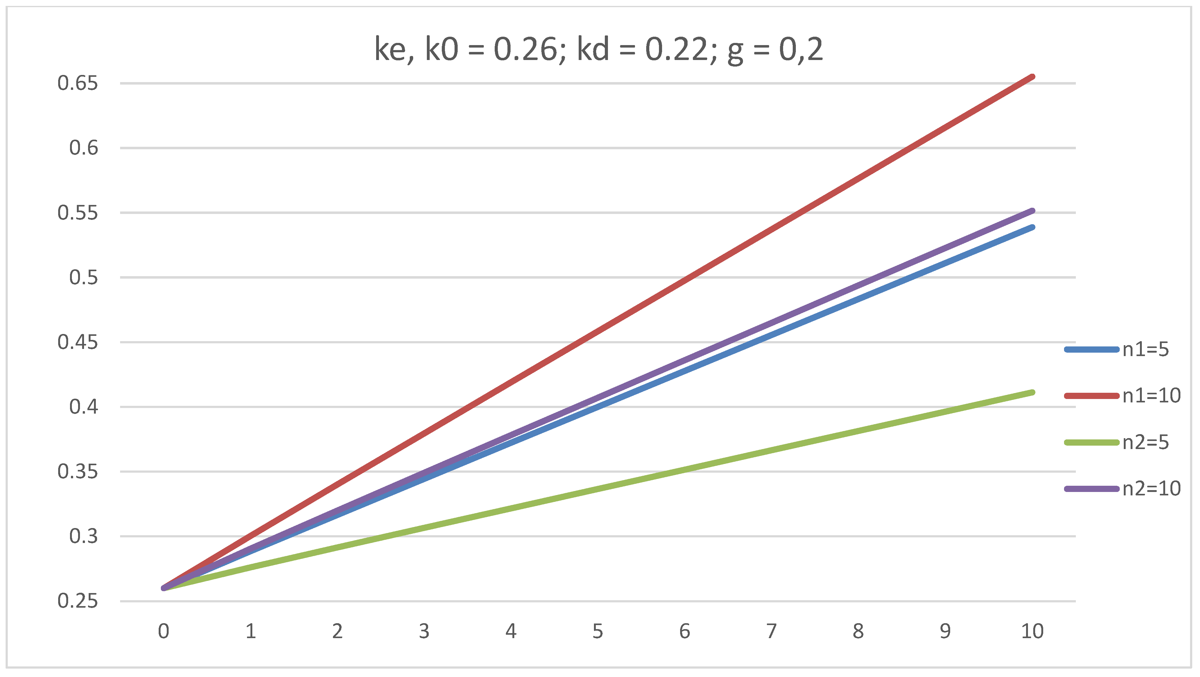
3.3.4. Equity Cost, ke

The dependence of ke on L for five- and ten-year companies is studied at g = 0.2 and g = −0.2. ke increases linearly with L, and the slope of ke(L) for a ten-year company is greater than that of a five-year company in the case of a positive g = 0.2. ke decreases linearly with increasing L, and the negative slope for a ten-year company is greater than that of a five-year company in the case of a negative g = −0.2 (see Figure 15 and Figure 16).

This means that the dividend policy of the company when increasing profits and when decreasing profits should be completely different, because the cost of equity determines the economically justified amount of dividends. This qualitatively new effect has been discovered by us for the first time.

3.3.5. Summary of Results

The curves, (WACC–g)(L), demonstrate the decrease of WACC–g with L at all g. The curves, (WACC–g)(L), decrease with g.

The company’s capitalization, V, increases with L at fixed g in the GBFO theory. The company’s capitalization, V, also increases with g. This corresponds to the decrease of the discount rate (WACC–g)(L) with an increase of g.

The equity cost, ke, practically linearly grows with L at all growth rates, g. The slope ke(L) grows with g.

The influence of k_d on the main financial parameters has been studied and the following results were found:

-

All curves, WACC(L), start from one point (0; 0.26) at all values of k_d. WACC(L) at all values of k_d decrease with leverage level L. WACC(L) decrease with k_d. This means that tax shield leads to the decrease of the cost of raising capital.

-

All curves, (WACC–g)(L), start from one point (0; 0.21) at all values of k_d. At all values of k_d, (WACC–g)(L) decrease with L. With the increase of debt cost, k_d, (WACC–g)(L) decrease. Thus, the tax shield tends to lower the value of the discount rate (WACC–g) and, hence, increase the value of the company, V.

-

At all values of k_d all curves of the company value V(L) start from one point (0; 285) and increases with leverage level L. V(L) increases with k_d. Thus, the tax shield leads to the increase of the company value, V.

-

At all values of k_d, all curves of equity cost, ke(L), start from one point (0; 0.26) and increase with L. The slope of ke(L) decreases with kd. Thus, kd impacts the dividend policy of the company, because ke determines the economically justified amount of dividends.

A huge gap between the behavior of the main financial indicators of the company with a positive and negative growth rate, g, was found.

As seen in

Table 1. Comparison of the results in GBFO theory with payments of tax on profit at the end of periods (1) and advance payments (2) for parameters g (growth rate), k_d (debt cost), and n (company age (for five-year and ten-year companies)) (↑ means an increase in the indicator with the current parameter; ↓ means a decrease in the indicator with the current parameter).

	g Growth Rate		kd Debt Cost		n Company Age			Comparison of (1) and (2)
	Payments at the Ends of Periods (1)	Advance Payments (2)	Payments at the Ends of Periods (1)	Advance Payments (2)		Payments at the Ends of Periods (1)	Advance Payments (2)
WACC	↑	↑	↓	↓	g ≥ 0	↑	↑	1 ≥ 2
					g ≤ 0	↓	↓
WACC–g	↓	↓	↓	↓	g ≥ 0	↑	↑	1 ≥ 2
					g ≤ 0	↓	↓
V	↑	↑	↑	↑	g ≥ 0	↑	↑	1 ≤ 2
					g ≤ 0	↑	↑
ke	↑	↑	↓	↓	g ≥ 0	↑	↑	1 ≤ 2
					g ≤ 0	↓	↓

, the most significant qualitative differences between cases (1) and (2) occur for the dependence of financial indicators on the age of the company. In the cases of the influence of g and k_d, despite the fact that the financial parameters for cases (1) and (2) move in the same direction, there are significant differences between cases (1) and (2) from the quantitative point of view, as well as with respect to the interposition of the financial parameters.

4. Conclusions

We have considered two versions of the Brusov–Filatova–Orekhova (BFO) theory with variable profit for the first time: (1) with the income tax payments at the end of periods and (2) with advance income tax payments. Modified BFO formulas for WACC and for company capitalization, V, were derived for these two cases, and a comprehensive analysis within these formulas of the dependence of WACC; the discount rate; WACC–g; the company value, V; the equity cost, ke; and of the debt financing at different values of the growth rate, g, at different values of the cost of debt capital, kd, and at different values of company age, n, was carried out.

Comparing the results for cases (1) and (2) allowed us to come to the conclusion that case (2) is always preferable for both the company and the regulator. The recommendations for both parties to expand the practice of advance payments of income tax have been developed. The managerial implications are as follows. Companies may choose to pay income tax either in advance or at the end of the reporting period, in accordance with current results and tax laws.

Paper novelties are as follows:

• The generalization of the BFO theory for the case of variable income with advance payments of income tax.
• Generalized BFO formulas for the main financial parameters of the company have been derived.
• Using the obtained formulas, an investigation of the influence of the growth rate, g; the cost of debt, kd; and the company’s age, n, on the dependence of the company’s financial performance on debt financing, has been conducted.
• A comparison of the obtained results with those for the case of paying income tax at the end of the periods has been performed.
• The development of the recommendations for both companies and regulators on how to pay income tax has been created.
• The developed methodology makes it possible to study companies with growing profits and companies with decreasing profits, which is quite important in practice. Regarding the direction of future research, the proposed theory will be used in the future for a more detailed study of companies with both rising and falling profits.

References

1. Angotti, M., R. de Lacerda Moreira, J. Hipólito Bernardes do Nascimento, and O. Neto de Almeida Bispo. 2018. Analysis of an equity investment strategy based on accounting and financial reports in Latin American markets. Reficont 5: 22–40. [Google Scholar]
2. Barbi, Massimiliano. 2011. On the risk-neutral value of debt tax shields. Applied Financial Economics 22: 251–58. [Google Scholar] [CrossRef]
3. Batrancea, Larissa. 2021a. An Econometric Approach Regarding the Impact of Fiscal Pressure on Equilibrium: Evidence from Electricity, Gas and Oil Companies Listed on the New York Stock Exchange. Mathematics 9: 630. [Google Scholar] [CrossRef]
4. Batrancea, Larissa. 2021b. The Influence of Liquidity and Solvency on Performance within the Healthcare Industry: Evidence from Publicly Listed Companies. Mathematics 9: 2231. [Google Scholar] [CrossRef]
5. Becker, Denis Mike. 2022. Getting the valuation formulas right when it comes to annuities. Managerial Finance 48: 470–99. [Google Scholar] [CrossRef]
6. Berk, Jonathan, and Peter De Marzo. 2017. Corporate Finance. Boston: Pearson–Addison Wesley. [Google Scholar]
7. Brusov, Peter, and Tatiana Filatova. 2022. Generalization of the Brusov–Filatova–Orekhova Theory for the Case of Variable Income. Mathematics 10: 3661. [Google Scholar] [CrossRef]
8. Brusov, Peter, Tatiana Filatova, Natali Orekhova, and Mukhadin Eskindarov. 2018. Modern Corporate Finance, Investments, Taxation and Ratings, 2nd ed. Cham: Springer Nature Publishing, pp. 1–571. [Google Scholar]
9. Brusov, Peter, Tatiana Filatova, Natali Orekhova, Veniamin Kulik, She-I. Chang, and George Lin. 2021. Generalization of the Modigliani–Miller Theory for the Case of Variable Profit. Mathematics 9: 1286. [Google Scholar] [CrossRef]
10. Brusov, Peter, Tatiana Filatova, and Veniamin Kulik. 2023. BFO Theory with Variable Profit in Case of Advance Payments of Tax on Profit. Journal of Reviews on Global Economics 12: 1–17. [Google Scholar] [CrossRef]
11. Dimitropoulos, Panagiotis. 2014. Capital structure and corporate governance of soccer clubs: European evidence. Management Research Review 37: 658–78. [Google Scholar] [CrossRef]
12. El-Chaarani, Hani, Rebecca Abraham, and Yahya Skaf. 2022. The Impact of Corporate Governance on the Financial Performance of the Banking Sector in the MENA (Middle Eastern and North African) Region: An Immunity Test of Banks for COVID-19. Journal of Risk and Financial Management 15: 82. [Google Scholar] [CrossRef]
13. Farber, André, Roland L. Gillet, and Ariane Szafarz. 2006. A General Formula for the WACC. International Journal of Business 11: 211–18. [Google Scholar]
14. Fernandez, Pablo. 2006. A General Formula for the WACC: A Comment. International Journal of Business 11: 219. [Google Scholar]
15. Franc-Dąbrowska, Justyna, Magdalena Mądra-Sawicka, and Anna Milewska. 2021. Energy Sector Risk and Cost of Capital Assessment—Companies and Investors Perspective. Energies 14: 1613. [Google Scholar] [CrossRef]
16. Hamada, Robert. 1969. Portfolio Analysis, Market Equilibrium, and Corporate Finance. Journal of Finance 24: 13–31. [Google Scholar] [CrossRef]
17. Harris, Robert S., and John J. Pringle. 1985. Risk-adjusted discount rates-extensions from the average-risk case. Journal of Financial Research 8: 237–44. [Google Scholar] [CrossRef]
18. Huang, Song, Huixia Sun, Huimin Zhao, and Yuening Zhang. 2020. Influence of leverage on the return on equity. Systems Engineering—Theory & Practice 40: 355. [Google Scholar]
19. Islam, Silvia Z., and Sarod Khandaker. 2015. Firm leverage decisions: Does industry matter? The North American Journal of Economics and Finance 31: 94. [Google Scholar] [CrossRef]
20. Luiz, K., and M. Cruz. 2015. The relevance of capital structure on firm performance: A multivariate analysis of publicly traded Brazilian companies. REPeC Brasília 9: 384–401. [Google Scholar]
21. Miller, Merton H. 1977. Debt and taxes. The Journal of Finance 32: 261–75. [Google Scholar]
22. Modigliani, Franco, and Merton H. Miller. 1958. The cost of capital, corporate finance, and the theory of investment. The American Economic Review 48: 261–97. [Google Scholar]
23. Modigliani, Franco, and Merton H. Miller. 1963. Corporate income taxes and the cost of capital: A correction. The American Economic Review 53: 147–75. [Google Scholar]
24. Modigliani, Franco, and Merton H. Miller. 1966. Some estimates of the cost of capital to the electric utility industry 1954–57. American Economic Review 56: 333–91. [Google Scholar]
25. Mundi, Hardeep Singh, Parmjit Kaur, and R. L. N. Murty. 2021. A qualitative inquiry into the capital structure decisions of overconfident finance managers of family-owned businesses in India. Qualitative Research in Financial Markets 14: 357–79. [Google Scholar] [CrossRef]
26. Myers, Stewart C. 2001. Capital structure. Journal of Economic Perspectives 15: 81–102. [Google Scholar] [CrossRef] [Green Version]
27. Pavel, Zhukov. 2018. The Impact of Cash Flows and Weighted Average Cost of Capital to Enterprise Value in the Oil and Gas Sector. Journal of Reviews on Global Economics 7: 138–45. [Google Scholar] [CrossRef]
28. Sadiq, Muhammad, Sami Alajlani, Muhammed Sajjad Hussain, Rashid Ahmad, Furrukh Bashir, and Supat Chupradit. 2021. Impact of credit, liquidity, and systematic risk on financial structure: Comparative investigation from sustainable production. Environmental Science and Pollution Research 29: 20963–75. [Google Scholar] [CrossRef]
29. Singhal, Nikita, Shikha Goyal, Divya Sharma, Sapna Kumari, and Shweta Nagar. 2022. Capitalization and profitability: Applicability of capital theories in BRICS banking sector. Future Business Journal 8: 1–13. [Google Scholar] [CrossRef]
30. Vergara-Novoa, Cristian, Juan Pedro Sepúlveda-Rojas, Miguel D. Alfaro, and Nicolás Riveros. 2018. Cost of Capital Estimation for Highway Concessionaires in Chile. Journal of Advanced Transportation 2153536. [Google Scholar] [CrossRef] [Green Version]
Figure 1. The dependence of WACC on leverage level L GBFO theory with payments of tax on profit at the end of periods (1) and as advance payments (2) at k0 = 0.26; kd = 0.22; t = 0.2; g = 0.1; 0.05; 0.0; −0.05, for a five-year company.
Jrfm 16 00208 g001
Figure 2. The dependence of discount rate, WACC–g, on leverage level, L, in GBFO theory with payments of tax on profit at the end of periods (1) and as advance payments (2) at k0 = 0.26; kd = 0.22; t = 0.2; g = 0.1; 0.05; 0.0; −0.05, for a five-year company.
Jrfm 16 00208 g002
Figure 3. The dependence of discount rate, WACC–g, on leverage level L in GBFO theory with payments of tax on profit at the end of periods (1) and advance payments (2) at k0 = 0.26; kd = 0.22; t = 0.2; g = 0.1; 0.05; 0.0; −0.05, for a five-year company.
Jrfm 16 00208 g003
Figure 4. The dependence of equity cost, ke, on leverage level, L, in GBFO theory with payments of tax on profit at the end of periods (1) and advance payments (2) at k0 = 0.26; kd = 0.22; t = 0.2; g = 0.1; 0.05; 0.0; −0.05 for a five-year company.
Jrfm 16 00208 g004
Figure 5. The dependence of WACC on leverage level, L, in GBFO theory with payments of tax on profit at the end of periods (1) and advance payments (2) at k0 = 0.26; kd = 0.22; 0.2; 0.18 t = 0.2; g = 0.05, for a five-year company.
Jrfm 16 00208 g005
Figure 6. The dependence of discount rate, WACC–g, on leverage level, L, in GBFO theory with payments of tax on profit at the end of periods (1) and advance payments (2) at k0 = 0.26; kd = 0.22; 0.2; 0.18; t = 0.2; g = 0.05, for a five-year company.
Jrfm 16 00208 g006
Figure 7. The dependence of company value, V, on leverage level, L, in GBFO theory with payments of tax on profit at the end of periods (1) and advance payments (2) at k0 = 0.26; kd = 0.22; 0.2; 0.18; t = 0.2; g = 0.05, for a five-year company.
Jrfm 16 00208 g007
Figure 8. The dependence of equity cost, ke, on leverage level L in GBFO theory with payments of tax on profit at the end of periods (1) and advance payments (2) at k0 = 0.26; kd = 0.22; 0.2; 0.18 t = 0.2; g = 0.05, for a five year company.
Jrfm 16 00208 g008
Figure 9. The dependence of WACC on leverage level, L, in GBFO theory with payments of tax on profit at the end of periods (1) and advance payments (2) at k0 = 0.26; kd = 0.22; t = 0.2; g = 0.2, for five-year and ten-year companies.
Jrfm 16 00208 g009
Figure 10. The dependence of WACC on leverage level, L, in GBFO theory with payments of tax on profit at the end of periods (1) and advance payments (2) at k0 = 0.26; kd = 0.22; t = 0.2; g = −0.2, for five-year and ten-year companies.
Jrfm 16 00208 g010
Figure 11. The dependence of discount rate, WACC–g, on leverage level, L, in GBFO theory with payments of tax on profit at the end of periods (1) and advance payments (2) at k0 = 0.26; kd = 0.22; t = 0.2; g = −0.2, for five-year and ten-year companies.
Jrfm 16 00208 g011
Figure 12. The dependence of discount rate, WACC–g, on leverage level, L, in GBFO theory with payments of tax on profit at the ends of periods (1) and advance payments (2) at k0 = 0.26; kd = 0.22; t = 0.2; g = 0.2 for five-year and ten-year companies.
Jrfm 16 00208 g012
Figure 13. The dependence of company value, V, on leverage level, L, in GBFO theory with payments of tax on profit at the end of periods (1) and advance payments (2) at k0 = 0.26; kd = 0.22; t = 0.2; g = −0.2, for five-year and ten-year companies.
Jrfm 16 00208 g013
Figure 14. The dependence of company value, V, on leverage level, L, in GBFO theory with payments of tax on profit at the end of periods (1) and advance payments (2) at k0 = 0.26; kd = 0.22; t = 0.2; g = 0.2, for five-year and ten-year companies.
Jrfm 16 00208 g014
Figure 15. The dependence of equity cost, ke, on leverage level, L, in GBFO theory with payments of tax on profit at the end of periods (1) and advance payments (2) at k0 = 0.26; kd = 0.22; t = 0.2; g = −0.2, for five-year and ten-year companies.
Jrfm 16 00208 g015
Figure 16. The dependence of equity cost, ke, on leverage level, L, in GBFO theory with payments of tax on profit at the end of periods (1) and advance payments (2) at k0 = 0.26; kd = 0.22; t = 0.2; g = 0.2, for five-year and ten-year companies.
Jrfm 16 00208 g016