Deep Learning Approaches for the Mapping of Tree Species Diversity in a Tropical Wetland Using Airborne LiDAR and High-Spatial-Resolution Remote Sensing Images

Abstract

The monitoring of tree species diversity is important for forest or wetland ecosystem service maintenance or resource management. Remote sensing is an efficient alternative to traditional field work to map tree species diversity over large areas. Previous studies have used light detection and ranging (LiDAR) and imaging spectroscopy (hyperspectral or multispectral remote sensing) for species richness prediction. The recent development of very high spatial resolution (VHR) RGB images has enabled detailed characterization of canopies and forest structures. In this study, we developed a three-step workflow for mapping tree species diversity, the aim of which was to increase knowledge of tree species diversity assessment using deep learning in a tropical wetland (Haizhu Wetland) in South China based on VHR-RGB images and LiDAR points. Firstly, individual trees were detected based on a canopy height model (CHM, derived from LiDAR points) by the local-maxima-based method in the FUSION software (Version 3.70, Seattle, USA). Then, tree species at the individual tree level were identified via a patch-based image input method, which cropped the RGB images into small patches (the individually detected trees) based on the tree apexes detected. Three different deep learning methods (i.e., AlexNet, VGG16, and ResNet50) were modified to classify the tree species, as they can make good use of the spatial context information. Finally, four diversity indices, namely, the Margalef richness index, the Shannon–Wiener diversity index, the Simpson diversity index, and the Pielou evenness index, were calculated from the fixed subset with a size of 30 × 30 m for assessment. In the classification phase, VGG16 had the best performance, with an overall accuracy of 73.25% for 18 tree species. Based on the classification results, mapping of tree species diversity showed reasonable agreement with field survey data (R²_Margalef = 0.4562, root-mean-square error RMSE_Margalef = 0.5629; R²_{Shannon–Wiener} = 0.7948, RMSE_{Shannon–Wiener} = 0.7202; R²_Simpson = 0.7907, RMSE_Simpson = 0.1038; and R²_Pielou = 0.5875, RMSE_Pielou = 0.3053). While challenges remain for individual tree detection and species classification, the deep-learning-based solution shows potential for mapping tree species diversity.

1. Introduction

There is much evidence to support the importance of tree species diversity for maintaining wetland ecosystems, according to Schäfer et al. [1]. With the ongoing loss of biodiversity, mapping tree species diversity can provide valuable insights for ecologists [2] and is also essential from the perspective of environmental monitoring and conservation management [3]. Traditional biodiversity measurement is often conducted by field work or monitoring systems [4]. However, these means cannot provide spatially distributed and updated information [5]. Remote sensing techniques can solve this problem and have been used for biodiversity monitoring, as they can cover large areas of multiple spatial scales [6,7,8,9].

Hyperspectral remote sensing imaging, or imaging spectroscopy, has been widely utilized in measuring biodiversity distribution due to its significant capacity for spectral measurement in identifying species [10,11]. Zhao et al. [12] used a species-driven leaf optical trait method called “spectranomics” for forest species diversity mapping. They identified interspecies variations in terms of biochemical and structural properties from airborne hyperspectral images. In their approach, a maximum number of 13 species could be identified. They also reported that their methods would be limited in other areas, as the algorithm would reach saturation when the species richness is high. Previous studies also explored supervised classification methods for tree species discrimination. Yang et al. [13] conducted mangrove species mapping based on AISA+ hyperspectral imagery. A minimum noise fraction transformation was employed for spectral dimensionality reduction. Classification approaches such as maximum likelihood (ML) and spectral angle mapper (SAM) were used for tree species distinguishing, and ML showed good capabilities in their study. Nevalainen et al. [14] employed k-nearest neighbors (k-NN), naive Bayes, decision trees C 4.5, multilayer perceptron (MLP), and random forest (RF) for five tree species classification in southern Finland, and they investigated different feature compositions for the input. Dalponte et al. [15] analyzed multisensor images for tree species identification, and different data setups were fed to supervised classifiers, such as support vector machine (SVM) and RF classifiers. They reported that the multispectral data performed worse compared with the hyperspectral images and high-density light detection and ranging (LiDAR) data, and a similar conclusion was drawn by Goodenough et al. [16].

Isolating individual trees from remote sensing images has been found to be beneficial for tree species diversity mapping [1,17], as the within-class spectral variation can be reduced over the individual tree crowns. However, plant-level mapping is constrained when an individual tree is smaller than the spatial resolution of remote sensing images [18]. Recently, very high spatial resolution (VHR) images with low spectral resolution have found to be able to provide a detailed spatial distribution of tree species types, which enables individual tree detection. Getzin et al. [19] proposed a multiregression approach using the canopy gaps derived from VHR unmanned aerial vehicle (UAV) images for biodiversity assessments in forests and demonstrated the potential of cost-effective VHR images in biodiversity mapping. Despite that studies have exploited VHR data for forest–nonforest classification or coniferous–broadleaf classification [20,21,22], it remains a challenge to use VHR images for tree species identification [15]. A number of studies have utilized pixel-wise classification based on the spectra of leaves but have largely ignored the texture information of tree canopies (a visual feature that contains information on the structure arrangement of the trees in an image and their relationship with neighbors). To allow for possible identification of tree species using VHR images, there is a need to exploit detailed spatial information, such as shape, texture, and context information. To overcome the abovementioned difficulties, many studies developed object-based methods that segment homogeneous and adjacent pixels into objects [23,24]. Object-based classification can make better use of features, such as shape or texture, than the pixel-wise classification, but the determination of the object size is difficult across complex scenes.

Deep learning approaches have become powerful tools for feature extraction and image processing in computer vision [25] and even in remote sensing [26,27]. Deep learning approaches have proved to be superior to traditional machine learning methods in a number of remote sensing applications. In their review, Ma et al. [26] showed that nearly 200 publications using deep convolutional neural networks (CNNs) have been published in the field of remote sensing by early 2019 of which most focused on land use land cover (LULC) classification [28], urban feature extraction [29,30,31], and crop detection [32,33]. Deep learning approaches often require a large amount of training data, and there are benchmark datasets publicly available for training and testing of deep learning approaches in the abovementioned remote sensing fields. Compared with the studies mentioned above, very few studies using deep learning have focused on trees or forest classification [34]. Flood et al. [35] used a U-net convolutional neural network to extract woody vegetation extent from high-resolution three-band Earth-I imagery. In their research, a selection of 1 km² was manually labeled for training. The final results were pixel-wise and only two types (trees and large shrubs) were mapped. If there are diverse tree species, pixel-wise data labeling will be difficult and costly, especially in forested areas. Li et al. [36] proposed a deep-learning-based approach for detecting and counting oil palm trees. In their research, the simple deep learning model of LeNet was used as the classifier and the model input was determined by a sliding window size of 17 × 17 pixels. The sliding step was found to have large impacts on the detection results, the palm trees could be repeatedly detected or missed if the sliding window size was too small or large, respectively. Compared with pixel-based tree species classification, patch-based tree samples can better extract useful spatial context features for classification. In this study, we aimed to evaluate the potential of deep learning to classify tree species at the individual tree level by using airborne LiDAR and high-spatial-resolution aerial images for the purpose of diversity mapping. To achieve this goal, (1) individual trees were first identified using LiDAR data, and the tree apexes were distinguished. The tree patches were then cropped based on the detected tree apexes and three-band VHR images. (2) The training and test samples of 17 tree species and one class named “Others” were surveyed in the field work. The samples were labeled at the individual tree level, and three deep CNNs were modified for tree species classification. (3) Tree species diversity was mapped based on the individual tree species. A tropical wetland named Haizhu Wetland in South China was selected as the study area.

2. Study Area and Materials

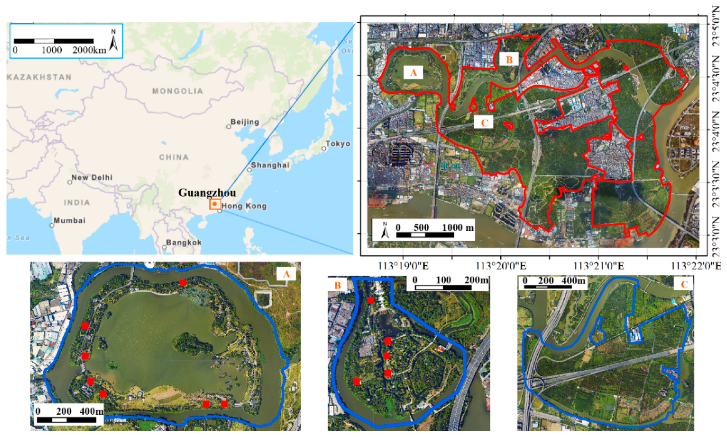
2.1. Study Area

The Haizhu National Wetland Park (centered at 23°04′7.06″N, 113°20′2.30″E) is located in the city of Guangzhou in Guangdong Province in South China. This wetland covers approximately 869 ha (377 ha are water area), with an elevation range of −1 to 9 m above sea level. It is a composite wetland ecosystem of the Pearl River Delta, inland lake wetland, and orchard, but it also contains land cover types such as roads, water, and buildings. It is also an important ecological barrier in South Guangzhou. The Haizhu National Wetland Park consists of three parts (marked A–C in Figure 1). Area A is also referred to as Haizhu Lake Park, and a forest (dominant by broadleaved trees) grows along the lake. Area B is a semiconstructed wetland mixed with various broadleaved trees, including flowering and fruit trees. Area C is mainly covered by neatly arranged fruit trees. On the basis of the original orchard, tree species enrichment and habitat restoration have been conducted for the Haizhu National Wetland in the past few years, making it a good ecological environment for birds. The forest across Haizhu National Wetland Park is now heterogeneous with approximately 20 dominant tree species, including evergreen broadleaved species (such as Ficus microcarpa Linn. f., Delonix regia, and Chorisia speciosa A.St.-Hil) and fruit trees (such as longan and litchi). Here, we selected all of Area A and parts of Areas B and C as the study area (Figure 1).

2.2. Field Survey

The field work was conducted in June 2018 and March and May 2019. Twelve square plots with the size of 30 × 30 m were randomly surveyed across the Haizhu National Wetland, covering the dominant tree species. We also collected single-tree samples for the dominant tree species, including the broadleaved tree species (banyan tree (F. microcarpa Linn. f.), flame tree (D. regia), silk floss tree (C. speciosa A.St.-Hil.), Bauhinia (Bauhinia purpurea Linn.), eucalyptus trees (Eucalyptus robusta Smith), sakura tree (Cerasus sp.), pond cypress (Taxodium ascendens Brongn), Alstonia scholaris, Bischofia javanica Bl., Hibiscus tiliaceus Linn., and camphor tree (Cinnamomum camphora (L.) Presl.)) and the fruit tree species (litchi (Litchi chinensis Sonn.), longan (Dimocarpus longan Lour.), banana (Musa nana Lour.), papaya (Carica papaya), carambola (Averrhoa carambola L.), and mango tree (Mangifera indica L.)). The plots as well as the single-tree samples were positioned by the Guangzhou Continuous Operating Reference System (GZCORS) and Electronic Total Station. The trees with a diameter at breast height (DBH) larger than 5 cm were measured, and the corresponding tree species were recorded. Finally, a total of 2439 scattered trees and 304 trees in 12 plots (the red squares in Figure 1) were surveyed for 17 dominant species and one class of nondominant tree species.

2.3. Remotely Sensed Data

The remotely sensed data we used were high-resolution RGB images and LiDAR point clouds, which were acquired in September 2017 over the research site. A Trimble Harrier 68i laser scanner and a frame amplitude aero digital camera were mounted on a Yun5 airplane for data collection, and the flight height was about 1000 m. The RGB images in Tiff format were orthorectified by ground control points and mosaicked, while the LiDAR point clouds were stored in LAS format. These aerial data were collected with good and similar weather conditions as well as atmosphere transparency, which can be considered in the approximate imaging conditions. The ground sampling distance of RGB images was 0.1 m, and there were five to eight LiDAR points per square meter. The point clouds were firstly preprocessed to remove the noisy values. Digital surface models (DSMs) and digital elevation models (DEMs) were derived using the raster conversion and filtering in LAS tools with a spatial resolution of 0.1 m. A canopy height model (CHM) was created to obtain the height of trees by subtracting DEM from DSM for further individual tree detection.

3. Methodology

3.1. Overview

Unlike traditional tree species classification methods that predict the tree species class label per pixel or per segmented object, our method was designed to infer patch-level prediction. As shown in Figure 2, the training and test samples were in the form of image patches rather than pixels or objects, and finally, each image path was assigned a label of tree species. Figure 2 presents the flowchart of our method with three major steps. Firstly, the individual trees (the information of tree location with x and y coordinates) were isolated based on the CHM via a local maxima algorithm [37]. The individual tree patches were then cropped according to the tree apexes and RGB images. Secondly, three deep learning methods (i.e., AlexNet, VGG16, and ResNet50) were modified for tree species classification. The cropped tree image patches were fed into the CNNs, and finally, 17 dominant tree species and a class of “Others” were identified. Lastly, we performed tree species diversity mapping based on the results of individual tree detection and tree species classification, and the diversity indices, namely, the Margalef richness index, the Simpson diversity index, the Shannon–Wiener diversity index, and the Pielou evenness index 1, and species richness were calculated for the three parts of the Haizhu Wetland. The diversity mapping results were assessed based on the 12 field-surveyed plots.

3.2. Individual Tree Detection

Individual tree detection is an important procedure for further species diversity mapping. In this study, individual trees were detected based on the CHM (in the format of dtm derived from LiDAR point clouds) by the local-maxima-based method (CanpyMaxima, Popescu et al. [37]) in the FUSION software (Version 3.70, Seattle, USA). The height thresholds were set as 1.8–3 m, which varied from different stands. The individual trees were detected and output in the format of a CSV file in which the information of tree location (x and y coordinates), tree height, crown width, and height to crown base were recorded. As there were artificial structures in the research site, points on the buildings or other structures were removed based on the nonvegetation mask. The 12 plots surveyed in the field work were used for individual tree detection assessment.

The individual tree image patches were obtained for further tree species classification based on the detected tree locations (the x and y coordinates of the tree apexes) and the RGB images over the research site. The treetops, which were in the format of points, could be overlaid on the RGB image. Centered on the treetops, we cropped the RGB image into image patches (individual trees), each of 64 × 64 pixels (Figure 3).

3.3. Deep Learning Methods for Tree Species Classification

In the past few years, CNNs have been a hot topic in the field of image classification. Since the publication of AlexNet [38], a number of classical CNN architectures have been proposed, including VGG [39], GoogLeNet [40], and ResNet [41]. VGG can be considered as a deepened version of AlexNet, which employed small convolutional kernels. GoogLeNet adopted the Inception module, which is easy to use for network modification. It also removed the fully connected layers to reduce the number of parameters. Moreover, it used two auxiliary classifiers to accelerate network convergence. As a consequence of the auxiliary classifiers, GoogLeNet is not as scalable as VGG. On the other hand, the depth of networks is a crucial factor that influences CNN performance [39]. Richer features of different levels can be extracted from deep CNN layers, whereas deep models are not easy to optimize. In many studies, batch normalization (BN) is employed to hamper vanishing/exploding gradients in deep CNNs. However, the accuracy often becomes saturated and then degrades (degradation problem) in the training phase, even though BN layers are used. ResNet [41] addressed the degradation problem by using shallow layers and identity mapping for network construction. Two shortcuts (i.e., identity and projection shortcuts) have been introduced for residual learning. Recently, these networks have been introduced into the field of remote sensing.

Our tree species classification strategy takes advantage of recent CNNs for patch-wise classification. We formulated the tree species classification as a supervised image classification problem to identify 18 tree species (17 dominant trees species and a class of “Others”). For this purpose, we adopted AlexNet, VGG16, and ResNet50 implemented in Caffe for individual tree classification. Some adaptive modifications were made for our tree classification problem: (1) The input image size was modified and set as 64 × 64 pixels instead of the original size of each convolutional neural network. (2) The corresponding convolutional and pooling layers were adjusted for feature extraction accordingly. (3) The final output layers were also modified to 18 classes, so as to distinguish 17 dominant tree species and the class of “Others”. The detailed architectures of the three CNNs are shown in Figure 4. In the procedure of our deep-learning-based tree species classification, both training and test data were image patches of individual tress.

To avoid the distinction of identical textures only differing from each other by orientation changes and to increase the amount of tree species samples for training of the deep learning network, we performed data augmentation on the tree samples. The tree samples in the form of patches were rotated, mirrored, and flipped randomly. Finally, a total of 5664 tree samples were used for CNN training. Scattered samples (627) and tree samples (304) in 12 plots surveyed in the field measurements were used for test and tree species classification accuracy assessment (931 test tree samples in total). The 12 plots were also used for diversity mapping assessment.

3.4. Forest Species Diversity Mapping

Based on the detected individual trees and the classified tree species, the diversity of three parts of the Haizhu Wetland could be mapped. In this paper, the study area was divided into grids with a spatial resolution of 30 × 30 m, and the grids without trees were dismissed. Richness and evenness are the two components of alpha diversity. Richness is defined as the total number of species in a particular quadrat size, while evenness accounts for relative species abundance [1]. A single diversity measure is not necessarily appropriate for characterizing diversity [42]. In this paper, the Margalef richness index [43], the Simpson diversity index [44], the Shannon–Wiener diversity index [45], the Pielou evenness index 1 [46], and the tree species richness were calculated (

Table 1. The diversity indices used in this study.

Diversity Indices and Description	Definition	Remarks
Margalef Richness Index: An index to measure the number of species in a certain region.	$D_M=\left(S-1\right)/\ln \left(N+1\right)$	$S$: number of species; $N:$ the total number of all individuals.
Simpson Diversity Index: An index that takes into account the number of species, as well as the relative abundance of each species.	$D_S=1-{\displaystyle {\displaystyle \sum }_{i=1}^s}{N}_i\left(N_i-1\right)/N\left(N-1\right)$	$N_i:$ the total number of species $i$; $N:$ the total number of all individuals; $S:$ the number of species.
Shannon–Wiener Diversity Index: An index that indicates the relationship between species and community complexity.	$H^{\prime }=-\mathsf{\Sigma }{D}_{ri}\ln D_{ri}$ $D_{ri}=N_i/N$	$N_i$: the total number of species $i$; $N:$ the total number of all individuals; $S:$ the number of species.
Pielou Evenness Index 1: An index that refers to the distribution of the total number of species and the number of individuals in a community.	$E_{sw}=H^{\prime }/\ln \left(S+1\right)$	$H^{\prime }:$ the result of the Shannon–Wiener diversity index; $S:$ the number of species.

). The diversity indices considered both the richness and evenness of the tree species in the study area. The ground truth of the diversity indices in the 12 field-surveyed plots was calculated based on the equations in Table 1, and they were then compared with the prediction values of the corresponding grids.

3.5. Experimental Setup

For deep-learning-based tree species classification, all the CNNs in this study were implemented in Caffe [47] on a NVIDIA GTX Titan X GPU. The initial learning rate was determined by trial and error from the two values 0.00001 and 0.0001, and finally 0.00001 was adopted for all the three CNNs. The Adam optimizer [48] was used to optimize the learning rate. The max iteration was set as 200,000 for all the three networks in the training phase, and the training models were saved every 10,000 iterations to identify the best models for testing. The test tree samples were predicted by each saved training model of the three CNNs. The best performance of VGG 16, ResNet50, and AlexNet were at 140,000, 110,000, and 100,000 iterations, respectively.

3.6. Assessment

The steps in our method were assessed in different manners. The commonly used metrics root-mean-square error ($\mathrm{RMSE}$) and coefficient of determination ($R^2$) were used to assess the performance of forest species diversity mapping. The reference species diversity was calculated based on the 12 plots in the field work.

In terms of the individual tree classification, the confusion matrix generally used in computer vision was calculated. The producer’s ($P$) and user’s ($U$) accuracies, $F1$-score, and overall accuracy (OA) were used for assessment. The $P$ and $U$ accuracies are also referred to as recall and precision [49], respectively. The producer’s accuracy is defined as the ratio of the correctly detected trees to all the positive tree samples in ground truth, while the user’s accuracy is defined as the ratio of the correctly detected trees to all the positive tree samples that model predicted. $F1$ is the harmonic mean of the producer’s and user’s accuracies:

$$\begin{array}{c}P=TP/\left(TP+FN\right),\\ U=TP/\left(TP+FP\right),\\ F1=2\times P\times U/\left(P+U\right),\\ OA=TP/N,\end{array}$$

(1)

where $TP$ means the positive samples predicted as true, $FP$ means the positive samples predicted as false, $FN$ means the negative samples predicted as false, and N is total number of the test image patches. In this step, the ground truth samples were the 931 test tree samples as mentioned above.

4. Results

4.1. Individual Tree Species Classification Results: AlexNet, VGG16, and ResNet50

Table 2. Classification accuracies of the three deep learning algorithms.

Tree Type	VGG16 (140,000)			ResNet50 (110,000)			AlexNet (100,000)
	UA (%)	PA (%)	F1-Score	UA (%)	PA (%)	F1-Score	UA (%)	PA (%)	F1-Score
Silk floss tree	30.61	55.56	39.47	33.33	44.44	38.10	28.57	44.44	34.78
Banyan tree	59.77	76.47	67.10	54.63	86.76	67.05	53.19	73.53	61.73
Flame tree	80.70	90.20	85.19	83.64	90.20	86.79	76.79	84.31	80.37
Longan	40.38	80.77	53.85	47.92	88.46	62.16	36.00	69.23	47.37
Banana	93.75	100.00	96.77	91.84	100.00	95.74	87.23	91.11	89.13
Papaya	100.00	100.00	100.00	95.83	100.00	97.87	92.00	100.00	95.83
Bauhinia	77.17	81.61	79.33	75.26	83.91	79.35	72.94	71.26	72.09
Eucalyptus trees	88.00	100.00	93.62	84.62	100.00	91.67	78.18	97.73	86.87
Carambola	86.67	76.47	81.25	70.00	82.35	75.68	63.64	82.35	71.79
Sakura tree	100.00	100.00	100.00	96.88	96.88	96.88	96.97	100.00	98.46
Pond cypress	88.89	100.00	94.12	83.33	83.33	83.33	68.75	91.67	78.57
Alstonia scholaris	71.43	83.33	76.92	68.63	83.33	75.27	80.00	66.67	72.72
Bischofia javanica	66.00	89.19	75.86	59.62	83.78	69.66	68.18	81.08	74.07
Hibiscus tiliaceus	76.92	100.00	86.96	86.36	95.00	90.48	83.33	100.00	90.91
Litchi	50.00	15.00	23.08	80.00	40.00	53.33	33.33	15.00	20.69
Mango tree	60.00	28.57	38.71	80.00	38.10	51.61	38.46	23.81	29.41
Camphor tree	44.44	27.59	34.04	33.33	24.14	28.00	48.00	41.38	44.44
Others	79.11	59.14	67.68	83.5	55.48	66.67	76.15	55.15	63.97
	OA = 73.25% Kappa = 69.76%			OA = 72.93% Kappa = 69.62%			OA = 68.53% Kappa = 64.52%

reports the accuracies obtained from the testing samples with the abovementioned best training models. Taking advantage of patch-based training samples, CNNs are able to learn discriminative texture features to identify tree species. Among the three networks, VGG16 achieved the highest precision with an overall accuracy of 73.25%, ResNet50 achieved a slightly lower accuracy with an overall accuracy of 72.93%, while AlexNet performed the worst with an overall accuracy of 68.53%. In the results of VGG16 and ResNet50, most of the trees could be classified well, and trees such as banana, papaya, sakura tree, and Hibiscus tiliaceus had both higher user’s and producer’s accuracies. Although hyperspectral chemical information was not included, the spatial or textural features extracted by the CNN could identify these species well, especially the trees with special leaf shapes. However, there were also some trees that performed poorly in classification, such as the silk floss tree and the camphor tree; their user’s and producer’s accuracies were less than 60.00%. The reason is probably because the number of training samples of silk floss tree and camphor tree was small, and the CNN could not learn the features of the two classes well, as a training model is often profitable for species with a large amount of samples. Although the classification accuracies were not as good as the results obtained from the hyperspectral images [15], the high-resolution RGB images showed relatively good results compared with the work using multispectral images [2]. In the research of Dalponte et al. [15], the average classification accuracy was about 80.4% when using hyperspectral images and LiDAR, while in the research of Ferreira et al. [2], the average classification accuracy was about 70% when they used visible/near-infrared bands.

As VGG16 performed the best among the three deep learning algorithms, we employed the VGG16 network at 140,000 iterations as the classification model for tree species prediction accordingly. All the clipped image patches of the individual trees in the three parts were fed into the trained VGG16 network at 140,000 iterations for classification, the results were obtained, and the tree species distribution across the three parts is shown in

Table 3. Proportion of different tree species in each area according to the classification results of VGG16.

Tree Species	Area A	Area B	Area C
Others	2212 (28.98%)	900 (30.19%)	6186 (20.79%)
Silk floss tree	696 (9.12%)	364 (12.21%)	2099 (7.05%)
Banyan tree	1049 (13.74%)	359 (12.04%)	1508 (5.07%)
Flame tree	505 (6.62%)	115 (3.86%)	651 (2.19%)
Longan	570 (7.47%)	303 (10.16%)	10735 (36.07%)
Banana	49 (0.64%)	178 (5.97%)	2497 (8.39%)
Papaya	20 (0.26%)	2 (0.07%)	155 (0.52%)
Bauhinia	741 (9.71%)	234 (7.85%)	1352 (4.54%)
Eucalyptus trees	382 (5.00%)	53 (1.78%)	555 (1.87%)
Carambola	89 (1.17%)	137 (4.60%)	1141 (3.83%)
Sakura tree	38 (0.50%)	2 (0.07%)	475 (1.60%)
Pond cypress	150 (1.96%)	19 (0.64%)	123 (0.41%)
Alstonia scholaris	336 (4.40%)	36 (1.21%)	227 (0.76%)
Bischofia javanica	191 (2.50%)	57 (1.91%)	278 (0.93%)
Hibiscus tiliaceus	136 (1.78%)	6 (0.20%)	500 (1.68%)
Litchi	94 (1.23%)	95 (3.19%)	951 (3.20%)
Mango tree	71 (0.93%)	67 (2.25%)	128 (0.43%)
Camphor tree	305 (4.00%)	54 (1.81%)	197 (0.66%)

. This is in line with reality: Area A has a large proportion of banyan and silk floss trees, Area B has a large amount of Ceiba speciose, and Area C has a large amount of longan. Overall, the proportion of all kinds of tree species in Areas A and B is relatively balanced, while there is an obvious dominant tree species in Area C.

4.2. Forest Species Diversity Mapping

4.2.1. Visual Performance

Figure 5 shows the tree species biodiversity mapping with a spatial resolution of 30 m at the three parts in the Haizhu Wetland. A grid with a size of 30 × 30 m was generated by using the four boundaries of each part, and only the biodiversity of the plots with trees was calculated and visualized. No matter what (richness or evenness) the indices considered, the four subfigures showed consistent results regarding tree species diversity. Generally, the northern part has higher biodiversity than the southern part in Area A. Most areas in Area B have high values except the northern part. The spatial distribution of diversity in Area C is relatively discrete, and there is a part in central Area C with low values. This is related to the fact that there are abundant trees species in Area A. In terms of Area B, the northern part is mainly composed of other land covers, such as broad sidewalks and squares, leading to a low level of diversity. A large amount of fruit trees were planted artificially in central Area C, which also caused low diversity values. Overall, different diversity indices showed similar spatial distributions at the same place, indicating the reliability of our solution.

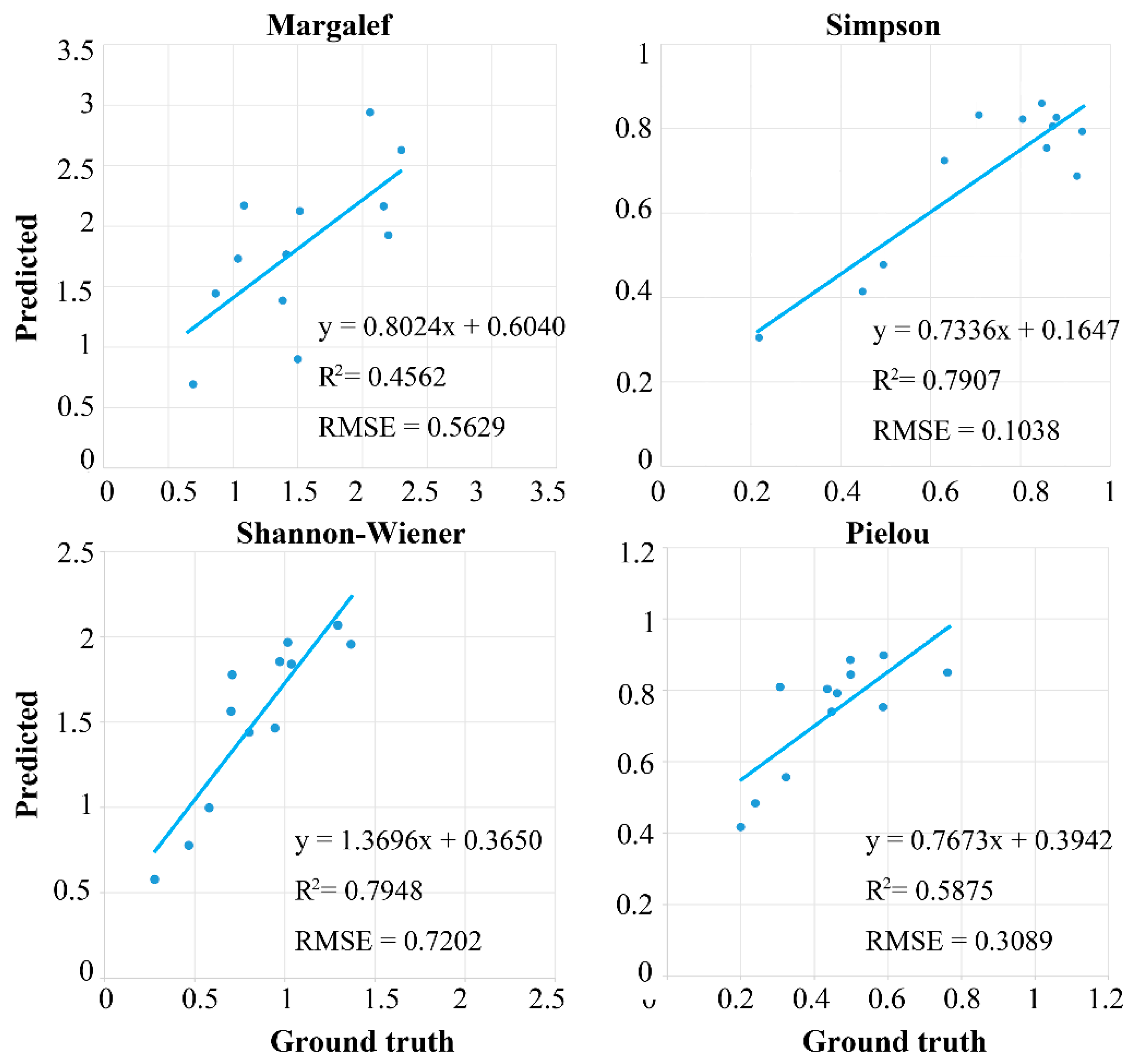
4.2.2. Accuracy Assessment

The diversity indices at the 12 field-surveyed plots were calculated according to the detected tree numbers and predicted tree species in each plot. The ground truth species richness and diversity in the very plot were both calculated with the actual number of tree species.

Table 4. The field-surveyed and predicted tree species richness.

Species Richness	Plot Number
	1	2	3	4	5	6	7	8	9	10	11	12
Ground truth	8	9	4	6	7	3	5	5	4	6	8	5
Prediction	9	8	6	4	7	3	5	9	6	8	11	6

Note: Ground truth means the actual number of tree species in the field survey, and prediction denotes the predicted number of tree species by our solution.

shows the predicted species richness compared to the ground truth. The predicted species richness was sometimes higher than the field-surveyed values (RMSE = 1.91). Figure 6 shows the validation of the four species indices calculated by VGG16 prediction. The results of the Simpson index (R² = 0.7907, RMSE = 0.1038) and the Shannon–Wiener index (R² = 0.7948, RMSE = 0.7202) were much better than those of Margalef (R² = 0.4562, RMSE = 0.5629) and Pielou (R² = 0.5875, RMSE = 0.3089). We also mapped the diversity at two other scales (i.e., 10 and 20 m) (Figure 7), which provided different patterns compared with the 30 m scale. The diversity was reduced in the two smaller scales, and the accuracy decreased at smaller spatial scales.

5. Discussion

Compared with pixel-based classification methods for tree species, our study at the individual tree level made better use of spatial context information. The convolutional layers involve the neighbors of a pixel, which can provide the texture information and spatial relationships of ground objects, while only the spectral features are employed in the pixel-based method. Although only RGB images were used for classification, the deep CNNs could generalize well to samples over different image perspectives or light conditions (Figure 8), and good accuracies were obtained. Among the three deep learning methods, networks with a deeper architecture (VGG16 and ResNet50) achieved better accuracies than AlexNet, indicating that richer features can be extracted by different levels of CNN layers. In the literature, ResNet50 has been shown to perform well [41], as its residual learning is based on the identity and projection shortcuts. However, VGG16 performed slightly better than it in this study, which might have been due to our specific individual tree datasets. Each tree species was similar in terms of the RGB images, so the deeper network of ResNet50 might have been overfitted in the training phase, which led to slightly poorer results than those from studies in other applications [50]. Both VGG16 and ResNet50 are well-suited for patch-based tree species classification, and there were only small performance differences. Moreover, the class merging strategy we used also influenced the model performance. The class of “Others” could contain a number of different tree species with various colors or textures. Although VGG16 could identify different tree species according to the high-level features extracted, the softmax classifier could not assign an appropriate label for the class of “Others”. Finally, it could assign a label from 0 to 17 (the dominant tree species which had similar features to the predicted one), leading to overestimation.

The method that we employed to isolate individual trees may have influenced the results of the biodiversity mapping. The algorithm was designed for mixed pines and deciduous trees [37], and the accuracy in this study was about 84.20% in terms of correlation coefficient R. It might not have worked well in some forest types in our study area. The individual tree detection method could be further refined by using species-specific models. Moreover, the algorithm is based on canopy height and, thus, only the trees in the upper canopy can be identified. It is meaningful to derive the whole structure feature of a tree, such as appending the stem information, from the LiDAR point clouds. Although challenges exist in individual tree isolation and tree species classification, the results of biodiversity mapping were satisfactory in a way. The Simpson index and the Shannon–Wiener index achieved high accuracy, with R² = 0.79.

The success of transferring our solution to other regions is promising. First, the development of UAV technology makes forest image data acquirement easier. UAV LiDAR and optical sensors can obtain higher-spatial-resolution LiDAR point clouds and images, and even higher-spectral-resolution images. Second, the performance of deep-learning-based approaches depends on the training data, that is, the tree species training sample and its quality. As long as the tree sample can be measured well in field work, deep learning networks will work well. Further, it is beneficial to collect tree samples with the aid of crowd sourcing. In terms of the sampled area in species diversity, our method is also applicable for other scales (50 × 50 m, 90 × 90 m, etc.), depending on the quadrat size in the field work or the requirements of species diversity estimation.

6. Conclusions

The results of this study indicate the potential of deep learning methods for applications in tree species diversity mapping with high-resolution RGB images and LiDAR data. Our proposed three-step workflow achieved accuracies of R²_{Shannon–Wiener} = 0.7948, RMSE_{Shannon–Wiener} = 0.7202; R²_Simpson = 0.7907, RMSE_Simpson = 0.1038; R²_Margalef = 0.4562, RMSE_Margalef = 0.5629; and R²_Pielou = 0.5875, RMSE_Pielou = 0.3053. The method design as well as the deep learning technology also allow the processing of large datasets and have the potential for transfer to other forest regions due to on-the-fly data acquisition and the processing capability.

A comparison of three deep learning algorithms showed that deep CNN architectures can perform well in tree species diversity mapping. VGG16 achieved a slightly better performance than ResNet50 due to the characteristics of the tree samples. The results of only using RGB images in our study show the potential of tree species diversity mapping. It can be expected to be able to predict diversity more accurately with the improved estimation of individual tree isolation and the addition of other bands (such as near-infrared and red-edge bands) in tree species classification. We conclude that our proposed solution using deep learning approaches is suited to map tree species diversity in the Haizhu Wetland.

References

1. Schäfer, E.; Heiskanen, J.; Heikinheimo, V.; Pellikka, P. Mapping tree species diversity of a tropical montane forest by unsupervised clustering of airborne imaging spectroscopy data. Ecol. Indic. 2016, 64, 49–58. [Google Scholar] [CrossRef]
2. Ferreira, M.P.; Zortea, M.; Zanotta, D.C.; Shimabukuro, Y.E.; de Souza Filho, C.R. Mapping tree species in tropical seasonal semi-deciduous forests with hyperspectral and multispectral data. Remote Sens. Environ. 2016, 179, 66–78. [Google Scholar] [CrossRef]
3. Magurran, A.E. Ecological Diversity and Its Measurement; Princeton University Press: Princeton, NJ, USA, 1988. [Google Scholar]
4. Gillson, L.; Duffin, K. Thresholds of potential concern as benchmarks in the management of African savannahs. Philos. Trans. R. Soc. B Biol. Sci. 2007, 362, 309–319. [Google Scholar] [CrossRef]
5. Madonsela, S.; Cho, M.A.; Ramoelo, A.; Mutanga, O.; Naidoo, L. Estimating tree species diversity in the savannah using NDVI and woody canopy cover. Int. J. Appl. Earth Obs. Geoinf. 2018, 66, 106–115. [Google Scholar] [CrossRef]
6. Jetz, W.; Cavender-Bares, J.; Pavlick, R.; Schimel, D.; Davis, F.W.; Asner, G.P.; Guralnick, R.; Kattge, J.; Latimer, A.M.; Moorcroft, P. Monitoring plant functional diversity from space. Nat. Plants 2016, 2, 16024. [Google Scholar] [CrossRef] [PubMed]
7. Nagendra, H.; Lucas, R.; Honrado, J.P.; Jongman, R.H.; Tarantino, C.; Adamo, M.; Mairota, P. Remote sensing for conservation monitoring: Assessing protected areas, habitat extent, habitat condition, species diversity, and threats. Ecol. Indic. 2013, 33, 45–59. [Google Scholar] [CrossRef]
8. Lopatin, J.; Dolos, K.; Hernández, H.; Galleguillos, M.; Fassnacht, F. Comparing generalized linear models and random forest to model vascular plant species richness using LiDAR data in a natural forest in central Chile. Remote Sens. Environ. 2016, 173, 200–210. [Google Scholar] [CrossRef]
9. Nagendra, H.; Gadgil, M. Satellite imagery as a tool for monitoring species diversity: An assessment. J. Appl. Ecol. 1999, 36, 388–397. [Google Scholar] [CrossRef]
10. Nagendra, H. Using remote sensing to assess biodiversity. Int. J. Remote Sens. 2001, 22, 2377–2400. [Google Scholar] [CrossRef]
11. Kuenzer, C.; Ottinger, M.; Wegmann, M.; Guo, H.; Wang, C.; Zhang, J.; Dech, S.; Wikelski, M. Earth observation satellite sensors for biodiversity monitoring: Potentials and bottlenecks. Int. J. Remote Sens. 2014, 35, 6599–6647. [Google Scholar] [CrossRef]
12. Zhao, Y.; Zeng, Y.; Zheng, Z.; Dong, W.; Zhao, D.; Wu, B.; Zhao, Q. Forest species diversity mapping using airborne LiDAR and hyperspectral data in a subtropical forest in China. Remote Sens. Environ. 2018, 213, 104–114. [Google Scholar] [CrossRef]
13. Yang, C.; Everitt, J.H.; Fletcher, R.S.; Jensen, R.R.; Mausel, P.W. Evaluating AISA+ hyperspectral imagery for mapping black mangrove along the South Texas Gulf Coast. Photogramm. Eng. Remote Sens. 2009, 75, 425–435. [Google Scholar] [CrossRef]
14. Nevalainen, O.; Honkavaara, E.; Tuominen, S.; Viljanen, N.; Hakala, T.; Yu, X.; Hyyppä, J.; Saari, H.; Pölönen, I.; Imai, N. Individual tree detection and classification with UAV-based photogrammetric point clouds and hyperspectral imaging. Remote Sens. 2017, 9, 185. [Google Scholar] [CrossRef]
15. Dalponte, M.; Bruzzone, L.; Gianelle, D. Tree species classification in the Southern Alps based on the fusion of very high geometrical resolution multispectral/hyperspectral images and LiDAR data. Remote Sens. Environ. 2012, 123, 258–270. [Google Scholar] [CrossRef]
16. Goodenough, D.G.; Dyk, A.; Niemann, K.O.; Pearlman, J.S.; Chen, H.; Han, T.; Murdoch, M.; West, C. Processing Hyperion and ALI for forest classification. IEEE Trans. Geosci. Remote Sens. 2003, 41, 1321–1331. [Google Scholar] [CrossRef]
17. Féret, J.-B.; Asner, G.P. Semi-supervised methods to identify individual crowns of lowland tropical canopy species using imaging spectroscopy and LiDAR. Remote Sens. 2012, 4, 2457–2476. [Google Scholar] [CrossRef]
18. Hakkenberg, C.; Zhu, K.; Peet, R.; Song, C. Mapping multi-scale vascular plant richness in a forest landscape with integrated Li DAR and hyperspectral remote-sensing. Ecology 2018, 99, 474–487. [Google Scholar] [CrossRef]
19. Getzin, S.; Wiegand, K.; Schöning, I. Assessing biodiversity in forests using very high-resolution images and unmanned aerial vehicles. Methods Ecol. Evolut. 2012, 3, 397–404. [Google Scholar] [CrossRef]
20. Carleer, A.; Wolff, E. Exploitation of very high resolution satellite data for tree species identification. Photogramm. Eng. Remote Sens. 2004, 70, 135–140. [Google Scholar] [CrossRef]
21. van Lier, O.R.; Fournier, R.A.; Bradley, R.L.; Thiffault, N. A multi-resolution satellite imagery approach for large area mapping of ericaceous shrubs in Northern Quebec, Canada. Int. J. Appl. Earth Obs. Geoinform. 2009, 11, 334–343. [Google Scholar] [CrossRef]
22. Wang, L.; Sousa, W.P.; Gong, P.; Biging, G.S. Comparison of IKONOS and QuickBird images for mapping mangrove species on the Caribbean coast of Panama. Remote Sens. Environ. 2004, 91, 432–440. [Google Scholar] [CrossRef]
23. Sasaki, T.; Imanishi, J.; Ioki, K.; Morimoto, Y.; Kitada, K. Object-based classification of land cover and tree species by integrating airborne LiDAR and high spatial resolution imagery data. Lands. Ecol. Eng. 2012, 8, 157–171. [Google Scholar] [CrossRef]
24. Clark, M.L.; Roberts, D.A.; Clark, D.B. Hyperspectral discrimination of tropical rain forest tree species at leaf to crown scales. Remote Sens. Environ. 2005, 96, 375–398. [Google Scholar] [CrossRef]
25. Rosenfeld, A.; Zemel, R.; Tsotsos, J.K. The elephant in the room. arXiv 2018, arXiv:1808.03305. [Google Scholar]
26. Ma, L.; Liu, Y.; Zhang, X.; Ye, Y.; Yin, G.; Johnson, B.A. Deep learning in remote sensing applications: A meta-analysis and review. ISPRS J. Photogramm. Remote Sens. 2019, 152, 166–177. [Google Scholar] [CrossRef]
27. Sun, Y.; Zhang, X.; Xin, Q.; Huang, J. Developing a multi-filter convolutional neural network for semantic segmentation using high-resolution aerial imagery and LiDAR data. ISPRS J. Photogramm. Remote Sens. 2018, 143, 3–14. [Google Scholar] [CrossRef]
28. Xu, G.; Zhu, X.; Fu, D.; Dong, J.; Xiao, X. Automatic land cover classification of geo-tagged field photos by deep learning. Environ. Model. Softw. 2017, 91, 127–134. [Google Scholar] [CrossRef]
29. Sun, Z.; Zhao, X.; Wu, M.; Wang, C. Extracting Urban Impervious Surface from WorldView-2 and Airborne LiDAR Data Using 3D Convolutional Neural Networks. J. Indian Soc. Remote Sens. 2019, 47, 401–412. [Google Scholar] [CrossRef]
30. Huang, J.; Zhang, X.; Xin, Q.; Sun, Y.; Zhang, P. Automatic building extraction from high-resolution aerial images and LiDAR data using gated residual refinement network. ISPRS J. Photogramm. Remote Sens. 2019, 151, 91–105. [Google Scholar] [CrossRef]
31. Chen, Z.; Chen, Z. Rbnet: A deep neural network for unified road and road boundary detection. Int. Conf. Neural Inf. Process. 2017, 677–687. [Google Scholar] [CrossRef]
32. Du, Z.; Yang, J.; Ou, C.; Zhang, T. Smallholder Crop Area Mapped with a Semantic Segmentation Deep Learning Method. Remote Sens. 2019, 11, 888. [Google Scholar] [CrossRef]
33. Persello, C.; Tolpekin, V.; Bergado, J.; de By, R. Delineation of agricultural fields in smallholder farms from satellite images using fully convolutional networks and combinatorial grouping. Remote Sens. Environ. 2019, 231, 111253. [Google Scholar] [CrossRef] [PubMed]
34. Sylvain, J.-D.; Drolet, G.; Brown, N. Mapping dead forest cover using a deep convolutional neural network and digital aerial photography. ISPRS J. Photogramm. Remote Sens. 2019, 156, 14–26. [Google Scholar] [CrossRef]
35. Flood, N.; Watson, F.; Collett, L. Using a U-net convolutional neural network to map woody vegetation extent from high resolution satellite imagery across Queensland, Australia. Int. J. Appl. Earth Obs. Geoinform. 2019, 82, 101897. [Google Scholar] [CrossRef]
36. Li, W.; Fu, H.; Yu, L.; Cracknell, A. Deep learning based oil palm tree detection and counting for high-resolution remote sensing images. Remote Sens. 2016, 9, 22. [Google Scholar] [CrossRef] [Green Version]
37. Popescu, S.C.; Wynne, R.H.; Nelson, R.F. Estimating plot-level tree heights with lidar: Local filtering with a canopy-height based variable window size. Comput. Electron. Agric. 2002, 37, 71–95. [Google Scholar] [CrossRef]
38. Krizhevsky, A.; Sutskever, I.; Hinton, G.E. Imagenet classification with deep convolutional neural networks. Adv. Neural Inf. Process. Syst. 2012, 25, 1097–1105. [Google Scholar] [CrossRef]
39. Simonyan, K.; Zisserman, A. Very deep convolutional networks for large-scale image recognition. arXiv 2014, arXiv:1409.1556. Available online: https://arxiv.org/abs/1409.1556 (accessed on 10 April 2015).
40. Szegedy, C.; Liu, W.; Jia, Y.; Sermanet, P.; Reed, S.; Anguelov, D.; Erhan, D.; Vanhoucke, V.; Rabinovich, A. Going deeper with convolutions. In Proceedings of the IEEE Conference on Computer Vision and Pattern Recognition, Boston, MA, USA, 7–12 June 2015; pp. 1–9. [Google Scholar]
41. He, K.; Zhang, X.; Ren, S.; Sun, J. Deep residual learning for image recognition. In Proceedings of the IEEE Conference on Computer Vision and Pattern Recognition, Las Vegas, NV, USA, 27–30 June 2016; pp. 770–778. [Google Scholar]
42. Rocchini, D.; Hernández-Stefanoni, J.L.; He, K.S. Advancing species diversity estimate by remotely sensed proxies: A conceptual review. Ecol. Inf. 2015, 25, 22–28. [Google Scholar] [CrossRef]
43. Margalef, D. Information theory in ecology, General systems. Transl. Mem. Real Acad. Cienc. Artes Barcelona 1958, 32, 373–449. [Google Scholar]
44. Simpson, E.H. Measurement of diversity. Nature 1949, 163, 688. [Google Scholar] [CrossRef]
45. Shannon, C.; Weiner, W. The Mathematical Theory of Communication; Urban University Illinois Press: Champaign, IL, USA, 1963; 125p. [Google Scholar]
46. Pielou, E.C. Species-diversity and pattern-diversity in the study of ecological succession. J. Theor. Biol. 1966, 10, 370–383. [Google Scholar] [CrossRef]
47. Jia, Y.; Shelhamer, E.; Donahue, J.; Karayev, S.; Long, J.; Girshick, R.B.; Guadarrama, S.; Darrell, T. Caffe: Convolutional Architecture for Fast Feature Embedding. ACM Multimed. 2014, 675–678. [Google Scholar] [CrossRef]
48. Kingma, D.P.; Ba, J. Adam: A Method for Stochastic Optimization. In Proceedings of the International Conference on Learning Representations, San Diego, CA, USA, 7–9 May 2015. [Google Scholar]
49. Martin, D.R.; Fowlkes, C.C.; Malik, J. Learning to detect natural image boundaries using local brightness, color, and texture cues. IEEE Trans. Pattern Anal. Mach. Intell. 2004, 26, 530–549. [Google Scholar] [CrossRef]
50. Jung, H.; Choi, M.-K.; Jung, J.; Lee, J.-H.; Kwon, S.; Young Jung, W. ResNet-based vehicle classification and localization in traffic surveillance systems. In Proceedings of the IEEE Conference on Computer Vision and Pattern Recognition Workshops, Honolulu, HI, USA, 21–26 July 2017; pp. 61–67. [Google Scholar]
Figure 1. The location of Haizhu Wetland and three separate parts with true-color composites in the Haizhu Wetland were selected as the study area. Area A is also referred to as Haizhu Lake Park, and a forest (dominant by broadleaved trees) grows along the lake. Area B is a semiconstructed wetland mixed with various broadleaved trees, including flowering and fruit trees. Area C is mainly covered by neatly arranged fruit trees. The red squares in Areas A and B denote the locations of the field-surveyed plots.
Forests 10 01047 g001
Figure 2. The flowchart that includes three main steps for identification of tree species based on the deep learning approaches.
Forests 10 01047 g002
Figure 3. The RGB image was cropped into patches (red squares) based on the detected tree locations (red stars) with a patch size of 64 × 64 pixels each.
Forests 10 01047 g003
Figure 4. The architectures of the three deep convolutional neural networks used in our tree species classification. Adapted from Krizhevsky et al. [38], Simonyan and Zisserman [39], and He et al. [41]. The numbers on the top of each box are the number of bands of the feature maps, while the numbers on the bottom are the size (height and width) of the feature map.
Forests 10 01047 g004
Figure 5. Tree species diversity mapping with a spatial resolution of 30 m in the three parts of Haizhu Wetland.
Forests 10 01047 g005
Figure 6. Field survey diversity index compared with the VGG16 predicted value.
Forests 10 01047 g006
Figure 7. Tree species diversity maps at the spatial resolutions of 10 and 20 m. M_10m and M_20m represent the Margalef index at 10 and 20 m scales, respectively. SW_10m and SW_20m are for the Shannon–Wiener index at 10 and 20 m scales, respectively.
Forests 10 01047 g007
Figure 8. Tree patch samples over different image perspectives or light conditions. The first row is samples of banyan tree, while the second row is sakura tree.
Forests 10 01047 g008