The Cumulative Effects of Forest Disturbance and Climate Variability on Streamflow in the Deadman River Watershed


1
Department of Earth, Environmental and Geographic Sciences, University of British Columbia Okanagan, 1177 Research Road, Kelowna, BC V1V 1V7, Canada
2
Department of Civil Engineering, University of Victoria, 3800 Finnerty Road, Victoria, BC V8P 5C2, Canada
*
Author to whom correspondence should be addressed.
Forests 2019, 10(2), 196; https://0-doi-org.brum.beds.ac.uk/10.3390/f10020196
Submission received: 11 January 2019
/
Revised: 13 February 2019
/
Accepted: 20 February 2019
/
Published: 22 February 2019
(This article belongs to the Special Issue Forest Hydrology and Watershed)
Abstract
:Climatic variability and cumulative forest cover change are the two dominant factors affecting hydrological variability in forested watersheds. Separating the relative effects of each factor on streamflow is gaining increasing attention. This study adds to the body of literature by quantifying the relative contributions of those two drivers to the changes in annual mean flow, low flow, and high flow in a large forested snow dominated watershed, the Deadman River watershed (878 km2) in the Southern Interior of British Columbia, Canada. Over the study period of 1962 to 2012, the cumulative effects of forest disturbance significantly affected the annual mean streamflow. The effects became statistically significant in 1989 at the cumulative forest disturbance level of 12.4% of the watershed area. The modified double mass curve and sensitivity-based methods consistently revealed that forest disturbance and climate variability both increased annual mean streamflow during the disturbance period (1989–2012), with an average increment of 14 mm and 6 mm, respectively. The paired-year approach was used to further investigate the relative contributions to low and high flows. Our analysis showed that low and high flow increased significantly by 19% and 58%, respectively over the disturbance period (p < 0.05). We conclude that forest disturbance and climate variability have significantly increased annual mean flow, low flow and high flow over the last 50 years in a cumulative and additive manner in the Deadman River watershed.
1. Introduction
Forested watersheds are important sources of streamflow, water regulation and generation for more than 30% of the world’s population [1,2]. Changes in forest cover have important effects on the sustainability of water resources, aquatic habitat, and many other ecological functions. In forested watersheds, forest cover change and climate variability are regarded as the two main drivers of hydrological variation [3,4]. The compounding effects of climate variability and land cover change (e.g., forest harvesting, land use conversion) have driven scientific research to focus on how these drivers and their interactions affect the hydrological regime [5,6,7,8,9].
The effect of forest cover change on streamflow has been studied for many decades, with periodic summaries consolidating key findings [4,9,10,11]. However, most research has been carried out using paired watershed experiments (PWE) in small watersheds (<100 km2) since the 1910s with long term land cover and streamflow data. The inability to simply extrapolate results from the PWE to watersheds of different sizes, topography, climate and land cover types, suggests an important need to study hydrological responses to forest changes at other spatial scales. This gap is recently and clearly recognized in a recent global assessment report on forests and water [12]. Additionally, advances have been made in hydrological modeling (e.g., the Soil and Water Assessment Tool) and statistical methods such as time-trend analysis, sensitivity-based method, double mass curves (DMC), and those based on the Budyko theory [3,13]. These advances make it possible to evaluate the forest-water relationship in large watersheds.
Numerous forest indicators have been used to characterise forest change through time in hydrological studies including: percentage forested [14], the area disturbed, and remotely sensed vegetation indices such as the Normalized Difference Vegetation Index (NDVI) [2,15], Leaf Area Index (LAI) [16,17,18], and normalized burn ratio (NBR) [19]. Although these indices have been widely implemented in assessing spatial and temporal dynamics of forest cover, they do not explicitly account for hydrological recovery due to regeneration following forest disturbance, and consequently cumulative effects on hydrology. Cumulative effects are defined as the combined results from actions that are individually minor but collectively significant in the past, present, and foreseeable future [20,21]. Therefore, a comprehensive index is required, which can account for spatial and temporal cumulative forest cover change. ECA (equivalent clear-cut area) is calculated as the cumulative area that is clear-cut with a reduction factor implemented over time to account for hydrological recovery as the forest regenerates [22]. ECA has been widely used in scientific research and operational practices in the Pacific Northwest for decades [23,24,25,26,27], and can therefore, be a good indicator to quantify cumulative forest cover change in a watershed.
Previous studies generally conclude that deforestation increases annual mean flow (Qmean),while reforestation decreases it across multiple spatial scales [4,11], with less consistent results in the literature on low and high flows. For instance, it has been found that forest logging could increase the frequency and magnitude of high flows but is unlikely to affect large flooding events [23,28]. In snow dominated watersheds, the effect is less significant and forest disturbance has been found to advance the timing of snow-melt generated high flows [29]. The effect on low flow is tightly coupled to soil disturbance, the history of land use, and climatic regime [30,31]. Numerous studies have found that disturbance can increase low flow, however some show inconsistent results with negative and insignificant changes in low flows [26,31]. Our collective understanding of how forest cover change might affect streamflow has progressed, however, there is an increasing demand for more case studies, shown by the limited number of studies and lack of consistency or explanation of differences between results from various regions characterised with different climate regimes, forest structure, soil property, and topography [9].
The Deadman River watershed (878 km2) is located in the Southern Interior of British Columbia, Canada. It is characterised by a snow dominated hydrological regime and has experienced dramatic forest disturbance from the mountain pine beetle (MPB) infestation and forest harvesting. The significant level of forest disturbance in the watershed has raised serious concerns over alteration of the hydrological regime. To address these hydrological concerns, this study answers two research questions: 1) how have forest disturbance and climate cumulatively affected annual streamflow in Deadman River watershed, and 2) how have forest disturbance and climate cumulatively affected high and low flows?
2. Materials and Methods
2.1. Watershed Description
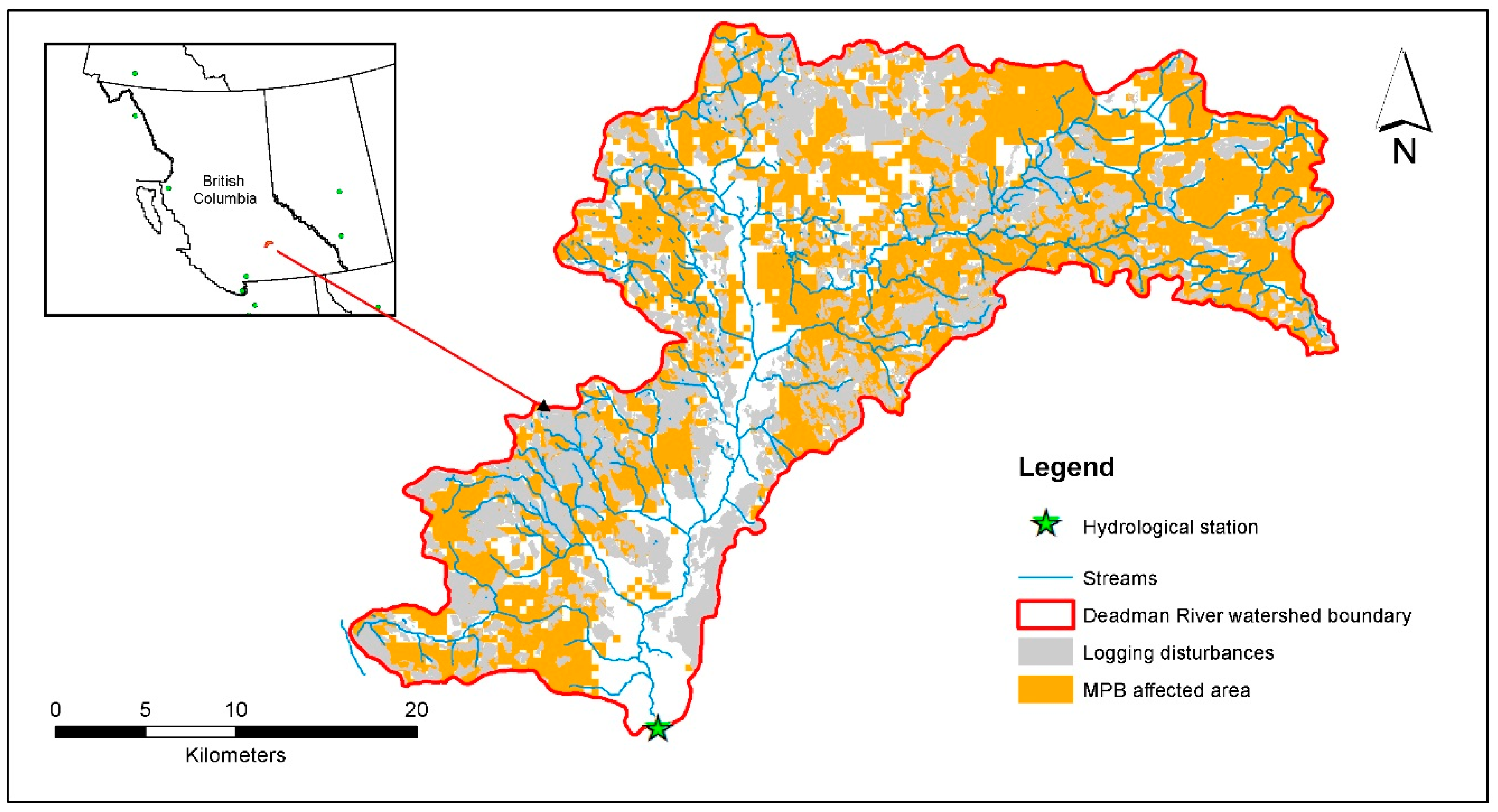
The Deadman River watershed is located in the Southern Interior of British Columbia, Canada. (Figure 1). The drainage area is 878 km2 of which 91.3% is forested, with most of the remaining area being grassland in the valley bottoms. Deadman River is an important Salmonoid-bearing river that is a tributary of Thompson River. Communities and First Nations rely directly on the water to drink, irrigate, and sustain a healthy fish population, ecological functioning and aquatic resources. The elevation ranges from 527 m above sea level at the southern outlet and main branch of the Deadman River up to 1779 m in the upper reaches to the east and west of the watershed (Figure 1). From 1962–2012, the mean daily temperature in the winter (December–February) was −6 °C and 12.9 °C in the summer (June–August). Approximately 27% of the annual precipitation (P) accumulates as snow in the winter, with the snow-melt event producing the spring freshet (Figure S1 in the Supplementary Materials (SM)). Lower elevation slopes support Douglas-fir (Pseudotsuga menziesii (Mirb.) Franco) and Lodgepole pine (Pinus contorta Douglas ex Loudon) dominated forests with smaller amounts of Spruce (Picea glauca (Moench) Voss) and Balsam (Abies lasiocarpa (Hook.) Nutt.). A small amount of agriculture and urban development dominate the valley bottom (around 1% of the total watershed area), the total area of which has not changed over the course of this study; while forestry is the main land use across the watershed [32]. The recent Province-wide mountain pine beetle (MPB) epidemic [33] has brought widespread Lodgepole pine mortality and salvage harvesting throughout the watershed (Figure 1).
2.2. Watershed Data
The age, height, density, and species composition of the forest was sourced from the 2013 provincial vegetation resources inventory (VRI). Disturbance indicators were calculated using three complementary spatial databases that are maintained by the BC Ministry of Forests, Lands and Natural Resource Operations (FLNRO). The spatial and temporal location of historical harvesting was accounted for using the FLNRO consolidated cutblocks layer (2013), wildfires from the BC wildfire database, and mountain pine beetle (MPB) disturbance from the British Columbia Mountain Pine Beetle (BCMPB) projections version 11 [33].
Daily discharge data (m3s−1) from 1960 to 2012 was acquired from Environment Canada (Station ID: 08LF027), which was standardized to millimeters (mm year−1) using watershed area (Figure S2). The watershed monthly P, mean, maximum, and minimum temperatures (Tmean, Tmax, Tmin) were derived from the ClimateBC model at the spatial resolution of 500 × 500 m [34] (Figures S3 and S4 in the SM). Elevation (m) for each VRI polygon was calculated from the FLNRO digital elevation model at a spatial resolution of 30 meters.
2.3. Cumulative Equivalent Clear-Cut Area
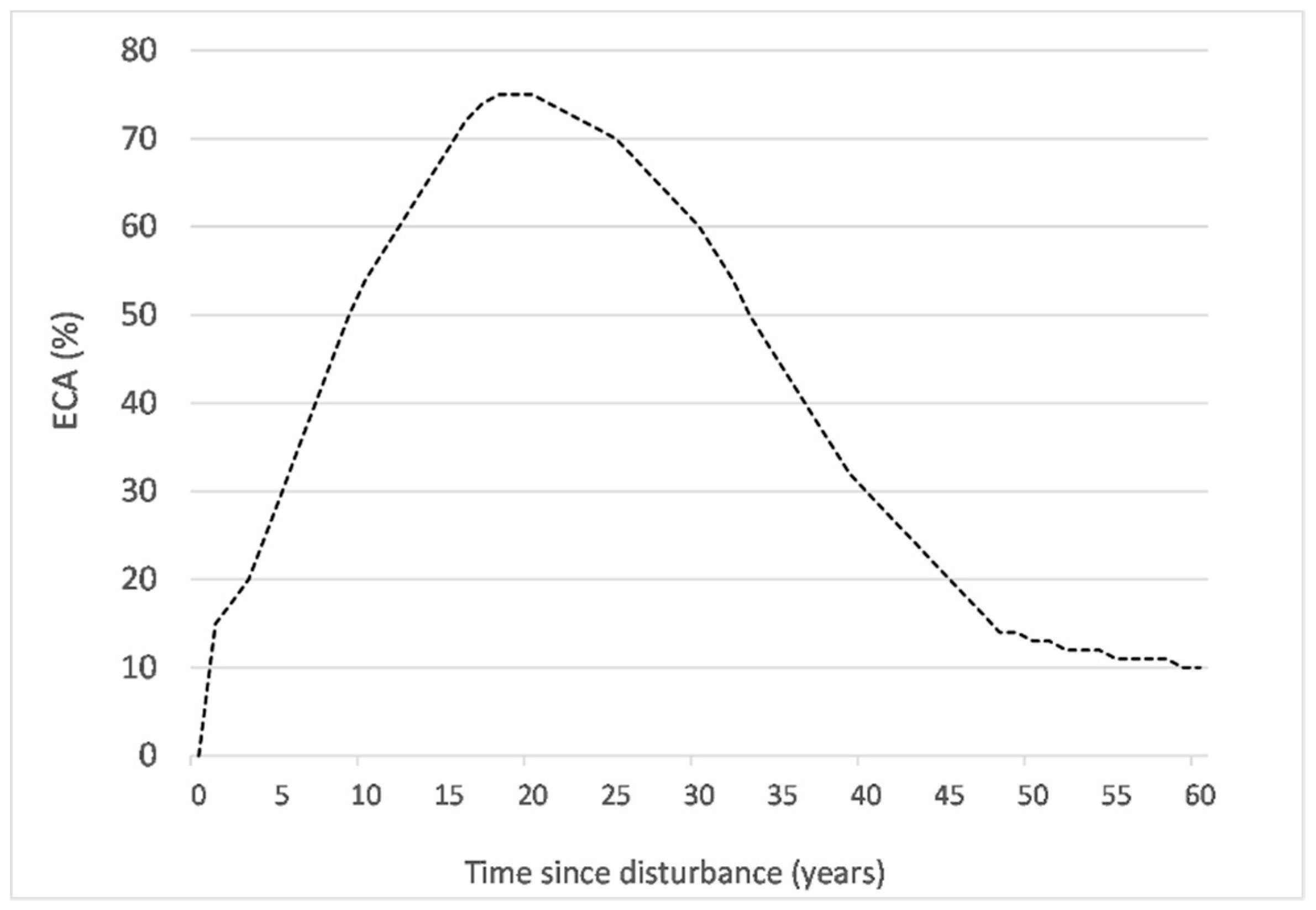
Forest logging, MPB infestation, and wildfire are the three major disturbance types and cumulate over space and time in the study watershed (Figure 1). Cumulative equivalent clear-cut area (CECA) was used to account for cumulative forest disturbance at the watershed level [22,35]. At the stand level, equivalent clear-cut area (ECA) is defined as the area that has been clear-cut, killed by fire, or infested by MPB, with a reduction factor to account for hydrological recovery as the forest regenerates. All forest logging in the area is clear-cut. Following the watershed assessment procedure in British Columbia [27], the ECA is set at 100% after harvesting, reflecting changes in hydrological processes such as infiltration, evapotranspiration, and run-off. Stand height was used to represent the relationship between forest growth and hydrological recovery [22,27] (Table 1). Hydrological recovery after wildfire was assumed to follow the same relationship as harvesting [36]. The hydrological recovery of a forest stand is related to its growth rate over time and is therefore determined by many factors including disturbance type, climate, and tree species. Accounting for this, stand height is projected through time using standard models that are calibrated in British Columbia. The Variable Density Yield Prediction model version 7 (VDYP7) is used for stands of natural origin (wildfire) and the Table Interpolation Program for Stand Yields model version 4.3 (TIPSYv4.3) is used for stands that regenerate after harvesting. In MPB affected forest, the ECA shown in Figure 2 [29,37] is applied to the affected portion of a stand. It follows an asymmetrical bell-shaped curve through time as tree death and needle drop occur gradually over years [38,39] and regeneration and hydrological recovery starts around 20 years. Stand-level ECA values are summed annually to give the watershed–level CECA timeseries.
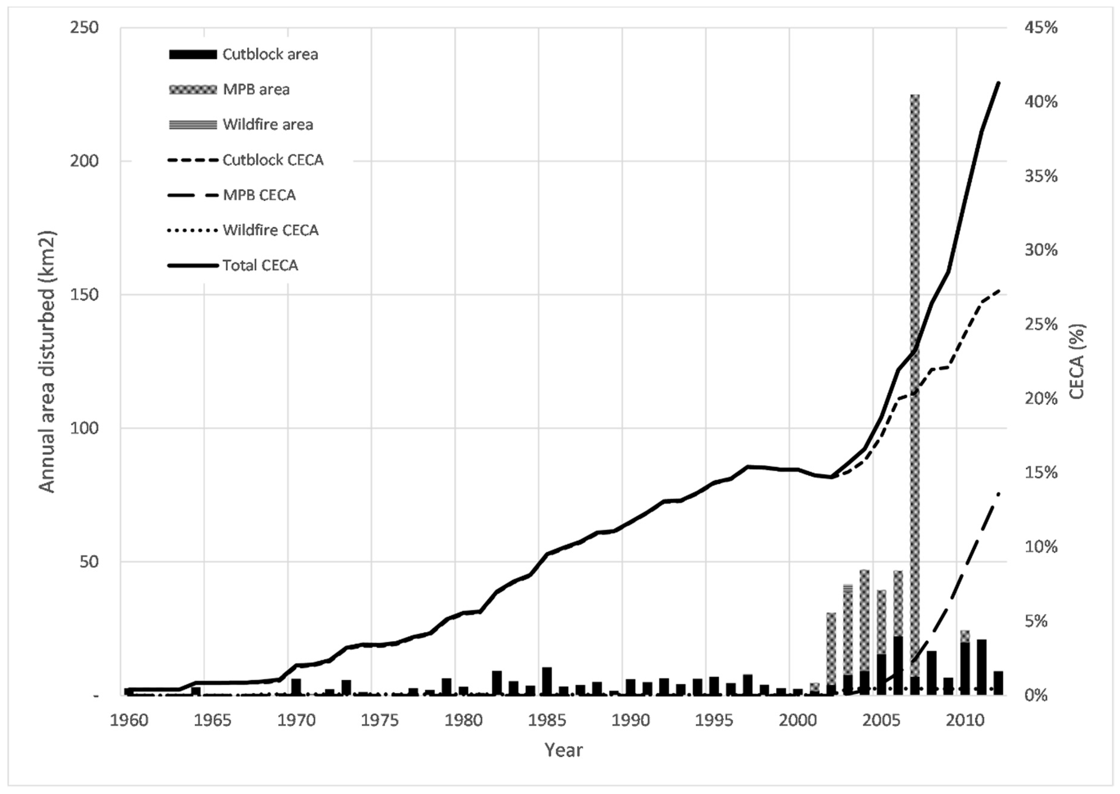
In 2012, the CECA was 41.3% of the watershed area (Figure 3). Logging was the dominant disturbance type through the study period. The average annual harvest rate in the Deadman River watershed was 4 km2 year−1 from 1960 till 1999. From the year 2000 onwards, this rate increased to an average of 11 km2 year−1. In 2012, the CECA from logging was 27.2% of the watershed area. MPB affected a total of 370 km2 since 2000, a rate of 46 km2 year−1 (Figure 3). The CECA of MPB in 2012 was 13.6%. Wildfire is an insignificant disturbance agent during the study period with only 3 km2 in total. The total CECA rose from 0% in 1960 to 41% in 2012. Overall, the Deadman River watershed has experienced significant forest disturbance.
2.4. Cross-Correlation Analysis
Cross-correlation analysis is an effective method to examine whether there are significant relationships between two time series variables. The advantage of cross-correlation is that it can remove autocorrelations existing in data series and identify lagged causality between them [29]. In this study, cross-correlation tests were used to detect relationships and lagged effects between cumulative forest change (CECA) and three flow variables, including: annual mean streamflow (Qmean), a low flow parameter (Q95%) which is defined as the daily flow equalled or exceeded for 95% of days in a year, and high flow parameter (Q5%) which is the daily flow equalled or exceeded 5% of days in year.
All variables were pre-whitened to remove autocorrelation by fitting Autoregressive Integrated Moving Average (ARIMA) models in R software [40]. The ndiffs function from the forecast package [41] was first used to find the level of differencing needed to achieve stationarity and then the ARIMA model with the best performancewas selected for cross-correlation analysis [42]. Cross-correlation analysis of ARIMA model residuals was carried out in R using the ccf function from the forecast package [41]. The correlation coefficient and significant lags are used to assess if there is a correlation between tested variables.
2.5. Quantifying the Effects of Forest Disturbance and Climate Variability on Streamflow Components
Three complementary statistical methods were used to make a robust assessment of the separate effects of forest disturbance and climate variation on streamflow components. The modified double mass curve (MDMC) method and sensitivity-based method were applied to Qmean, while the paired-year approach can be used for Qmean, Q5% and Q95%.
2.5.1. Timeseries Trend Analysis
As a first step, the Mann–Kendall test [43,44] was used to assess what trends exist in the climatic and hydrological data over the study period, helping with the interpretation of results. The Mann–Kendall non-parametric test is widely used in hydrology for the trend detection [23]. Prior to implementing the Mann–Kendall test, each timeseries was pre-whitened to remove the influence of serial correlations [45], following the process recommended in Yue et al. [46]. However, Razavi and Vogel [47] recently demonstrated how pre-whitening can underestimate extreme conditions in hydrological timeseries analysis, leading to a potentially conservative correlation in this analysis. All statistical tests are at a significance level of 5%.
2.5.2. Modified Double Mass Curve
A modified double mass curve (MDMC) is a graph of cumulative annual Qmean versus cumulative effective precipitation (Pe) which is the difference between annual P and actual evapotranspiration (AET) [3,22]. Annual potential evapotranspiration (PET) was estimated as the average of the Priestley–Taylor [48] and Hamon method [49,50,51] and then AET was calculated as the average of the Budyko [52] and Zhang’s [53] equations. The basic assumptions of the MDMC are 1) the linear relationship holds between the Pe and Qmean; and 2) all climate variability is lumped into P and ET [22,54]. In a period with no forest disturbance (reference period), the slope of the MDMC should be straight, and a break point in this line suggests a regime shift in annual mean flow caused by forest disturbance (disturbance period) [3]. The Pettitt break point test was introduced to detect the statistically significant break point between the reference and disturbance periods [55]. Before carrying out the Pettitt test, autocorrelations in the MDMC slope were removed following the methodology found in Yue et al. [46]. To validate the statistical significance of the break point, the nonparametric Mann–Whitney U test Z statistic was adopted [8,30,56]. The linear relationship in the reference period was used to predict the cumulative annual streamflow for the disturbance period, with the difference between this and the observed line regarded as the cumulative impact of forest change on streamflow (∆Qf). The deviations caused by climate variability on each annual streamflow component can be determined using Equation (1).
where, ∆Q, ∆Qf, and ∆Qc are the deviations of each annual streamflow between disturbance and reference periods, annual flow deviations caused by forest disturbance, and annual flow deviations caused by climate variability, respectively. The relative contributions of forest disturbance and climate variability to Qmean is calculated from their respective proportion of ∆Q [22].
2.5.3. Sensitivity-Based Method
The sensitivity-based approach assumes that the change in Qmean can be determined using Equation (2) [57,58].
where, ∆P, ∆PET, and ∆Qc are the difference in annual P, PET, and Q due to climate between reference and disturbance periods, respectively. β and γ are the sensitivity coefficients of streamflow to P and PET [36]. β and γ can be derived from Equations (3) and (4) below, where ω is assumed to be 2 for a predominantly forested watershed.
As a result, the effects of forest change on Qmean can be derived using Equation (1).
2.5.4. Paired-Year Approach
Similar to the approaches for assessing the cumulative effects of forest disturbance on Qmean, the effects of climate variability on Q5% and Q95% should be removed first. The paired-year approach has been effectively used to quantify the cumulative effects of forest disturbance on flow regimes across various climatic regions [35,42] and was selected for this study. The paired-year approach assumes that flow changes are mainly attributed to cumulative forest disturbance when climate conditions between the reference and disturbance year are similar. To identify climatic variables that can be used as proxies for equivalent climate conditions, the following steps are used: (1) Kendall tau correlation analyses are used to select the statistical relationship between flow (Q5% and Q95%) and seasonal or annual climate variables, respectively (Table S1). (2) Once key climate variables were determined, several combinations or sets of the selected climate variables were composed. (3) Each set of the climate variables and the set of Q5% and Q95% serve as inputs for the canonical correlation analyses [35], the approach used to examine correlations between two sets of variables. To ensure that all combinations of climate variables were tested thoroughly, we also selected climate variables that were not statistically related to the Q5% and Q95% for the canonical correlation analyses. A total of 30 sets were tested and finally the Tmean, Tmax, minimum summer temperature, winter P of the antecedent year and spring P in the current year, were determined as the controlling climate variables. To ensure a reliable pairing, a threshold of 10% biases were allowed in each climatic variable (Table S2). (4) As a result, ten pairs of years were chosen to compare Q5% and Q95% with similar climate (Table S3). The differences between each pair of years are denoted as the effects of cumulative forest disturbances on Q5% and Q95%. (5) The Mann–Whitney U test is further used to confirm whether Q5% and Q95% between the reference and disturbance are statistically significant [35]. As such, the cumulative forest disturbance on Q5% and Q95% were quantified.
3. Results
3.1. Time-Trend Analysis of the Hydrometeorological Variables
Mann–Kendall trend analysis was used to study the annual and seasonal trends in hydrometeorological variables for the Deadman River watershed across the whole study period. Table 2 presents the results of this analysis after pre-whitening following Yue et al. [46]. Although only annual temperatures experienced significant upwards trends (at a significance level (p-value) < 0.05), spring and summer Tmin were significant. Related to increasing Tmean, annual PET also exhibited a significant upward trend. Spring P was the only season that showed a significant increasing trend for P. For streamflow, only autumn Qmean and Q95% showed an increasing trend with no corresponding significant climate trend. The increasing trends in temperatures and PET may, therefore, play a role in reducing streamflow, while increased spring P may increase spring streamflow. While, time-trend analysis is useful to help understand hydrologic behaviour, it does not have explanatory power on its own. In addition, recent reviews by Razavi and Vogel [47] and Serinaldi et al. [59] have exposed shortcomings when used in hydrological timeseries analysis. Therefore, we use the results from time-trend analysis with caution and as one piece to inform the overall picture.
3.2. Cross-Correlation between Forest Disturbance and Streamflow Regime Components
Annual hydrological and CECA timeseries were first pre-whitened to remove serial correlations using ARIMA models as listed in Table 3. The pre-whitened variables from this process were used in the cross-correlation analysis. Cross-correlation analysis cannot prove causality but is used to calculate the statistical relationship between two data series considering the displacement (“lag”) of one relative to the other. Cross-correlation analysis revealed that CECA is significantly related to Qmean, Q5% and Q95% as shown by significant correlation coefficients for all hydrologic variables. The lags indicate that the response of hydrological variables are 8, 8, and 4 years after the change in CECA. The lag detected by cross-correlation reflects that the observed response of streamflow to forest cover change only occurs when disturbance accumulates to certain amount in a watershed. Additionally, changes caused by MPB mortality such as the cessation of root functioning, needle drop and decomposition occur gradually over a number of years [60]. The positive correlation coefficient implies that a higher level of cumulative disturbance, approximated by CECA, likely results in higher annual mean, low flows, and high flows (Table 3). The magnitude of the cross-correlation coefficient calculates the strength of the statistical relationship, all coefficients are around 0.3, which is considered a weak relationship, albeit statistically significant. Forest disturbance can explain some but not the majority of variation in the hydrological variables, reflecting the direct influence of climate variability on streamflow.
3.3. Separation of the Effects Of Forest Disturbance and Climate Variability on Annual Mean Flow
3.3.1. Modified Double Mass Curve
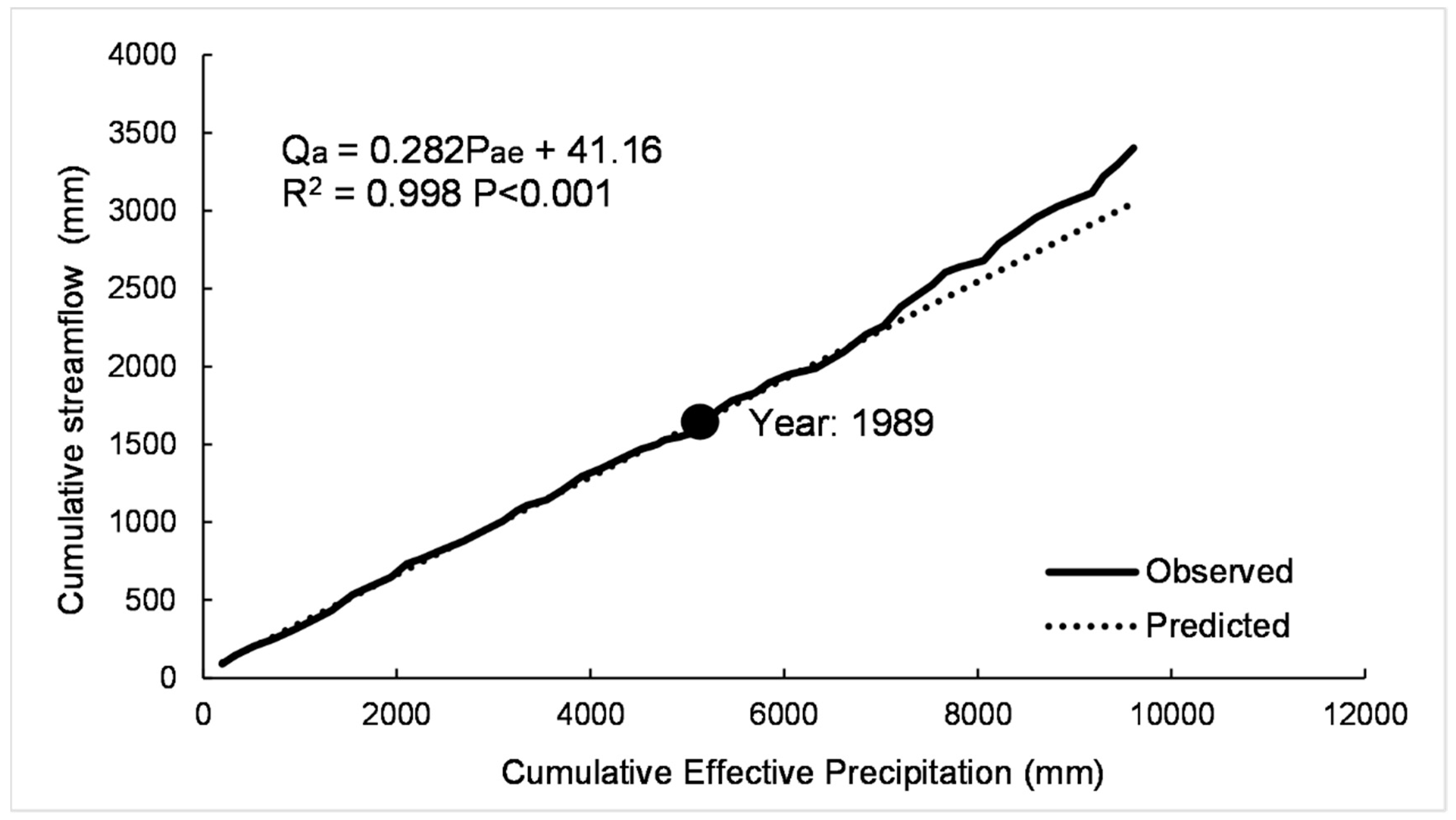
A breakpoint was identified on the MDMC, which plots cumulative effective precipitation (Pae) versus cumulative annual mean flow (Qa) (Figure 4). The observed cumulative Qa is greater than predicted after the break point, indicating that forest disturbance has led to an increase in Qa. The Pettitt break point test indicates that there is a statically significant regime shift in 1989, leading to the pre- and post-disturbance periods being defined as 1960 to 1989 and 1990 to 2012, respectively. Mann–Whitney U tests confirmed that the slopes of MDMCs before and after the break point were statistically different (p-value < 0.001). The break point coincides with the history of forest disturbance as at the end of 1989, the cumulative area disturbed is 80.4 km2 and the CECA is 12.4% (Figure 3).
Further calculations on the difference between observed and predicted Qa in the post-disturbance period show that forest change increased Q (∆Qf) by an average of 16.6 mm annually. In contrast, climate variability played a more minor role in streamflow alteration, i.e. the Qmean change attributed to climate (∆Qc) is 2.7 mm in the disturbance period (Table 4). As a result, the relative contribution of forest change to the total change in Q (Rf) was 86.2% while the relative contribution of climate variability (Rc) was 18.8%. As indicated, the breaking point was not determined visually from the MDMC, but rather statistically using the Pettitt break point test. As a result, the calculated ∆Qf and ∆Qc for an individual year fluctuates with large variations in climatic inputs (primarily P). There are some dry years, when the observed line dips below the predicted in Figure 3 and the ∆Qc is negative. However, over the entire disturbance period, the calculated ∆Qf and ∆Qc are both positive.
Overall, the effects of climate variability on streamflow were much lower than those from forest disturbance, indicating streamflow variations in the Deadman River watershed were mainly caused by cumulative forest disturbance.
The disturbance period was further divided into five sub-periods to examine the temporal role of forest disturbance and climate variability in streamflow. As shown in Table 4, the Rf and Rc to streamflow showed temporal variations. For example, with less forest disturbance, the Rf was lower in 1995–1999 than in the other periods.
3.3.2. Sensitivity-Based Method
Similar to MDMC, results from the sensitivity-based method show an overall increase in Qmean due to cumulative forest change. Here, the increases in Qmean attributed to cumulative forest disturbance and climate variability in the period 1990–2012 were an average of 10.8 and 8.9 mm respectively (Table 4). The Rf derived from the sensitivity-based method (86.2%) is lower than that from the MDMC (54.7%). As with MDMC, the ∆Qf and ∆Qc for an individual year (or selected period) will fluctuate depending on the climatic inputs for that time. For example, the MDMC method calculated ∆Qc −1.61 mm in the period 2000 – 2004, reflecting the lower than average P in four out of five years in that period. The effect of forest disturbance is much more consistent with ∆Qf greater than zero in all selected periods. So although the results for an individual year may fluctuate, on average across the whole disturbance period, the two methods clearly indicate that the cumulative forest disturbance played a dominant role in Qmean variation.
3.4. Separation of Effects Of Forest Disturbance and Climate Variability on High and Low Flows
The paired-year approach revealed that the cumulative forest disturbance consistently increased Q5% and Q95%. The average high flow in the reference period (1962–1989) is 8.07 m3s−1 increasing by 58% to 12.74 m3s−1 in the disturbance period (1990–2012) (Table 5), with a statistically significant p-value. Similarly, the cumulative forest disturbance increased the average low flow by 19% from 0.26 to 0.31 m3s−1. These results are consistent with those from the cross-correlation analysis that also showed a positive relationship between forest disturbance and high and low flows. So although there is some uncertainty introduced in the paired-year approach by inexact matching of climate variables in paired reference and disturbance years, the consistency with cross-correlation analysis strengthens the result.
4. Discussion
4.1. The Cumulative Effects of Forest Disturbance on Annual Mean Flow
In this study, cumulative forest disturbance has increased Qmean in the Deadman River watershed. Both the MDMC and sensitivity-based methods derived similar results, giving a more robust answer than one individual method. While the increase in Qmean is consistent with most other studies in the region with a similar climate [22,36,61], some have found no significant change with forest disturbance [23]. Zhang et al. [61] found no relationship between low CECA (<15%) and Qmean, indicating that there may be no effect on Qmean with lower levels of disturbance. In two large neighboring watersheds in British Columbia, Zhang and Wei [23] found contrasting responses after high levels of forest disturbance, with the Willow watershed showing a significant increase in Qmean while the Bowron did not. They attributed this to differences in topography, climate and the spatial arrangement of harvesting. This variability highlights that the cumulative effects of forest disturbance are likely watershed specific. Two recent global review papers investigated 162 large watersheds (>1000 km2) [9] and 252 small (<1000 km2) [4] watersheds. These reviews identified that watershed area, climate regime, and forest type are key factors that affect the hydrological response to cumulative forest disturbance. As such, caution must be used when extrapolating results from one location to another and from one time period to another.
4.2. Additive Effects of Cumulative Forest Disturbance and Climate Variability on Annual Mean Flow
Both cumulative forest disturbance and climate variability were found to increase Qmean in the disturbance period, meaning that their effects are additive as opposed to offsetting. Here, the term ‘additive’ signifies that both forest change and climate variability affect streamflow in the same positive direction, it does not imply a simple additive relationship between the two drivers. Complex interactions do exist as studies have shown the effect of disturbance on streamflow is less pronounced at very high levels of rainfall [9,62]. In the Deadman River watershed since 1989, the combined effect of cumulative forest disturbance and climate variability has increased Qmean by an average of 19.6 mm year−1. Of the other studies that have investigated the influence of both forest disturbance and climate in this region, all have found that forest disturbance has increased Qmean while the climate decreased Qmean [22,36,63,64]. For example, Wei and Zhang [22] found offsetting effect on Qmean of climate and forest disturbance in the Willow River watershed, as did Li et al. [36] in the Upper Similkameen River watershed. Zhang and Wei [65] found that forest disturbance increased Qmean by 48.4 mm year−1, while climatic variability offset this by decreasing Qmean by 35.5 mm year−1 in the Baker Creek watershed. Zhang [63] found that the Willow, Baker, Moffat, and Tulameen watersheds all had offsetting effects on Qmean of climate and forest disturbance.
This study is different, in that the MDMC and sensitivity analysis both found that climate has increased Qmean, resulting in an additive rather than offsetting effect on Qmean. Although most studies have found the climate in the interior of British Columbia to be getting drier, this depends on the period chosen, as illustrated in Zhang and Wei [65] where the influence of the Pacific Decadal Oscillation (PDO) affected the calculated climatic trend. Winkler et al. [8] found that the disturbance period in their study of the Upper Penticton Creek was wetter and cooler than the calibration period, and attributed this to the PDO. In the Deadman River watershed, time-trend analysis indicated that there was an increasing trend in annual Tmean and PET, leading to the expectation that climate variability would have decreased Qmean over the study period. Surprisingly, both the MDMC and sensitivity-based method showed that climate variability increased Qmean over the disturbance period. The nearby meteorological station ‘Kamloops A’ was used to confirm annual trends in P, Tmin, Tmax, and Tmean derived from the ClimateBC data. Additionally, more detailed time-trend analyses were conducted for the reference and disturbance periods separately (Figure S5). Results showed that Tmean increased significantly over the entire study period, but in contrast, Tmean has a decreasing trend over the disturbance period, with statistical insignificance. Unlike Tmean, P has an insignificant trend for all tested periods (Tables S4 and S5). Although the climate was getting drier over the entire period, there was no significant trend during the disturbance period. As a result, climate variability may have played a positive role in streamflow in the disturbance period. These findings also highlight the need to understand the temporal climate variability in the specific study watershed.
4.3. The Cumulative Effects of Forest Disturbance on High and Low Flows
Cross-correlation analysis showed a positive relationship between disturbance and both low and high flows. Similarly, the paired-year approach found that low and high flows increased significantly by 20% and 58% respectively in the disturbance period. The positive relationship of low and high flows to forest disturbance is consistent with most other studies of forest disturbance in neighboring areas [29,35,36]. In the Upper Penticton watershed, Winkler et al. [8] found that while Qmean increased by a small amount (5%) with disturbance, spring run-off (high flow) increased dramatically between 19% and29% and summer water yield (low flow) decreased by a similar magnitude. In a snow dominated regime such as the Deadman River watershed, forest disturbance likely results in more snow accumulation and earlier snow melt driven spring freshet [8,25], leading to an increase in high flow [29,36]. Synchronisation of snow pack melt [23] or increased quick flow [66] may also contribute to the increase in high flows. The increase in low flow with disturbance is likely due to a different mechanism than high flow. Summer low flows may be increased by the reduced ET side of the water balance equation, with lower growth removing less water from the soil, and consequently increasing recharge [67]. Increased throughfall, infiltration and snowpack accumulation associated with canopy removal can also increase soil moisture and recharge [68]. Winter harvesting practices in the area reduce the soil compaction and associated loss of recharge, however diversion associated with roads and skid trails can modify run-off pathways [26].
However, some studies in large watersheds show no or insignificant change to low flow with forest disturbance. For example, Zhang and Wei [23] investigated low and high flows in two large highly disturbed watersheds, finding that forest harvesting increased peak flows in one but not the other and found no significant changes on low flow. A study in the Canadian Boreal forest found that forest disturbance did not impact peak flow, but increased low flow [69]. Liu et al. [14] found contrasting responses to reforestation in two large watersheds in China with one showing significant and positive effects on low flows and the other not. Another study in subtropical China, found that deforestation increased both low and high flows [42]. Wilk et al. [70] found no changes in hydrology in the 12,100 km2 Nam Pong catchment in Thailand as forest cover was reduced from 80% to 27%. The influence of forest change on low flow depends upon factors such as soils, previous land uses, and climatic regime [30,31]. Soil properties such as porosity and organic matter content affect hydrological processes such as infiltration, surface and subsurface run-off, and can amplify or mute the effects of land use change [66]. For example, soils with a large holding capacity can dampen the effect of vegetation removal, while soil compaction and degradation may limit hydrological recovery with regeneration [31]. These contrary results highlight the watershed and region-specific nature of the effect of forest disturbance on high and low flows.
4.4. Management Implications
Our results show that Q5% increases with greater CECA, implying that forest harvesting increases high flows in this area. Consequently, if harvest rates are not limited, changes to the peak flow regime could result in undesirable alterations to riparian ecosystems and aquatic habitat [29,71]. Much of the BC interior is managed to a maximum logged CECA threshold of 20% to 30% [24] of the watershed area, which is intended to serve as a coarse filter to identify watersheds that may have impacts from harvesting [27]. Stednick [72] suggested that more than 20% of forest harvest in a watershed could lead to significant annual streamflow change. However, in our study, the cumulative effects of forest disturbance became apparent in the MDMC slope in 1989 at a CECA of 12.4%, indicating that the effects of forest disturbance and climate may begin to affect some watersheds at a much lower CECA than is managed for currently in BC. Water use allocations, environmental flow needs, and forest management all need to consider the long term trajectory of forest condition and climate, and their interactions.
5. Conclusions
This study assessed how two main drivers, cumulative forest cover change and climate variability, have influenced streamflow in the Deadman River watershed. In the period 1990–2012, overall the effects of cumulative forest disturbance and climate variability are additive, —both have increased Qmean. Forest disturbance increased Qmean by an average of 14 mm and climate variability increased it by 6 mm. Additionally, we found that forest disturbance increased low and high flows by 19% and 58% respectively. These insights provide an important contribution to the knowledge required for effective forest and watershed management under a changing climate.
Supplementary Materials
The following are available online at https://0-www-mdpi-com.brum.beds.ac.uk/1999-4907/10/2/196/s1. Figure S1: Average daily flow hydrograph of Deadman River watershed. Figure S2: Annual mean, low and high flows in the Deadman River watershed. Figure S3: Average annual daily average, maximum and miminum temperature in the Deadman River watershed. Figure S4: Annual precipitation, potential evapotranspiration and evapotranspiration in the Deadman River watershed. Figure S5: Average annual daily average, maximum and miminum temperature in the Deadman River watershed and the Kamloops A climate station. Table S1: Kendall tau tests between the hydrological variables and climate variables by season. Table S2: Canonical correlation analysis between hydrological variables and the set of climate variables. Table S3: Paired climate variables and hydrological variables in the paired-year analysis. Table S4: Trend analysis results for Kamloops A station data for seasonal and annual climatic variables over the reference and disturbance periods.Table S5: Trend analysis results for Deadman river watershed—level ClimateBC data for seasonal and annual climatic variables over the reference and disturbance periods.
Author Contributions
Conceptualization, K.G.-H., Q.L. and X.W.; Formal analysis, K.G.-H. and Q.L.; Funding acquisition, X.W.; Methodology, K.G.-H., Q.L. and X.W.; Supervision, X.W.; Validation, Q.L.; Writing—original draft, K.G.-H.; Writing—review & editing, Q.L. and X.W.
Funding
This research was funded by the Natural Sciences and Engineering Research Council of Canada (NSERC) Collaborative Research and Development Grant-Project (CRDPJ) entitled “The effects of reforestation on forest carbon and water coupling at multiple spatial scales”, grant number CRDPJ 485176-15.
Conflicts of Interest
The authors declare no conflicts of interest.
References
- Ellison, D.; Morris, C.E.; Locatelli, B.; Sheil, D.; Cohen, J.; Murdiyarso, D.; Gutierrez, V.; Noordwijk, M.V.; Creed, I.F.; Pokorny, J.; et al. Trees, forests and water: Cool insights for a hot world. Glob. Environ. Change 2017, 43, 51–61. [Google Scholar] [CrossRef] [Green Version]
- Wei, X.; Li, Q.; Zhang, M.; Giles-Hansen, K.; Liu, W.; Fan, H.; Wang, Y.; Zhou, G.; Piao, S.; Liu, S. Vegetation cover—Another dominant factor in determining global water resources in forested regions. Glob. Change Biol. 2018, 24, 786–795. [Google Scholar] [CrossRef] [PubMed]
- Wei, X.; Liu, W.; Zhou, P. Quantifying the Relative Contributions of Forest Change and Climatic Variability to Hydrology in Large Watersheds: A Critical Review of Research Methods. Water 2013, 5, 728–746. [Google Scholar] [CrossRef] [Green Version]
- Zhang, M.; Liu, N.; Harper, R.; Li, Q.; Liu, K.; Wei, X.; Ning, D.; Hou, Y.; Liu, S. A global review on hydrological responses to forest change across multiple spatial scales: Importance of scale, climate, forest type and hydrological regime. J. Hydrol. 2017, 546, 44–59. [Google Scholar] [CrossRef]
- Zhang, L.; Hickel, K.; Shao, Q. Predicting afforestation impacts on monthly streamflow using the DWBM model. Ecohydrology 2016. [Google Scholar] [CrossRef]
- Ford, C.R.; Laseter, S.H.; Swank, W.T.; Vose, J.M. Can forest management be used to sustain water-based ecosystem services in the face of climate change? Ecol. Appl. 2011, 21, 2049–2067. [Google Scholar] [CrossRef] [PubMed]
- Kelly, C.N.; McGuire, K.J.; Miniat, C.F.; Vose, J.M. Streamflow response to increasing precipitation extremes altered by forest management. Geophys. Res. Lett. 2016, 43, 3727–3736. [Google Scholar] [CrossRef] [Green Version]
- Winkler, R.; Spittlehouse, D.; Boon, S. Streamflow Response to Clearcut Logging on British Columbia’s Okanagan Plateau. Ecohydrology 2017. [Google Scholar] [CrossRef]
- Li, Q.; Wei, X.; Zhang, M.; Liu, W.; Fan, H.; Zhou, G.; Giles-Hansen, K.; Liu, S.; Wang, Y. Forest cover change and water yield in large forested watersheds: A global synthetic assessment. Ecohydrology 2017, 10. [Google Scholar] [CrossRef]
- Bosch, J.M.; Hewlett, J.D. A review of catchment experiments to determine the effect of vegetation changes on water yield and evapotranspiration. J. Hydrol. 1982, 55, 3–23. [Google Scholar] [CrossRef]
- Brown, A.E.; Zhang, L.; McMahon, T.A.; Wes tern, A.W.; Vertessy, R.A. A review of paired catchment studies for determining changes in water yield resulting from alterations in vegetation. J. Hydrol. 2005, 310, 28–61. [Google Scholar] [CrossRef]
- Forest and Water on a Changing Planet:Vulnerability, Adaptation and Governance Opportunities. A Global Assessment Report. In Proceedings of the IUFRO World Series, Vienna, Austria, 10 July 2018; p. 192.
- Dey, P.; Mishra, A. Separating the impacts of climate change and human activities on streamflow: A review of methodologies and critical assumptions. J. Hydrol. 2017, 548, 278–290. [Google Scholar] [CrossRef]
- Liu, W.; Wei, X.; Li, Q.; Fan, H.; Duan, H.; Wu, J.; Giles-Hansen, K.; Zhang, H. Hydrological recovery in two large forested watersheds of southeastern China: The importance of watershed properties in determining hydrological responses to reforestation. Hydrol. Earth Syst. Sci. 2016, 20, 4747–4756. [Google Scholar] [CrossRef]
- Ruiz-Perez, G.; Koch, J.; Manfreda, S.; Caylor, K.; Frances, F. Calibration of a parsimonious distributed ecohydrological daily model in a data scarce basin using exclusively the spatio-temporal variation of NDVI. Hydrol. Earth System Sci. 2017, 21, 6235–6251. [Google Scholar] [CrossRef]
- Mikkelson, K.M.; Maxwell, R.M.; Ferguson, I.; Stednick, J.D.; McCray, J.E.; Sharp, J.O. Mountain pine beetle infestation impacts: modeling water and energy budgets at the hill-slope scale. Ecohydrology 2013, 6, 64–72. [Google Scholar] [CrossRef]
- Penn, C.A.; Bearup, L.A.; Maxwell, R.M.; Clow, D.W. Numerical experiments to explain multiscale hydrological responses to mountain pine beetle tree mortality in a headwater watershed. Water Resour. Res. 2016, 52, 3143–3161. [Google Scholar] [CrossRef] [Green Version]
- Schnorbus, M.; Bennett, K.; Werner, A. Quantifying the water resource impacts of mountain pine beetle and associated salvage harvest operations across a range of watershed scales: Hydrologic modelling of the Fraser River Basin. In Information Report BC-X-423; Natural Resources Canada, Canadian Forest Service, Pacific Forestry Centre: Victoria, BC, Canada, 2010. [Google Scholar]
- White, J.C.; Wulder, M.A.; Hermosilla, T.; Coops, N.C.; Hobart, G.W. A nationwide annual characterization of 25years of forest disturbance and recovery for Canada using Landsat time series. Remote Sens. Environ. 2017, 194, 303–321. [Google Scholar] [CrossRef]
- Reid, L.M. Cumulative watershed effects and watershed analysis. In River Ecology and Management: Lessons from the Pacific Coastal Ecoregion; Naiman, R.J., Bilby, R.E., Eds.; Springer: New York, NY, USA, 1998; pp. 476–501. [Google Scholar]
- Schindler, D.W.; Donahue, W.F. An impending water crisis in Canada’s western prairie provinces. Proc. Natl. Acad. Sci. USA 2006, 103, 7210. [Google Scholar] [CrossRef] [PubMed]
- Wei, X.; Zhang, M. Quantifying streamflow change caused by forest disturbance at a large spatial scale: A single watershed study. Water Resour. Res. 2010, 46. [Google Scholar] [CrossRef] [Green Version]
- Zhang, M.; Wei, X. Contrasted hydrological responses to forest harvesting in two large neighbouring watersheds in snow hydrology dominant environment: implications for forest management and future forest hydrology studies. Hydrol. Process. 2014, 28, 6183–6195. [Google Scholar] [CrossRef]
- Winkler, R.; Boon, S. Revised Snow Recovery Estimates for Pine-dominated Forests in Interior British Columbia; Extension note 116; Ministry of Forests, Lands and Natural Resource Operations: Kamloops, BC, Canada, 2015.
- Winkler, R.D.; Moore, R.D.; Redding, T.E.; Spittlehouse, D.L.; Smerdon, B.D.; Carlyle-Moses, D.E. The Effects of Forest Disturbance on Hydrologic Processes and Watershed Response (Chapter 7). In Compendium of Forest Hydrology and Geomorphology in British Columbia; British Columbia: Victoria, BC, Canada, 2010. [Google Scholar]
- Moore, D.R.; Wondzell, S.M. Physical Hydrology and the Effects of Forest Harvesting in the Pacific Northwest: A Review. JAWRA 2005, 41, 763–784. [Google Scholar] [CrossRef]
- British Columbia Ministry of Forests. Forest Practices Code of British Columbia. In Coastal Watershed Assessment Procedure Guidebook (CWAP) and Interior Watershed Assessment Procedure Guidebook (IWAP); British Columbia Ministry of Forests: Victoria, BC, Canada, 1999. [Google Scholar]
- Jones, J.A.; Perkins, R.M. Extreme flood sensitivity to snow and forest harvest, western Cascades, Oregon, United States. Water Resour. Res. 2010, 46. [Google Scholar] [CrossRef] [Green Version]
- Zhang, M.; Wei, X. Alteration of flow regimes caused by large-scale forest disturbance: a case study from a large watershed in the interior of British Columbia, Canada. Ecohydrology 2014, 7, 544–556. [Google Scholar] [CrossRef]
- Liu, W.; Wei, X.; Liu, S.; Liu, Y.; Fan, H.; Zhang, M.; Yin, J.; Zhan, M. How do climate and forest changes affect long-term streamflow dynamics? A case study in the upper reach of Poyang River basin. Ecohydrology 2015, 8, 46–57. [Google Scholar] [CrossRef]
- Bruijnzeel, L.A. Hydrological functions of tropical forests: not seeing the soil for the trees? Agric. Ecosyst. Environ. 2004, 104, 185–228. [Google Scholar] [CrossRef]
- Ecoscape Environmental Consultants Ltd. Deadman River Sensitive Habitat Inventory and Mapping (SHIM)-2009–2011; Inventory Summary Report; Skeetchestn Indian Band: Kelowna, BC, Canada, 2012; p. 28. [Google Scholar]
- Walton, A. Provincial-Level Projection of the Current Mountain Pine Beetle Outbreak: Update of the Infestation Projection Based on the Provincial Aerial Overview Surveys of Forest Health Conducted from 1999 through 2012 and the BCMPB Model (Year 10). BC Forest Service, 2013. Available online: https://www.google.com.sg/url?sa=t&rct=j&q=&esrc=s&source=web&cd=1&ved=2ahUKEwjPw-Tvn8zgAhWDLqYKHdg5AnIQFjAAegQIARAC&url=https%3A%2F%2Fwww.for.gov.bc.ca%2Fftp%2Fhre%2Fexternal%2F!publish%2Fweb%2Fbcmpb%2Fyear10%2FBCMPB.v10.BeetleProjection.Update.pdf&usg=AOvVaw1l11YYPl_TOX7qhgj15tq1 (accessed on 11 January 2019).
- Wang, T.; Hamann, A.; Spittlehouse, D.; Carroll, C. Locally Downscaled and Spatially Customizable Climate Data for Historical and Future Periods for North America. PLoS ONE 2016, 11, e0156720. [Google Scholar] [CrossRef] [PubMed]
- Zhang, M.; Wei, X.; Li, Q. A quantitative assessment on the response of flow regimes to cumulative forest disturbances in large snow-dominated watersheds in the interior of British Columbia, Canada. Ecohydrology 2016, 9, 843–859. [Google Scholar] [CrossRef]
- Li, Q.; Wei, X.; Zhang, M.; Liu, W.; Giles-Hansen, K.; Wang, Y. The cumulative effects of forest disturbance and climate variability on streamflow components in a large forest-dominated watershed. J. Hydrol. 2018, 557, 448–459. [Google Scholar] [CrossRef]
- Lewis, D.; Huggard, D. A Model to Quantify Effects of Mountain Pine Beetle on Equivalent Clearcut Area. Streamline Watershed Manag. Bull. 2010, 13, 42–51. [Google Scholar]
- Axelson, J.N.; Alfaro, R.I.; Hawkes, B.C. Influence of fire and mountain pine beetle on the dynamics of lodgepole pine stands in British Columbia, Canada. For. Ecol. Manage. 2009, 257, 1874–1882. [Google Scholar] [CrossRef]
- Baker, E.H.; Painter, T.H.; Schneider, D.; Meddens, A.J.H.; Hicke, J.A.; Molotch, N.P. Quantifying insect-related forest mortality with the remote sensing of snow. Remote Sens. Environ. 2017, 188, 26–36. [Google Scholar] [CrossRef]
- R Core Team. R: A Language and Environment for Statistical Computing. R Foundation for Statistical Computing: Vienna, Austria, 2016. [Google Scholar]
- Hyndman, R.J.; Khandakar, Y. Automatic time series forecasting: the forecast package for R. J. Stat. Softw. 2008, 27, 1–22. [Google Scholar] [CrossRef]
- Liu, W.; Wei, X.; Fan, H.; Guo, X.; Liu, Y.; Zhang, M.; Li, Q. Response of flow regimes to deforestation and reforestation in a rain-dominated large watershed of subtropical China. Hydrol. Process. 2015, 29, 5003–5015. [Google Scholar] [CrossRef]
- Mann, H.B. Nonparametric Tests Against Trend. Econometrica 1945, 13, 245–259. [Google Scholar] [CrossRef]
- Kendall, M.G. Rank Correlation Methods; Oxford University Press: New York, NY, USA, 1975; p. 202. [Google Scholar]
- Déry, S.J.; Wood, E.F. Decreasing river discharge in northern Canada. Geophys. Res. Lett. 2005, 32. [Google Scholar] [CrossRef]
- Yue, S.; Pilon, P.; Phinney, B.; Cavadias, G. The influence of autocorrelation on the ability to detect trend in hydrological series. Hydrol. Process. 2002, 16, 1807–1829. [Google Scholar] [CrossRef]
- Razavi, S.; Vogel, R. Prewhitening of hydroclimatic time series? Implications for inferred change and variability across time scales. J. Hydrol. 2018, 557, 109–115. [Google Scholar] [CrossRef]
- Priestley, C.H.B.; Taylor, R.J. On the assessment of surface heat flux and evaporation using large-scale parameters. Mon. Weather Rev. 1972, 100, 81–82. [Google Scholar] [CrossRef]
- Hamon, W.R. Computation of Direct Runoff Amounts From Storm Rainfall. IAHS 1963, 63, 52–62. [Google Scholar]
- Lu, J.; Sun, G.; McNulty, S.G.; Amatya, D. A comparison of six potential evapotranspiration methods for regional use in the Southeastern United States. JAWRA 2005, 41, 621–633. [Google Scholar] [CrossRef]
- McMahon, T.A.; Peel, M.C.; Lowe, L.; Srikanthan, R.; McVicar, T.R. Estimating actual, potential, reference crop and pan evaporation using standard meteorological data: a pragmatic synthesis. Hydrol. Earth Syst. Sci. 2013, 17, 1331–1363. [Google Scholar] [CrossRef]
- Budyko, M.I. Climate and Life; Academic Press: London, UK, 1974; Volume 18. [Google Scholar]
- Zhang, L.; Hickel, K.; Dawes, W.R.; Chiew, F.H.S.; Western, A.W.; Briggs, P.R. A rational function approach for estimating mean annual evapotranspiration. Water Resour. Res. 2004, 40. [Google Scholar] [CrossRef] [Green Version]
- Yao, Y.; Cai, T.; Wei, X.; Zhang, M.; Ju, C. Effect of forest recovery on summer streamflow in small forested watersheds, Northeastern China. Hydrol. Process. 2012, 26, 1208–1214. [Google Scholar] [CrossRef]
- Pettitt, A.N. A Non-Parametric Approach to the Change-Point Problem. J. R. Stat. Soc. Ser. C Appl. Stat. 1979, 28, 126–135. [Google Scholar] [CrossRef]
- Li, Y.; Piao, S.; Li, L.Z.X.; Chen, A.; Wang, X.; Ciais, P.; Huang, L.; Lian, X.; Peng, S.; Zeng, Z.; et al. Divergent hydrological response to large-scale afforestation and vegetation greening in China. Sci. Adv. 2018, 4. [Google Scholar] [CrossRef] [PubMed]
- Koster, R.D.; Suarez, M.J. A Simple Framework for Examining the Interannual Variability of Land Surface Moisture Fluxes. J. Climate 1999, 12, 1911–1917. [Google Scholar] [CrossRef]
- Milly, P.C.D.; Dunne, K.A. Macroscale water fluxes 1. Quantifying errors in the estimation of basin mean precipitation. Water Resour. Res. 2002, 38, 1–14. [Google Scholar] [CrossRef]
- Serinaldi, F.; Kilsby, C.G.; Lombardo, F. Untenable nonstationarity: An assessment of the fitness for purpose of trend tests in hydrology. Adv. Water Resour. 2018, 111, 132–155. [Google Scholar] [CrossRef]
- Mikkelson, K.M.; Bearup, L.A.; Maxwell, R.M.; Stednick, J.D.; McCray, J.E.; Sharp, J.O. Bark beetle infestation impacts on nutrient cycling, water quality and interdependent hydrological effects. Biogeochemistry 2013, 115, 1–21. [Google Scholar] [CrossRef]
- Zhang, M.; Wei, X.; Li, Q. Do the hydrological responses to forest disturbances in large watersheds vary along climatic gradients in the interior of British Columbia, Canada? Ecohydrology 2017, 10, e1840. [Google Scholar] [CrossRef]
- Berghuijs Wouter, R.; Larsen Joshua, R.; van Emmerik Tim, H.M.; Woods Ross, A. A Global Assessment of Runoff Sensitivity to Changes in Precipitation, Potential Evaporation, and Other Factors. Water Resour. Res. 2017, 53, 8475–8486. [Google Scholar] [CrossRef] [Green Version]
- Zhang, M. The effects of cumulative forest disturbances on hydrology in the interior of British Columbia, Canada. Ph.D. Thesis, The University of British Columbia (Okanagan), Kelowna, BC, Canada, June 2013. [Google Scholar]
- Zhang, M.; Wei, X.; Sun, P.; Liu, S. The effect of forest harvesting and climatic variability on runoff in a large watershed: The case study in the Upper Minjiang River of Yangtze River basin. J. Hydrol. 2012, 464–465, 1–11. [Google Scholar] [CrossRef]
- Zhang, M.; Wei, X. The effects of cumulative forest disturbance on streamflow in a large watershed in the central interior of British Columbia, Canada. HESS 2012, 16, 2021–2034. [Google Scholar] [CrossRef] [Green Version]
- Roa-García, M.C.; Brown, S.; Schreier, H.; Lavkulich, L.M. The role of land use and soils in regulating water flow in small headwater catchments of the Andes. Water Resour. Res. 2011, 47. [Google Scholar] [CrossRef] [Green Version]
- Clark, K.L.; Skowronski, N.; Gallagher, M.; Renninger, H.; Schäfer, K. Effects of invasive insects and fire on forest energy exchange and evapotranspiration in the New Jersey pinelands. Agric. For. Meteorol. 2012, 166–167, 50–61. [Google Scholar] [CrossRef]
- Du, E.; Link, T.E.; Wei, L.; Marshall, J.D. Evaluating hydrologic effects of spatial and temporal patterns of forest canopy change using numerical modelling. Hydrol. Process. 2016, 30, 217–231. [Google Scholar] [CrossRef]
- Buttle, J.M.; Metcalfe, R.A. Boreal forest disturbance and streamflow response, northeastern Ontario. Can. J. Fish. Aquat. Sci. 2000, 57, 5–18. [Google Scholar] [CrossRef] [Green Version]
- Wilk, J.; Andersson, L.; Plermkamon, V. Hydrological impacts of forest conversion to agriculture in a large river basin in northeast Thailand. Hydrol. Process. 2001, 15, 2729–2748. [Google Scholar] [CrossRef]
- Chen, W.; Wei, X. Assessing the relations between aquatic habitat indicators and forest harvesting at watershed scale in the interior of British Columbia. For. Ecol. Manage. 2008, 256, 152–160. [Google Scholar] [CrossRef]
- Stednick, J.D. Monitoring the effects of timber harvest on annual water yield. J. Hydrol. 1996, 176, 79–95. [Google Scholar] [CrossRef]
Figure 1.
The location of watershed boundary, hydrometric station, stream network, forest logging, and mountain pine beetle (MPB) infestation of the Deadman River watershed, located in British Columbia, Canada.
Figure 1.
The location of watershed boundary, hydrometric station, stream network, forest logging, and mountain pine beetle (MPB) infestation of the Deadman River watershed, located in British Columbia, Canada.

Figure 2.
Equivalent clear-cut area (ECA) (%) since year of disturbance by mountain pine beetle (MPB).
Figure 2.
Equivalent clear-cut area (ECA) (%) since year of disturbance by mountain pine beetle (MPB).

Figure 3.
Annual area disturbed (km2) and Cumulative Equivalent clear-cut area (CECA) in percent (% of watershed area) by disturbance type and total in the Deadman River watershed from 1960 to 2012.
Figure 3.
Annual area disturbed (km2) and Cumulative Equivalent clear-cut area (CECA) in percent (% of watershed area) by disturbance type and total in the Deadman River watershed from 1960 to 2012.

Figure 4.
Modified Double Mass Curve (MDMC) of cumulative effective precipitation (Pae) versus cumulative annual mean flow (Qa) in the Deadman River watershed from 1960 to 2012. The ‘Predicted’ line is from the linear equation shown on the graph. The breakpoint is in 1989.
Figure 4.
Modified Double Mass Curve (MDMC) of cumulative effective precipitation (Pae) versus cumulative annual mean flow (Qa) in the Deadman River watershed from 1960 to 2012. The ‘Predicted’ line is from the linear equation shown on the graph. The breakpoint is in 1989.


Table 1.
Hydrological recovery and equivalent clear-cut area (ECA) for stands disturbed by wildfire or harvesting according to height in meters (m) of the leading tree species.
Table 1.
Hydrological recovery and equivalent clear-cut area (ECA) for stands disturbed by wildfire or harvesting according to height in meters (m) of the leading tree species.
| Height (m) | Hydrologic Recovery (%) | ECA (%) |
|---|---|---|
| 0 ≤ 3 | 0 | 100 |
| 3 ≤ 5 | 25 | 75 |
| 5 ≤ 7 | 50 | 50 |
| 7 ≤ 9 | 75 | 25 |
| >9 | 90 | 10 |
Table 2.
Time-trend analysis of hydro-meteorological variables in the Deadman River watershed from 1962 to 2012 (spring: March–May; summer: June–August; autumn: September–November; winter: December–February; Tmax is maximum daily annual temperature (°C); Tmin is minimum daily annual temperature (°C); Tmean is average daily annual temperature (°C); P is annual precipitation (mm); PET is potential evapotranspiration (mm); AET is actual evapotranspiration (mm); Qmean is annual mean flow (mm); Q95% is the low flow parameter; Q5% is the high flow parameter; tau is the z-statistic from the Mann–Kendall test indicating the direction of change of the variable; p-value is the level of significance from the Mann–Kendall test; and bolded italics indicate significant trends at a significance level of 0.05).
| Season | Tmax | Tmin | Tmean | P | PET | AET | Q5% | Q95% | Qmean | |
|---|---|---|---|---|---|---|---|---|---|---|
| Annual | tau | 0.19 | 0.25 | 0.23 | −0.02 | 0.25 | 0.06 | –0.04 | 0.24 | 0.01 |
| p-value | 0.05 | 0.01 | 0.01 | 0.87 | 0.01 | 0.55 | 0.73 | 0.02 | 0.95 | |
| Spring | tau | 0.08 | 0.18 | 0.15 | 0.21 | 0.17 | 0.25 | –0.01 | 0.05 | –0.06 |
| p-value | 0.41 | 0.05 | 0.11 | 0.02 | 0.08 | 0.01 | 0.91 | 0.59 | 0.55 | |
| Summer | tau | 0.09 | 0.25 | 0.13 | 0.04 | 0.16 | 0.08 | –0.08 | 0.11 | –0.01 |
| p-value | 0.35 | 0.01 | 0.17 | 0.68 | 0.09 | 0.42 | 0.45 | 0.29 | 0.96 | |
| Autumn | tau | 0.16 | 0.04 | 0.06 | 0.05 | 0.10 | 0.05 | 0.06 | 0.26 | 0.23 |
| p-value | 0.08 | 0.71 | 0.50 | 0.60 | 0.27 | 0.57 | 0.54 | 0.01 | 0.02 | |
| Winter | tau | 0.13 | 0.15 | 0.12 | –0.07 | 0.11 | 0.10 | 0.13 | 0.21 | 0.14 |
| p-value | 0.15 | 0.10 | 0.20 | 0.47 | 0.24 | 0.27 | 0.20 | 0.04 | 0.15 |
Table 3.
Cross-correlation results between the residuals of logged Autoregressive Integrated Moving Average (ARIMA) time series models for cumulative equivalent clear-cut area (CECA) and annual streamflow components in the Deadman River watershed from 1960 to 2012. The bold italicised coefficient value indicates that the model is significant at p-value = 0.05. Streamflow components include annual mean flow (Q), low flow (Q5%), and high flow (Q95%). The ARIMA model used is denoted by ln(p,d,q), where ln represents that the log of the data was taken prior to running the ARIMA model, p is the order of the auto-regressive model, d is the degree of differencing, and q is the order of moving-average chosen for the ARIMA model.
| Hydrological Variables | Cross-Correlation with CECA (Pre-Whitened Using ARIMA (2, 2, 1)) | ||
|---|---|---|---|
| ARIMA Model Used to Pre-Whiten | Coefficients | Lag | |
| Annual mean flow (Q) | (1, 3, 0) | 0.32 | 8 |
| High flow (Q5%) | (0, 1, 1) | 0.33 | 8 |
| Low flow (Q95%) | (0, 1, 2) | 0.32 | 4 |
Table 4.
Results from Modified Double Mass Curve (MDMC) and sensitivity-based analyses. Where ∆Q is the change in annual mean streamflow between the observed and predicted, ∆Qf is the difference in streamflow attributed to forest change, ∆Qc is the difference in streamflow attributed to climate variability, Rf and Rc are the relative contribution of forest change and climate variability to the total change in Q in that period expressed as a percentage. CECA is the average cumulative equivalent clear-cut area for the selected periods.
| Method | Selected Periods | ∆Q (mm) | ∆Qf (mm) | ∆Qc (mm) | Rf (%) | Rc (%) | CECA (%) |
|---|---|---|---|---|---|---|---|
| MDMC | 1990–1994 | 17.53 | 13.71 | 3.82 | 78.23 | 21.77 | 14.56 |
| 1995–1999 | 30.53 | 14.23 | 16.30 | 46.62 | 53.38 | 17.32 | |
| 2000–2004 | 3.02 | 4.63 | −1.61 | 74.18 | 25.82 | 18.21 | |
| 2005–2009 | 21.57 | 19.71 | 1.85 | 91.40 | 8.60 | 32.43 | |
| 2010–2012 | 27.12 | 34.20 | −7.08 | 82.85 | 17.15 | 51.67 | |
| 1990–2012 | 19.95 | 16.59 | 2.66 | 86.20 | 13.80 | 24.68 | |
| Sensitivity-based method | 1990–2012 | 19.65 | 10.75 | 8.90 | 54.70 | 45.30 | 24.68 |
Table 5.
Average high flow variable (Q5%) and low flow variable (Q95%) in the reference and disturbance periods using the paired-year approach.
Table 5.
Average high flow variable (Q5%) and low flow variable (Q95%) in the reference and disturbance periods using the paired-year approach.
| Flow (m3s−1) | Q5% | Q95% |
|---|---|---|
| Reference | 8.07 | 0.26 |
| Disturbance | 12.74 | 0.31 |
| Change (m3s−1) | 4.67 | 0.05 |
| Change (%) | 58% | 19% |
| p-value | <0.001 | <0.001 |
© 2019 by the authors. Licensee MDPI, Basel, Switzerland. This article is an open access article distributed under the terms and conditions of the Creative Commons Attribution (CC BY) license (http://creativecommons.org/licenses/by/4.0/).
Share and Cite
MDPI and ACS Style
Giles-Hansen, K.; Li, Q.; Wei, X. The Cumulative Effects of Forest Disturbance and Climate Variability on Streamflow in the Deadman River Watershed. Forests 2019, 10, 196. https://0-doi-org.brum.beds.ac.uk/10.3390/f10020196
AMA Style
Giles-Hansen K, Li Q, Wei X. The Cumulative Effects of Forest Disturbance and Climate Variability on Streamflow in the Deadman River Watershed. Forests. 2019; 10(2):196. https://0-doi-org.brum.beds.ac.uk/10.3390/f10020196
Chicago/Turabian StyleGiles-Hansen, Krysta, Qiang Li, and Xiaohua Wei. 2019. "The Cumulative Effects of Forest Disturbance and Climate Variability on Streamflow in the Deadman River Watershed" Forests 10, no. 2: 196. https://0-doi-org.brum.beds.ac.uk/10.3390/f10020196
Note that from the first issue of 2016, this journal uses article numbers instead of page numbers. See further details here.