Development of a Mixed-Effects Individual-Tree Basal Area Increment Model for Oaks (Quercus spp.) Considering Forest Structural Diversity

Abstract

In the context of uneven-aged mixed-species forest management, an individual-tree basal area increment model considering forest structural diversity was developed for oaks (Quercus spp.) using data collected from 11,860 observations in 845 sample plots from the 7th (2004), 8th (2009), and 9th (2014) Chinese National Forest Inventory in Hunan Province, south-central China. Since the data was longitudinal and had a nested structure, we used a linear mixed-effects approach to construct the model. We also used the variance function and an autocorrelation structure to describe within-plot heteroscedasticity and autocorrelation. Finally, the optimal mixed-effects model was determined based on the Akaike information criterion (AIC), Bayesian information criterion (BIC), log-likelihood (Loglik) and the likelihood ratio test (LRT). The results indicate that the reciprocal transformation of initial diameter at breast height (1/DBH), relative density index (RD), number of trees per hectare (NT), elevation (EL) and Gini coefficient (GC) had a significant impact on the individual-tree basal area increment. In comparison to the basic model developed using least absolute shrinkage and selection operator (LASSO) regression, the mixed-effects model performance was greatly improved. In addition, we observed that the heteroscedasticity was successfully removed by the exponent function and autocorrelation was significantly corrected by AR(1). Our final model also indicated that forest structural diversity significantly affected tree growth and hence should not be neglected. We hope that our final model will contribute to the scientific management of oak-dominated forests.

1. Introduction

The more than 500 extant species of oak (Quercus spp.) are widely distributed across the Northern Hemisphere, including Mesoamerica [1,2]. Oak-dominated forests are of great ecological and economical importance [3,4]. For instance, oaks are extensively used in soil and water conservation and restoration efforts since they have strong, adventitious root systems and exhibit a high tolerance to waterlogging [5,6,7]. Additionally, oaks are well adapted to fire and hence are frequently used for constructing forest fire belts [8]. Oaks also play an important role in maintaining biodiversity. For instance, Caprio and Ellena [9] reported that the retention of native oaks is the key factor for the conservation of winter bird diversity in local deciduous woods. In addition to the ecological functions, oak timber is distinguished for its great strength, durability and beauty [10]. As a high-grade material, oak is widely used in shipbuilding and in the manufacture of furniture, sports equipment and flooring [11].

China contains approximately 51 oak species, which are widely distributed throughout the country’s mountainous regions [12,13]. According to the 8th Chinese National Forest Inventory (CNFI), oak-dominated forests cover 16.72 million hm², accounting for 10.15% of the total forest area. Stocking is 1.294 billion m³, representing 8.76% of the total stocking in China [14]. A total of 96.29% of the oak-dominated forests in China are degraded secondary natural forests. They have historically experienced extensive disturbance, and many are almost coppice forests of very poor quality. For instance, the average stocking per hectare of oak-dominated forests in China is about 77.39 m³, while in Germany it is 305 m³ per hectare [15]. Therefore, it is urgent to manage these degraded forests in a sustainable way to improve their ecological and economic value.

The prediction of future stand development under different management scenarios is of great importance to inform forest management. Forest growth and yield models are an effective tool to provide such information [16,17]. Forest growth and yield models can be divided into three types, namely whole-stand growth models, size-class models and individual-tree models [18,19,20,21]. Almost all oak-dominated forests are uneven-aged mixed-species forests, and more detailed information is required to formulate management strategies for them. Under these circumstances, a whole-stand growth model, which is specifically produced for single-tree species plantations, is not appropriate [18]. Although size class models have been documented to model forest dynamics for uneven-aged mixed-species forests, they cannot provide the information required for individual trees. In China, close-to-nature forest management with a single tree selective cutting system has been widely adopted for the management of uneven-aged mixed-species forests [22]. This single-tree selective cutting system requires predictive information at the level of the individual trees. Fortunately, individual-tree models, which use single trees as the basic modeling unit, have the special ability to predict individual tree growth under a complex combination of species mixtures, stand structures, and silvicultural practices [23,24,25].

As an important component of individual-tree models, individual-tree basal area increment models are generally expressed as a linear function of tree size, competition pressures, and site conditions [26,27,28,29]. In China, individual-tree basal area increment models have been developed for many tree species, e.g., red pine (Pinus koraiensis Sieb. et Zucc.) [30], China fir (Cunninghamia lanceolata (Lamb.) Hook.) [31], and linden (Tilia tuan Szyszyl.) [32]. Unfortunately, there is no individual-tree basal area increment model for oak species in China. Additionally, forest structural diversity, an important part of biological diversity, has been extensively documented to affect forest growth and productivity [33,34]. For instance, Lei et al. [35] selected tree species, tree size, and height diversity indices to represent structural diversity and found that forest structural diversity had a significant positive effect on net growth and survivor growth. However, only a few studies have included forest structural diversity in forest growth and yield models.

The traditional regression analysis using ordinary least square regression (OLS) is the most commonly used method to develop individual-tree models [36,37]. In principle, the successful use of OLS requires that the data should satisfy the following statistical assumptions: independence of observations, and normally distributed residuals with equal variance of the residuals [38,39,40]. However, forestry data usually has the characteristic of a hierarchical stochastic structure because of the repeated measurements of the same sampling units and the nested structure of the sampling units [41,42]. This feature of forestry data violates these assumptions and using OLS in such a situation could result in biased estimations [42,43].

Mixed-effects models provide an efficient means to deal with longitudinal and nested data [44,45]. They contain both fixed effects parameters and random effects parameters. Fixed effects parameters account for covariate or treatment effects as in traditional regression, while random effects parameters explain the different sources of stochastic variability [46,47,48]. Mixed-effects models are therefore extensively used in forestry, such as diameter–height models [49,50], crown models [51,52], self-thinning models [53,54,55], and growth models [56,57].

In this study, the main objective was to develop a linear mixed-effects individual-tree basal area increment model for oaks in a degraded natural secondary forest in Hunan Province, south-central China. We hypothesized that the introduction of forest structural diversity and random effects would significantly improve model performance and we also hope our model will contribute to forest management strategies by predicting forest dynamics under different management scenarios.

2. Materials and Methods

2.1. Data and Pre-Analysis

According to the requirements of modeling data, 11,860 observations of 845 sample plots were selected from 6615 sample plots of the 7th (2004), 8th (2009), and 9th (2014) CNFI in Hunan Province, south-central China. The 0.067 ha square sample plots were systematically distributed in a grid of 4 × 8 km in Hunan Province, south-central China (Figure 1). At each sample plot, both individual-tree and plot information was recorded. The individual-tree information comprised tree species and diameter at breast height. Unfortunately, oaks were not identified to species level. Plot information included elevation, aspect, slope, soil type, soil depth, canopy closure, number of trees, dominant tree species, and forest types.

We randomly divided the data into two datasets, with 80% of the data used for model fitting (9739 observations from 676 sample plots) and the other 20% for model validation (2121 observations from 169 sample plots).

2.2. Methods

2.2.1. Development of Basic Model

The individual-tree basal area increment (BAI) can be described as a function of tree size (SIZE), competition pressures (COMP) and site conditions (SITE) in a stand [26,56,58,59]. We also considered the effects of forest structural diversity (DIVE) on BAI. Strictly speaking, structural diversity includes three categories—tree species diversity, tree size diversity, and tree position diversity. Unfortunately, due to the limited coordinate information available in the data, only tree species diversity and tree size diversity were considered. The relationship is expressed as follows:

BAI = SIZE + COMP + SITE + DIVE

(1)

The following independent variables were evaluated in our study:

(1)

Tree size effects: initial DBH, square of initial DBH (DBH²), reciprocal transformation of initial DBH (1/DBH) and natural logarithm of initial DBH (logDBH).

(2)

Competition pressures effects: number of trees per hectare (NT), stand basal area per hectare (BA), the sum of the basal area (m²/ha) in trees with DBHs larger than the subject tree’s DBH (BAL), the ratio of BAL and DBH (BAL/DBH), and the relative density index (RD = DBH/QMD).

(3)

Site conditions effects: elevation (EL), slope (SL) and aspect (ASP). Additionally, slope and aspect were combined using Stage’s transformation, i.e., SLCos = SL × cos(ASP), SLSin = SL × sin(ASP) [60].

(4)

Structural diversity effects: 1) tree species diversity: the Shannon–Wiener index (SHI), Pielou index (PI) and Simpson’s index (SII); 2) tree size diversity: the Gini coefficient (GC) and the standard deviation of the DBHs (SDDBH) [61].

$$\mathrm{SHI}=-{{\displaystyle \sum }}_{i=1}^{n}pi\ln \left(pi\right)$$

(2)

where $p_i$ is the proportion of basal areas in the ith species.

$$\mathrm{PI}=\frac{SHI}{\ln \left(S\right)}$$

(3)

where SHI is the Shannon–Wiener index and S is the total number of species in a sample, across all samples in a dataset.

$$\mathrm{SII}=1-{{\displaystyle \sum }}_{i=1}^n{p}_i^2$$

(4)

where $p_i$ is the proportion of basal areas in the ith species and n is the number of species observed.

$$\mathrm{GC}=\frac{{{\displaystyle \sum }}_{t=1}^n\left(2t-n-1\right)b{a}_t}{{{\displaystyle \sum }}_{t=1}^{n}b{a}_t\left(n-1\right)}$$

(5)

where ba_t is basal area for the tree in rank t (m²/ha) and t is the rank of a tree in order from 1, …, n.

Each of these variables has been documented to have a significant effect on individual-tree basal area increment. All variables used in the model development and their detailed descriptions are provided in

Table 1. Descriptive statistics for the candidate variables used in the model.

Variables	Min.	Max.	Mean	S.D.
DBH(cm)	5.0	65.7	9.76	5.39
NT	59	3402	1414	637
BA	0.38	53.31	13.83	8.45
BAL	0	3.56	0.67	0.50
QMD(cm)	5.9	29.2	11.1	3.2
EL(m)	5	1610	563.6	360.3
SL(per)	0	60	31.1	10.5
SHI	0.06	2.41	1.18	0.48
PI	0.0014	0.0525	0.0269	0.0111
SII	0.0196	0.8929	0.5606	0.2122
GC	0.1240	0.8202	0.4207	0.1029
SDDBH(cm)	0.7959	17.6867	4.3717	2.2605
iDBH(cm)	0.1	9.6	2.0	1.5

¹ DBH: initial DBH, NT: number of trees per hectare, BA: stand basal area per hectare, BAL: the sum of the basal area (m²/ha) in trees with DBHs larger than the subject tree’s DBH, QMD: quadratic mean DBH, EL: elevation, SL: slope, SHI: Shannon–Wiener index, PI: Pielou index, SII: Simpson’s index, GC: Gini coefficient, SDDBH: standard deviation of the DBHs, iDBH: diameter increment for five years, S.D.: standard deviation, Min.: minimum, Max.: maximum.

.

Different forms of dependent variables can result in different model performances [26,62,63]. The most frequently used dependent variables are the diameter increment (DBH₂ - DBH, in which DBH₂ denotes the DBH measured after a 5-year growth), squared diameter increment (DDS = ${\mathrm{DBH}}_2^2$ − DBH²), squared diameter increment plus a constant value of one (DDS + 1), and the natural logarithmic transformation of each [25,47,62]. These potential dependent variables were evaluated using the following lack-of-fit statistics, i.e., absolute bias (Bias), root mean square error (RMSE), and the coefficient of determination (R²). Additionally, residual plots were also produced to inspect the homogeneity of the variance and normality of the residuals. After comparing and testing these dependent variables, log(DDS + 1) was selected as the dependent variable for our basal area increment model since it performed best in terms of the normality and homogeneity of the residuals, and lack-of-fit statistics. Similar results were also reported by Calama and Montero [47], Adame et al. [63] and Lhotka and Loewenstein [25].

In this study, the basic individual-tree basal area increment model was developed by least absolute shrinkage and selection operator (LASSO) regression. The R package used for LASSO regression was glmnet [64]. For this method, the λ tuning parameter was determined by cross-validation using the fitting data with the mean square error as the criterion to obtain the candidate model. In order to check for multicollinearity amongst the variables, the variance inflation factor (VIF) was calculated. All variables with a VIF larger than 5 were removed to minimize overfitting [47,52,65]. Additionally, the relative importance refers to the quantification of an individual regressor’s contribution to a multiple regression model. In order to examine the relative effects of independent variables entering the final basic model, we calculated the relative importance values using the R Package “relaimpo”.

2.2.2. Development of Linear Mixed-Effects Model

Linear Mixed-Effects Model

Since our data was longitudinal (repeated measurement for each tree) and had a nested structure (tree nested within sample plots), we used a linear mixed-effects approach using sample plot as a random effect to produce our individual-tree basal area increment model. The general form of a linear mixed-effects model is as follows:

$$\begin{array}{c}{y}_i=x_i\mathsf{\beta }+z_i{b}_i+e_i\\ b_i~\mathrm{N}(0,{\sigma }^2)\\ e_i~\mathrm{N}(0,R_i)\end{array}$$

(6)

where $y_i$ represents the vector of the observations for the dependent variable, $x_i$ is a design matrix including covariates and derivative terms associated with fixed effects parameters, β is the vector of fixed parameters, $z_i$ is a design matrix for the random effects, and $b_i$ is the vector of random parameters. $e_i$ is error term, and $R_i$ is a positive definite variance–covariance matrix for the error term which includes the variance and correlation.

Construction of Parameter Effects

The parameters are divided into mixed-effects and fixed effects parameters. This is important when developing the mixed-effects model. In this study, all possible combinations were fitted and then the best combination with convergence was selected according to the Akaike information criterion (AIC), Bayesian information criterion (BIC), log-likelihood (Loglik) and the likelihood ratio test (LRT) [66,67]. The AIC, BIC and LRT are defined as follows:

$$\mathrm{AIC}=-2\mathrm{Loglik}+2\mathrm{d}$$

(7)

$$\mathrm{BIC}=-2\mathrm{Loglik}+\mathrm{dln}\left(\mathrm{n}\right)$$

(8)

$$\mathrm{LRT}=2\left[\log \left(L_2\right)-\log \left(L_1\right)\right]$$

(9)

where d is the number of estimated parameters of the model (including the intercept), n is the number of observations, and L₁ and L₂ are the likelihood value of different models.

Determination of Random Effects Variance–Covariance Structure

The variance–covariance matrices for the random effects are common to all sample plots. These matrices account for the variability between sample plots. In this study, we selected three structures to describe the random effects variance–covariance matrix. They were a diagonal matrix, a compound symmetry and general positive-definite matrix. The hypothetical 3 × 3 variance–covariance matrices are shown in Equations (10–12).

$$\mathrm{Diagonal}\mathrm{matrix}=\left[\begin{array}{ccc}{\sigma }_{b_1}^2& 0& 0\\ 0& {\sigma }_{b_2}^2& 0\\ 0& 0& {\sigma }_{b_3}^2\end{array}\right]$$

(10)

$$\mathrm{Compound}\mathrm{symmetry}=\left[\begin{array}{ccc}{\sigma }_{b_1}^2+{\sigma }^2& {\sigma }_1^2& {\sigma }_1^2\\ {\sigma }_1^2& {\sigma }_{b_1}^2+{\sigma }^2& {\sigma }_1^2\\ {\sigma }_1^2& {\sigma }_1^2& {\sigma }_{b_1}^2+{\sigma }^2\end{array}\right]$$

(11)

$$\mathrm{General}\mathrm{positive}\text{-}\mathrm{definite}\mathrm{matrix}=\left[\begin{array}{ccc}{\sigma }_{b_1}^2& {\sigma }_{b2b1}^2& {\sigma }_{b3b1}^2\\ {\sigma }_{b1b2}^2& {\sigma }_{b_2}^2& {\sigma }_{b3b2}^2\\ {\sigma }_{b1b3}^2& {\sigma }_{b2b3}^2& {\sigma }_{b_3}^2\end{array}\right]$$

(12)

where ${\sigma }_{b_u}^2$ (u = 1, 2, 3) is the variance in the $b_u$th random effect, and ${\sigma }_{b_u{b}_v}^2$ (u,v = 1, 2, 3, u ≠ v) is the covariance between the $b_u$th and the $b_v$th random effects, intercepting at ${\sigma }_{b_u{b}_v}^2$ = ${\sigma }_{b_v{b}_u}^2$.

Determining the Matrix of $R_i$

Heteroscedasticity and autocorrelation should be corrected when performing a regression analysis; if they are not, the computed standard errors and estimation interval will be incorrect, which will result in spurious regression problems [56,65]. Because the modeling data in this study was obtained from repeated measurements, the heteroscedasticity and autocorrelation of $R_i$ should be addressed [68]. The heteroscedasticity could be observed through the residual plot and quantile–quantile (QQ) plot. Additionally, we also conducted the Breusch–Pagan test to detect heteroscedasticity using the R Package “lmtest.” Because our data was of a longitudinal structure, i.e., two measurement periods, autocorrelation might have occurred. We therefore performed the Durbin–Watson test to investigate the autocorrelation using the R Package “car.” If there were heteroscedasticity and autocorrelation, we could introduce variance functions and autocorrelation structures to remove the heteroscedasticity of the residuals and correct autocorrelation among the observed values for the same tree obtained in different growth periods. The $R_i$ was written as follows [69]:

$$R_i={\sigma }^2{G}_i^{0.5}{\Gamma }_i{G}_i^{0.5}$$

(13)

where ${\sigma }^2$ is a scaling factor which is equal to the residual variance of the developed model, $G_i$ is a diagonal matrix which describes the heteroscedasticity and ${\Gamma }_i$ is a matrix showing the autocorrelation structure of errors.

Three different variance functions, i.e., the exponential function (Equation (14)), the power function (Equation (15)) and the constant plus power function (Equation (16)), were tested to remove heteroscedasticity [70].

$$\mathrm{varExp}(e_i)={\sigma }^2\exp \left(2\mathsf{\alpha }{u}_i\right)$$

(14)

$$\mathrm{varPower}(e_i)={\sigma }^2\exp \left(u_i^{2\alpha }\right)$$

(15)

$$\mathrm{varConstPower}\left(e_i\right)={\sigma }^2{\left(\mathsf{\alpha }+u_i^{\beta }\right)}^2$$

(16)

where $u_i$ is the estimated value based on fixed parameters of the linear mixed-effects model and α, β are estimated parameters of variance functions.

A first-order autoregressive structure (AR(1)), the compound symmetry structure (CS), and a combination of first-order autoregressive and moving average structures (ARMA(1,1)) were selected to correct autocorrelation [70]. The Equations (17)–(19) are the detailed matrix forms.

$$\mathrm{AR}(1)={\sigma }^2\left[\begin{array}{ccc}1& \rho & {\rho }^2\\ \rho & 1& \rho \\ {\rho }^2& \rho & 1\end{array}\right]$$

(17)

$$\mathrm{CS}=\left[\begin{array}{ccc}{\sigma }^2+{\sigma }_1& {\sigma }_1& {\sigma }_1\\ {\sigma }_1& {\sigma }^2+{\sigma }_1& {\sigma }_1\\ {\sigma }_1& {\sigma }_1& {\sigma }^2+{\sigma }_1\end{array}\right]$$

(18)

$$\mathrm{ARMA}(1,1)={\sigma }^2\left[\begin{array}{ccc}1& \upsilon & \upsilon \rho \\ \upsilon & 1& \upsilon \\ \upsilon \rho & \upsilon & 1\end{array}\right]$$

(19)

where $\rho$ is the autoregressive parameter, $\upsilon$ is a moving average component and ${\sigma }^2$ is the residual variance.

2.2.3. Random Parameters Prediction

The random parameters in Equation (20) were predicted using the best linear unbiased predictor (EBLUP) [46,71]:

$${\widehat{b}}_i\approx \widehat{D}{\widehat{Z}}_i^T{\left({\widehat{Z}}_i\widehat{\mathrm{D}}{\widehat{Z}}_i^T+{\widehat{R}}_i\right)}^{-1}{\widehat{e}}_i$$

(20)

where ${\widehat{b}}_i$ is a vector of random effects parameters of sample plots; $\widehat{D}$ is the m × m variance–covariance matrix for random effects (m is the number of random effects parameters);${\widehat{Z}}_i$ is the design matrix for the random effects parameters for the observations; ${\widehat{e}}_i$ is the residual vector whose components are given by the difference between the observations of individual-tree basal increment and predicted values from the mixed-effects model with only the fixed effects.

2.2.4. Model Prediction and Evaluation

As stated in our data and pre-analysis section, 20% of the plot data was used for model prediction. Using a mixed-effects model for prediction, two different predictive situations can be considered, i.e., the population average (PA) response, and the subject-specific (SS) response [47,67,72].

(a)

Population average responses (also termed marginal mean responses) are predicted using only the fixed effects part of a mixed-effects model if no additional information on random effects is available [47,72]. In this case, the expected value of the EBLUP’s for the random effects are zeroes, and the population average responses could hence be expressed as $\mathrm{E}\left(\mathrm{y}\right)=\mathrm{X}\mathsf{\beta }$.

(b)

Subject-specific responses (also called conditional mean responses) can be obtained using both fixed effects part and random effects part of a mixed-effects model, when the random parameters vector b can be predicted [47,65]. The subject-specific responses can be written as $\mathrm{E}\left(\mathrm{y}|\mathrm{b}\right)=\mathrm{X}\mathsf{\beta }+\mathrm{Zb}$. In this study, the random parameters for the evaluation data (the 20% of plot data) was predicted using the same method in Section 2.2.3.

2.2.5. Evaluated Statistics Indicator

In order to assess the predictive ability of the linear mixed-effects individual-tree basal area increment model, three lack-of-fit statistics were computed: the coefficient of determination (R²) (Equation (21)), absolute bias (Bias) (Equation (22)) and root mean square error (RMSE) (Equation (23)) [63,65].

$$R^2=1-\frac{{{\displaystyle \sum }}_{i=1}^n{(ob{j}_i-es{t}_i)}^2}{{{\displaystyle \sum }}_{i=1}^n{(ob{j}_i-{\overline{obj}}_i)}^2}$$

(21)

$$\mathrm{Bias}=\frac{{{\displaystyle \sum }}_{i=1}^n\left|\left(ob{j}_i-es{t}_i\right)\right|}{N}$$

(22)

$$\mathrm{RMSE}=\sqrt{\frac{{{\displaystyle \sum }}_{i=1}^n{\left(ob{j}_i-es{t}_i\right)}^2}{N-1}}$$

(23)

where $ob{j}_i$ is the observed value, $es{t}_i$ is the estimated value, ${\overline{obj}}_i$ is mean observed value, and N is the number of observations.

3. Results

3.1. Basic Model

The basic model using LASSO regression originally had nine independent variables. The tuning parameter λ, obtained by cross-validation, was 3.208 × 10⁻³. To avoid over overfitting and multicollinearity, we eliminated the variables of the candidate model with VIF > 5. This left 1/DBH, RD, NT, EL and GC to be entered into our basic model. Equation (24) was determined as our final basic model, to which random effects would be added to produce our linear mixed-effects individual-tree basal area increment model. The parameter estimates and their statistical description are shown in

Table 2. Statistical analysis results of variables of the individual-tree basal area increment model for oaks.

Variable	Parameters	Standard Deviation	t-Test	p Value	VIF
Intercept	1.878	0.04045	46.424	<0.001	-
1/DBH	−2.389	0.1389	−17.202	<0.001	3.19
RD	0.3208	0.01588	20.202	<0.001	3.09
NT	−0.0001327	0.000005652	−23.482	<0.001	1.13
EL	−0.0002252	0.00001044	−21.565	<0.001	1.23
GC	−0.1620	0.03856	−4.202	<0.001	1.37
AIC = 6317.446
BIC = 6367.733
Loglik = −3151.723

¹ VIF: variance inflation factor, AIC: Akaike information criterion, BIC: Bayesian information criterion, Loglik: log-likelihood.

.

$$\log (\mathrm{DDS}+1)={\mathsf{\beta }}_1 +{\mathsf{\beta }}_{2}1/\mathrm{DBH}+{\mathsf{\beta }}_3\mathrm{RD}+{\mathsf{\beta }}_4\mathrm{NT}+{\mathsf{\beta }}_5\mathrm{EL}+{\mathsf{\beta }}_6\mathrm{GC}+e_i$$

(24)

The residual plot and quantile–quantile (QQ) plot of the basic model (Equation (24)) are presented in Figure 2. Visually, the residuals were normally distributed with no pronounced heteroscedasticity. However, the Breusch–Pagan test indicated a heteroscedasticity of the residuals (p < 0.001). Additionally, the Durbin–Watson test indicated an autocorrelation (p < 0.001).

3.2. Linear Mixed-Effects Model

3.2.1. Random Parameter Effects

There are 63 ($C_6^1$ + $C_6^2$ + $C_6^3$ + $C_6^4$ + $C_6^5$ + $C_6^6$ = 63) potential different combinations of random effects for Equation (24) while considering all independent variables and the intercept in the basic model. A total of 49 combinations reached convergence when fitted to the data. Amongst these 49 mixed-effects models, Equation (25) yielded the smallest AIC (4836.349) and BIC (4994.392) and largest LogLik (-2396.174). In addition, the LRT also indicated the best performance of Equation (25). Equation (25) was the resulting mixed-effects model.

$$\begin{array}{c}\log (\mathrm{DDS}+1)=({\mathsf{\beta }}_1+{\mathrm{b}}_1)+\left({\mathsf{\beta }}_2+{\mathrm{b}}_2\right)1/\mathrm{DBH}+\left({\mathsf{\beta }}_3+{\mathrm{b}}_3\right)\mathrm{RD}+\left({\mathsf{\beta }}_4+{\mathrm{b}}_4\right)\mathrm{NT}+{\mathsf{\beta }}_5\mathrm{EL}+\\ \left({\mathsf{\beta }}_6+{\mathrm{b}}_5\right)\mathrm{GC}+e_i\end{array}$$

(25)

where ${\beta }_1$–${\beta }_6$ are the fixed effects parameters, and $b_1$–$b_5$ are the random effects parameters.

3.2.2. Random Effects Variance–Covariance Structure

The three different random effects variance–covariance structures, i.e., a diagonal matrix, a compound symmetry and general positive-definite matrix, were introduced to Equation (25), respectively, and their performances were compared. The general positive-definite matrix showed the best performance in terms of AIC, BIC, Loglik and LRT (

Table 3. The lack-of-fit statistics of the linear mixed-effects individual-tree basal area increment model using the three random effects variance–covariance structures.

Structures	AIC	BIC	LogLik	LRT	p
general positive-definite matrix	4836.349	4994.392	−2396.174
compound symmetry	5203.669	5268.323	−2592.834	393.3197	<0.001
diagonal matrix	4936.501	5022.707	−2456.251	120.1525	<0.001

). Therefore, the model with general positive-definite matrix was selected for our linear mixed-effects individual-tree basal area increment model.

3.2.3. Error Variance–Covariance Structure

We used three variance functions to remove the heteroscedasticity of the residuals and their performances were compared in terms of AIC, BIC, Loglik and LRT. The results showed that the mixed-effects models with the variance function exhibited better performance than the one without considering the variance function (

Table 4. The lack-of-fit statistics of the linear mixed-effects individual-tree basal area increment model using different error variance–covariance structures.

Model	Variance Function	Correlation Structure	AIC	BIC	LogLik	LRT	p
(1)	No	Independent	4836.349	4994.392	-2396.174
(2)	ConstPower	Independent	Nonconvergence
(3)	Power	Independent	4788.77	4953.997	-2371.385	49.5789 a	<0.001
(4)	Exponent	Independent	4780.131	4945.358	-2367.065	58.21805 a	<0.001
(5)	Exponent	CS	Nonconvergence
(6)	Exponent	AR(1)	4705.766	4878.177	-2328.883	76.3650 b	<0.001
(7)	Exponent	ARMA(1,1)	Nonconvergence

¹ CS: compound symmetry structure, AR(1): A first-order autoregressive structure, ARMA(1,1): a combination of first-order autoregressive and moving average structures; ^a Likelihood ratio is calculated with respect to model (1); ^b Likelihood ratio is calculated with respect to model (4).

). Performance also differed amongst the mixed-effects models with different variance functions. According to AIC, BIC, Loglik and LRT, the exponent function was determined as the best variance function.

The three correlation structures, i.e., AR(1), ARMA(1,1) and CS, were then used to correct the autocorrelation. According to the AIC, BIC, Loglik and LRT, AR(1) performed the best and hence was selected as the best autocorrelation structure for our mixed-effects model.

3.2.4. Final Form of the Linear Mixed-Effects Individual-Tree Basal Area Increment Model

After the determination of parameter effects, random effects variance–covariance structure and error variance–covariance structure, the final form of the linear mixed-effects individual-tree basal area increment model for oaks in Hunan Province, south-central China, was proposed in Equation (26) and Equation (27). The statistical analysis results of variables of the final mixed-effects model for oaks are shown in

Table 5. Statistical analysis results of variables of the linear mixed-effects individual-tree basal area increment model for oaks.

Variable	Fixed Effects Parameters	Standard Deviation	t-Test	p Value
Intercept	2.0435	0.0621	32.9262	<0.001
1/DBH	−2.8339	0.2019	−14.0361	<0.001
RD	0.2826	0.0200	14.0951	<0.001
NT	−0.0001	0.0000	−8.6831	<0.001
EL	−0.0002	0.0000	−8.9428	<0.001
GC	−0.3122	0.0762	−14.0361	<0.001
AIC = 4705.766
BIC = 4878.177
Loglik = −2328.883

.

$$\begin{array}{c}\log (\mathrm{DDS}+1)=(2.0435+{\mathrm{b}}_1)+\left(-2.8339+{\mathrm{b}}_2\right)1/\mathrm{DBH}+\left(0.2826+{\mathrm{b}}_3\right)\mathrm{RD}\\ +\left(-0.0001+{\mathrm{b}}_4\right)\mathrm{NT}-0.0002\mathrm{EL}+\left(-0.3122+{\mathrm{b}}_5\right)\mathrm{GC}+e_i\end{array}$$

(26)

where

$$\begin{array}{c}{b}_i=\left[\begin{array}{c}{b}_1\\ b_2\\ b_3\\ b_4\\ b_5\end{array}\right]~\mathrm{N}\{\left[\begin{array}{c}0\\ 0\\ 0\\ 0\\ 0\end{array}\right],{\psi }_i=\\ \left(\begin{array}{ccccc}0.4416& -1.1944& -0.0751& -4.3714\times {10}^{-5}& -0.0301\\ -1.1944& 3.7785& 0.1654& 6.5388\times {10}^{-5}& 0.9982\\ -0.0751& 0.1654& 0.0207& 4.7760\times {10}^{-6}& 0.0418\\ -4.3714\times {10}^{-5}& 6.5388\times {10}^{-5}& 4.7760\times {10}^{-6}& 2.0991\times {10}^{-8}& 8.15990\times {10}^{-6}\\ -0.0301& 0.9982& 0.0418& 8.15990\times {10}^{-6}& 0.2693\end{array}\right)\}\\ e_i~\mathrm{N}(0,R_i=0.1604G_i^{0.5}{\Gamma }_i{G}_i^{0.5})\\ G_i^{0.5} =\exp (-0.2111y_i);{\Gamma }_i =\mathrm{AR}(1),\mathsf{\rho }=0.1023\end{array}$$

(27)

The residual and QQ plots of our final mixed-effects model (Equation (26)) were shown in Figure 3. Compared with the basic model (Equation (24)), we observed a significant improvement in the residuals in terms of homogeneity and normality.

3.3. Model Prediction and Evaluation

The basic model (Equation (24)) and mixed-effects model (Equation (26)) were used for prediction using the validation data.

Table 6. The lack-of-fit statistics of model validation using the basic model and mixed-effects model.

Model	Bias	RMSE	R2
Basic model	0.2239	0.2776	0.3663
Mixed-effects model (PA)	0.2142	0.2657	0.4198
Mixed-effects model (SS)	0.1716	0.2167	0.6140

lists the three lack-of-fit statistics of the basic model and the mixed-effects model. We found that our mixed-effects model outperformed the basic model regardless of PA and SS. Additionally, Figure 4 shows predicted DBH increments over DBH with all other predictors set to their mean. We could observe that the model shows the sigmoidal curve, i.e., decreasing DBH increment for trees with very large DBH (e.g., 59 and 61 cm in this study), though the DBH² did not enter into our model.

4. Discussion

In this study, we developed a linear mixed-effects individual-tree basal area increment model for oaks considering forest structural diversity in Hunan Province, south-central China, using data from 845 sample plots of CNFI measured three times each. The model was described as a stochastic process, where the fixed component explained the mean value for the basal area increment and the random part incorporated unexplained residual variability acting at the level of sample plot (e.g., moisture, soil parameters, nutrient content, etc.) [47,63]. Our final mixed-effects model included the variables 1/DBH, RD, NT, EL and GC in the fixed component. Additionally, the relative importance values for 1/DBH, RD, NT, EL and GC were 33.15%, 38.78%, 13.94%, 12.71% and 1.42%, respectively. From the perspective of forest management, the independent variables that have higher relative importance value should be given higher priority in forest management planning.

Consistent with results reported by Cao et al. [73], Uzoh and Oliver [56], Lei et al. [74], Pokharel and Dech [59], and Timilsina and Staudhammer [75], 1/DBH was significantly negatively related to basal area increment. It had the second largest effect on basal area increment. RD, a distance-independent individual-tree-level competition index, was found to be positively related to basal area increment, which had more effect on basal area increment than any other variable. Similar findings were documented by Lei et al. [74] and Yan [32]. Both 1/DBH and RD were indicators of individual tree competition status in a forest stand and their relationship with basal area increment suggested that larger trees have stronger competitive ability for resources, especially for light which is considered as the major limiting resource for individual-tree diameter growth [65,76]. For instance, Ma et al. [77] reported the nutrient use efficiency of the China fir in mature stands was almost twice that in young stands. RD has frequently been selected to represent individual tree competition effects due to its performance in models [74,78]. In comparison to the individual-tree-level competition indices, i.e., 1/DBH and RD, NT can be thought to represent stand-level competition, which had the third largest effect on basal area increment. In our study, a negative relationship was observed between NT and basal area increment, indicating that stand-level competition reduces individual tree growth.

There are two different types of competition, i.e., one- and two-sided competition [18,79]. In one-sided competition, larger trees are not affected by their smaller neighbors. In two-sided competition, by contrast, resources are shared by all trees either equally or proportionally to size [80]. It is commonly assumed that one-sided competition is driven by the availability of aboveground resources, whereas two-sided competition is more reflective of belowground competition [81]. Therefore, many growth and yield models consider both one- and two-sided indices of competition to more comprehensively quantify the level of competition experienced by a tree, as well as its social position within the stand [18,79]. Thus, we also considered one-sided (BAL, BAL/DBH, RD) and two-sided (NT, BA) competition when developing the basic model in the present study. RD and NT were included in the model to represent the comprehensive effects of aboveground and belowground competition.

Although we included three site-level independent variables, i.e., EL, SLSin, and SLCos, only EL was left in our final model. EL had the fourth largest effect on basal area growth. We observed a negative correlation between EL and basal area increment, which suggested that individual trees exhibited faster growth in the lower elevation. This negative correlation could be attributed to the shorter growing season at higher elevations [60,65,82]. Additionally, many authors argued that EL could indirectly affect tree growth by altering temperature, moisture, light, soil nutrient availability and other chemical and physical agents in a forest stand [83,84].

GC had the smallest influence on basal area increment. The negative correlation between GC and basal area increment suggested that variation in large tree size reduces basal area increment. Similar results were also reported by Liang et al. [34], Cordonnier and Kunstler [85] and Bourdier et al. [86]. Bourdier et al. [86] attributed the negative tree size inequality effect to the reduced total light interception of the stand, which reduces light use efficiency. Their detailed explanations are as follows: for stands with a comparable basal area and mean diameter, the increase in GC indicates greater difference in the DBHs between the biggest and small trees. Because tree canopy width and depth increase asymptotically with tree size, the light interception efficiency, which is determined by the canopy characteristics, also increases asymptotically. Therefore, a decrease in the amount of light intercepted might occur when the gain in light intercepted by the bigger trees is unlikely to compensate for the loss of light intercepted by the smaller trees. In comparison, the reduced light use efficiency with increases in the GC may be attributed to the fact that large individuals already intercept more light and an increase in light only slightly improves their growth, whereas small individuals live in low light conditions where supplementary light has a stronger effect on growth. Therefore, from a forest management perspective, extremely large trees, which have significant relative dominance and absolute advantages in light competition, should be cut to reduce tree-size inequality in a stand. Consequently, the total light interception and light use efficiency of a stand might increase.

Due to the hierarchical structural of our data, we used the sample plot as a random effect to produce the individual-tree basal area increment model. Our results indicated a significant improvement in model performance after introducing the random effects. For example, the AIC dropped from 6317.446 to 4705.766, and BIC from 6367.733 to 4878.177. Similar results have been extensively documented by other authors [65,67,75].

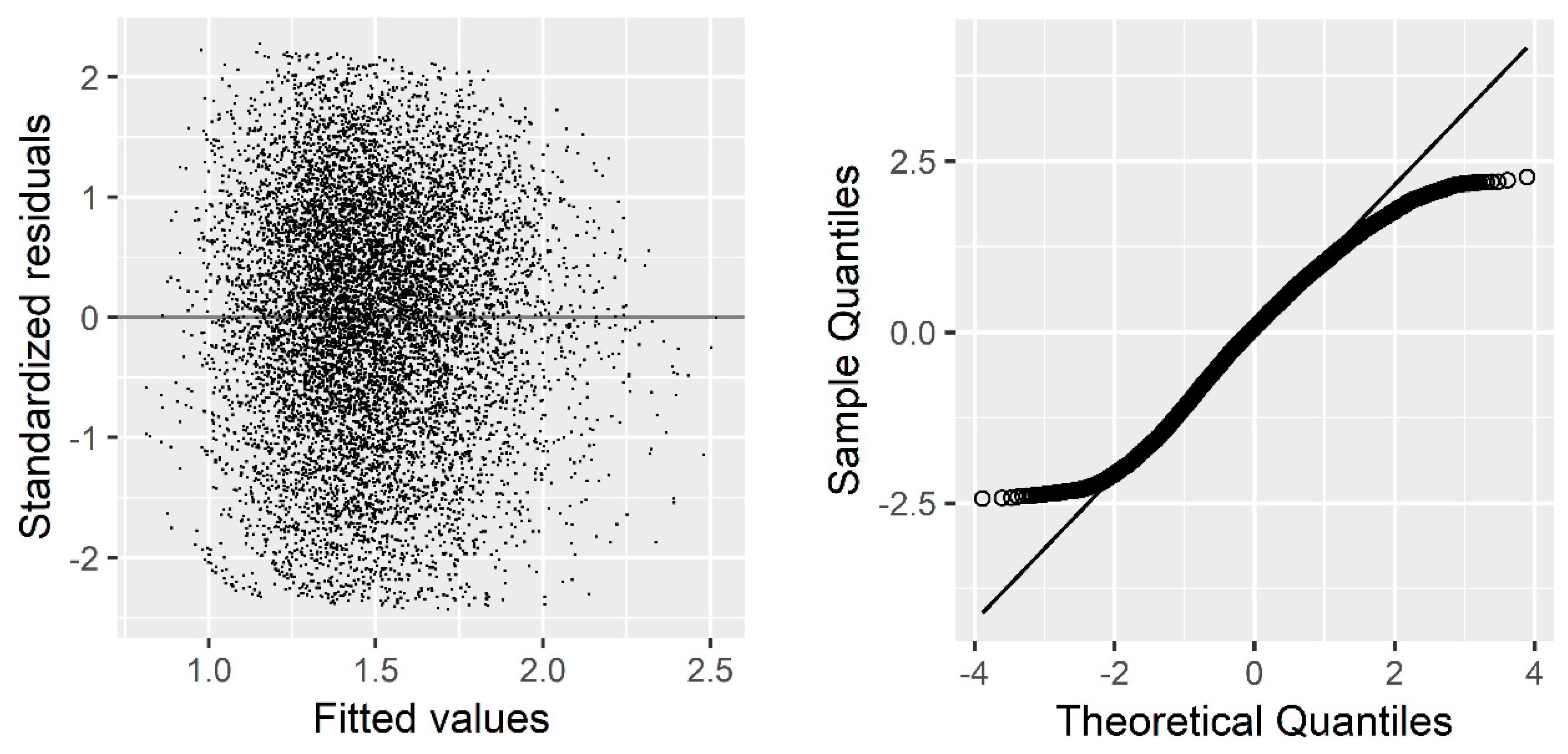
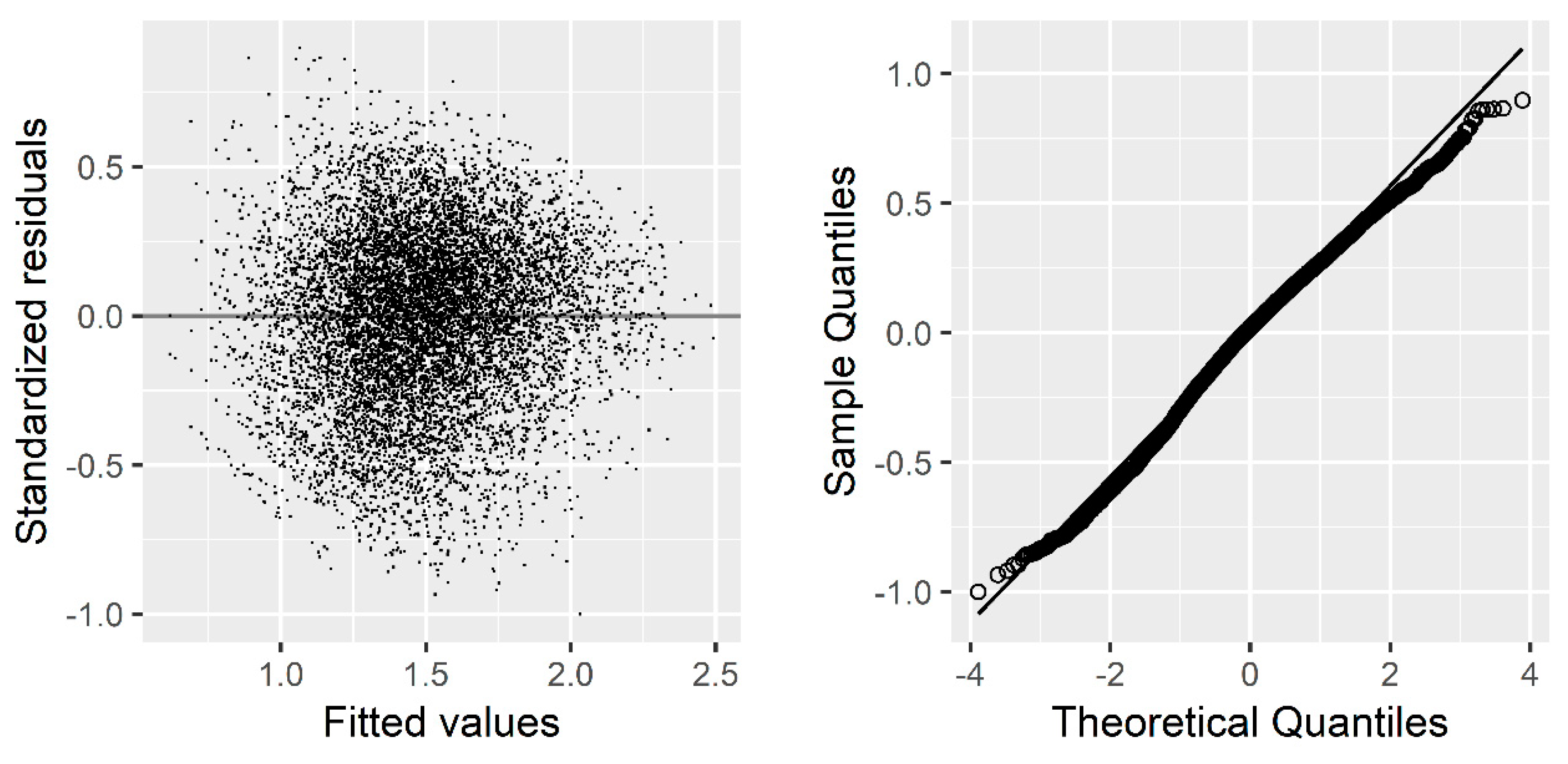
Although introducing random effects could correct or reduce autocorrelation and heteroscedasticity [65,68,87,88], our mixed-effects model still exhibited autocorrelation and heteroscedasticity. We therefore further introduced three variance functions and three correlation structures to refine our model. Finally, based on the lack-of-fit statistics, the exponent function and AR(1) were determined as the optimum option for correcting the heteroscedasticity and autocorrelation of the residuals. Similar results were also reported by Calama and Montero [47] and Fabian et al. [56]. Additionally, the model prediction and evaluation using validation data further supported the conclusion that the mixed-effects approach had significantly improved the model’s predictive performance, either in PA or SS in comparison to the basic model without random effects. For instance, the Bias decreased from 0.2239 to 0.1716, the RMSE decreased from 0.2776 to 0.2167 and the R² increased from 0.3663 to 0.6140.

Although the model performance was improved after we used the mixed-effects method to develop the individual-tree basal area increment model for oaks, there are some limitations of our final mixed-effects model. Firstly, we only considered the autocorrelation structure to correct autocorrelation. However, Zhao et al [65] reported that modelling the autocorrelation structure alone could not completely match the possible common effects and suggested introducing random period effect to describe autocorrelation, if data is sufficient. Pokharel and Dech [59] directly introduced random period effects to develop their diameter growth model. In the present study, unfortunately only three period observations were available for the same trees and hence it makes no sense to employ period as a random effect.

Secondly, climatic change has been widely reported to influence forest growth, productivity, tree species composition and distribution [89,90,91]. For instance, Battles et al. [92] assessed the impact of climate change on the productivity and health of the mixed-conifer forest in California and found that the productivity of stem volume increment was reduced by 19% in the most extreme climate change. Unfortunately, we did not include climatic variables due to lack of data. It is imperative to integrate climatic variables into forest growth models when data is available.

There are many individual-tree forest simulators throughout the world, for instance, the FVS, TASS, PROGNAUS in the US, the SILVA, and BWINPro in Germany and CAPSIS in France [93,94,95]. For a comprehensive prediction of forest dynamics, this individual-tree simulation system not only included individual-tree basal area or diameter increment models, but also integrated an individual-tree mortality and recruitment model. Therefore, the development of an individual-tree mortality and recruitment model of oak species is strongly recommended in the future.

5. Conclusion

In this study, we produced a linear mixed-effects individual-tree basal area increment model for oaks (Quercus spp.) that considers forest structural diversity. Our final model showed that it is necessary to consider forest structural diversity in model development. Additionally, compared with the basic model built by LASSO regression, the performance of the mixed-effects model was greatly improved. The model is a useful tool to predict the basal area growth of individual trees and propose relevant forest management strategies in uneven-aged mixed-species forests.

References

1. Nixon, K.C. Infrageneric classification of Quercus (Fagaceae) and typification of sectional names. Ann. Sci. For. 1993, 36, 25–34. [Google Scholar] [CrossRef]
2. Perea, R.; López-Sánchez, A.; Dirzo, R. Differential tree recruitment in California oak savannas: Are evergreen oaks replacing deciduous oaks? For. Ecol. Manage. 2017, 399, 1–8. [Google Scholar] [CrossRef] [Green Version]
3. Campos, P.; Huntsinger, L.; Oviedo, J.L.; Starrs, P.F.; Díaz, M.; Standiford, R.B.; Montero, G. Mediterranean Oak Woodland Working Landscapes: Dehesas of Spain and Ranchlands of California; Springer: Berlin, Germany, 2013; Volume 16. [Google Scholar]
4. Waldrop, M.P.; Firestone, M.K. Microbial Community Utilization of Recalcitrant and Simple Carbon Compounds: Impact of Oak-Woodland Plant Communities. Oecologia 2004, 138, 275–284. [Google Scholar] [CrossRef]
5. Ye, R.; Zhou, R.; Feng, J.; Chen, X. Studies on Soil Fertility and Function of Water Conservation of Oriental Oak Plantation in Northern Fujian. J. Fujian Coll. For. 1995, 15, 353–356. [Google Scholar] [CrossRef]
6. Harris, J.R.; Day, S.D. Planting depth at onset of container production and subsequent root ball remediation at transplanting affects pin oak and littleleaf linden. Hortscience 2010, 45, 1793–1797. [Google Scholar] [CrossRef]
7. Parent, C.; Crèvecoeur, M.; Capelli, N.; Dat, J.F. Contrasting growth and adaptive responses of two oak species to flooding stress: Role of non-symbiotic haemoglobin. Plant Cell Env. 2011, 34, 1113–1126. [Google Scholar] [CrossRef]
8. Wood, K.U.M. Ecological and Economic Impacts of Wildfires on an Appalachian Oak Forest in Southern West Virginia; West Virginia University: Morgantown, WV, USA, 2010. [Google Scholar]
9. Caprio, E.; Ellena, I.; Rolando, A. Native oak retention as a key factor for the conservation of winter bird diversity in managed deciduous forests in northern Italy. Landsc. Ecol. 2009, 24, 65. [Google Scholar] [CrossRef]
10. Chalupa, V. Somatic embryogenesis in oak (Quercus spp.). Vitro Cell. Dev. Biol. Plant 2000, 36, 349–357. [Google Scholar] [CrossRef]
11. Zadworny, M.; Jagodziński, A.M.; Łakomy, P.; Ufnalski, K.; Oleksyn, J. The silent shareholder in deterioration of oak growth: Common planting practices affect the long-term response of oaks to periodic drought. For. Ecol. Manag. 2014, 318, 133–141. [Google Scholar] [CrossRef]
12. Li, W.Y.; Wang, B.; Li, G.C. Ecological Benefits and Economic Values of Oaks Species and Countermeasures for Their Resource Protection. For. Sci. Techol. 2001, 8, 13–15. [Google Scholar] [CrossRef]
13. Jia, G.; Liu, Z.; Chen, L.; Yu, X. Distinguish water utilization strategies of trees growing on earth-rocky mountainous area with transpiration and water isotopes. Ecol. Evol. 2017, 7, 10640–10651. [Google Scholar] [CrossRef]
14. State Forestry Administration. Report of Forest Resources in China (2009–2013); China Forestry Press: Beijing, China, 2014.
15. Hou, Y.S.; Chen, X.L.; Sun, G.J. Oaks Management; China Forestry Press: Beijing, China, 2017. [Google Scholar]
16. Pang, Y.; Li, Z.; Huang, G.; Sun, G.; Cheng, Z.; Zhang, Z.; Zhang, G. China Forest Aboveground Biomass Estimation by Fusion of Inventory and Remote Sensing Data: 1st results from Heilongjiang Province and Yunnan Province. In Proceedings of the American Geophysical Union Fall Meeting, Washington, DC, USA, 9–13 December 2013. [Google Scholar]
17. Leites, L.P.; Robinson, A.L.; Crookston, N. Accuracy and equivalence testing of crown ratio models and assessment of their impact on diameter growth and basal area increment predictions of two variants of the Forest Vegetation Simulator. Can. J. For. Res. 2009, 39, 655–665. [Google Scholar] [CrossRef]
18. Weiskittel, A.R.; Hann, D.W.; Kershaw, J.A., Jr.; Vanclay, J.K. Forest Growth and Yield Modeling; John Wiley & Sons Incorporated: Hoboken, NJ, USA, 2011. [Google Scholar]
19. Pretzsch, H. Forest Dynamics, Growth and Yield; Springer: Berlin/Heidelberg, Germany, 2009. [Google Scholar]
20. Zhang, X. A linkage among whole-stand model, individual-tree model and diameter-distribution model. J. For. Sci. 2010, 56, 600–608. [Google Scholar] [CrossRef] [Green Version]
21. Burkhart, H.E.; Tomé, M. Modeling Forest Trees and Stands; Springer Science & Business Media: Berlin, Germany, 2012. [Google Scholar]
22. Lu, Y.C.; Luan, S.Q.; Zhang, S.G.; Heyde, B.V.D.; Lei, X.D.; Bao, Y. From normal forest to close-to-nature forest: Multi-functional forestry and its practice at national, regional and forest management unit levels in Germany. World For. Res. 2010, 23, 1–11. [Google Scholar] [CrossRef]
23. Porté, A.; Bartelink, H. Modelling mixed forest growth: A review of models for forest management. Ecol. Model. 2002, 150, 141–188. [Google Scholar] [CrossRef]
24. Peng, C. Growth and yield models for uneven-aged stands: Past, present and future. For. Ecol. Manag. 2000, 132, 259–279. [Google Scholar] [CrossRef]
25. Lhotka, J.M.; Loewenstein, E.F. An individual-tree diameter growth model for managed uneven-aged oak-shortleaf pine stands in the Ozark Highlands of Missouri, USA. For. Ecol. Manag. 2011, 261, 770–778. [Google Scholar] [CrossRef]
26. Wykoff, W.R. A basal area increment model for individual conifers in the northern Rocky Mountains. For. Sci. 1990, 36, 1077–1104. [Google Scholar] [CrossRef]
27. Weiskittel, A.R.; Garber, S.M.; Johnson, G.P.; Maguire, D.A.; Monserud, R.A. Annualized diameter and height growth equations for Pacific Northwest plantation-grown Douglas-fir, western hemlock, and red alder. For. Ecol. Manag. 2007, 250, 266–278. [Google Scholar] [CrossRef]
28. Kiernan, D.H.; Bevilacqua, E.; Nyland, R.D. Individual-tree diameter growth model for sugar maple trees in uneven-aged northern hardwood stands under selection system. For. Ecol. Manag. 2008, 256, 1579–1586. [Google Scholar] [CrossRef]
29. Sánchez-González, M.; Río, M.D.; Cañellas, I.; Montero, G. Distance independent tree diameter growth model for cork oak stands. For. Ecol. Manag. 2006, 225, 262–270. [Google Scholar] [CrossRef]
30. Huang, X.F.; Kang, X.G.; Sun, L.; Feng, Q.X.; Yao, J.C. Establishment of Individual Basal Area Growth of Korean Pine. J. Northwest For. Univ. 2011, 26, 143–146. [Google Scholar] [CrossRef]
31. Wang, J.J.; Zeng, W.S.; Meng, J.H. Individual-tree basal area growth model for Cunninghamia lanceolate with consideration of thinning and tree mortality in the prediction interval. J. Northwest For. Univ. 2017, 32, 181–185. [Google Scholar] [CrossRef]
32. Yan, M.Z.; Liu, Z.G. Study on growth of section area of breast height of Tilia amurensis individual tree of secondary forest in Mao’ershan mountain region. For. Eng. 2009, 25, 1–4. [Google Scholar] [CrossRef]
33. Pretzsch, H. Analysis and modeling of spatial stand structures. Methodological considerations based on mixed beech-larch stands in Lower Saxony. For. Ecol. Manag. 1997, 97, 237–253. [Google Scholar] [CrossRef]
34. Liang, J.; Buongiorno, J.; Monserud, R.A.; Kruger, E.L.; Zhou, M. Effects of diversity of tree species and size on forest basal area growth, recruitment, and mortality. For. Ecol. Manag. 2007, 243, 116–127. [Google Scholar] [CrossRef]
35. Lei, X.; Wang, W.; Peng, C. Relationships between stand growth and structural diversity in spruce-dominated forests in New Brunswick, Canada. Can. J. For. Res. 2009, 39, 1835–1847. [Google Scholar] [CrossRef]
36. Monleon, V.J. A hierarchical linear model for tree height prediction. In Proceedings of the 2003 Joint Statistical Meetings-Section on Statistics & the Environment, Alexandria, VA, USA, 3–7 August 2013; pp. 2865–2869. [Google Scholar]
37. Moses, L.E.; Gale, L.C.; Altmann, J. Methods for analysis of unbalanced, longitudinal, growth data. Am. J. Primatol. 2010, 28, 49–59. [Google Scholar] [CrossRef]
38. Biging, G.S. Improved estimates of site index curves using a varying-parameter model. For. Sci. 1985, 31, 248–259. [Google Scholar]
39. Kowalchuk, R.K.; Keselman, H.J. Mixed-model pairwise multiple comparisons of repeated measures means. Psychol. Method. 2001, 6, 282–296. [Google Scholar] [CrossRef]
40. Hayes, A.F.; Cai, L. Using heteroskedasticity-consistent standard error estimators in OLS regression: An introduction and software implementation. Behav. Res. Method. 2007, 39, 709–722. [Google Scholar] [CrossRef] [Green Version]
41. Fitzmaurice, G.M.; Laird, N.M.; Ware, J.H. Applied Longitudinal Analysis; Wiley: Hoboken, NJ, USA, 2011. [Google Scholar]
42. Gutzwiller, K.J.; Riffell, S.K. Using Statistical Models to Study Temporal Dynamics of Animal—Landscape Relations; Springer: Boston, MA, USA, 2007. [Google Scholar]
43. Hanke, J.E.; Wichern, D.W. Business Forecasting; Pearson: New York, NY, USA, 2008. [Google Scholar]
44. Goldstein, H. Multilevel mixed linear model analysis using iterative generalized least squares. Biometrika 1986, 73, 43–56. [Google Scholar] [CrossRef]
45. Morris, J.S.; Arroyo, C.; Coull, B.A.; Ryan, L.M.; Gortmaker, H.S.L. Using Wavelet-Based Functional Mixed Models to Characterize Population Heterogeneity in Accelerometer Profiles: A Case Study. J. Am. Stat. Assoc. 2006, 101, 1352–1364. [Google Scholar] [CrossRef]
46. Vonesh, E.F.; Chinchilli, V.M. Linear and nonlinear models for the analysis of repeated measurements. J. Biopharm. Stat. 1996, 18, 595–610. [Google Scholar] [CrossRef]
47. Calama, R.; Montero, G. Multilevel Linear Mixed Model for Tree Diameter Increment in Stone Pine (Pinus pinea): A Calibrating Approach. Silva. Fennica 2005, 39, 37–54. [Google Scholar] [CrossRef]
48. Zobel, J.M.; Ek, A.R.; Burk, T.E. Comparison of Forest Inventory and Analysis surveys, basal area models, and fitting methods for the aspen forest type in Minnesota. For. Ecol. Manag. 2011, 262, 188–194. [Google Scholar] [CrossRef]
49. Sharma, M.; Parton, J. Height–diameter equations for boreal tree species in Ontario using a mixed-effects modeling approach. For. Ecol. Manag. 2007, 249, 187–198. [Google Scholar] [CrossRef]
50. Crecente-Campo, F.; Tomé, M.; Soares, P.; Diéguez-Aranda, U. A generalized nonlinear mixed-effects height–diameter model for Eucalyptus globulus L. in northwestern Spain. For. Ecol. Manag. 2010, 259, 943–952. [Google Scholar] [CrossRef]
51. Fu, L.; Sharma, R.P.; Hao, K.; Tang, S. A generalized interregional nonlinear mixed-effects crown width model for Prince Rupprecht larch in northern China. For. Ecol. Manag. 2017, 389, 364–373. [Google Scholar] [CrossRef]
52. Hao, X.; Yujun, S.; Xinjie, W.; Jin, W.; Yao, F. Linear mixed-effects models to describe individual tree crown width for China-fir in Fujian Province, southeast China. PLoS ONE 2015, 10, e0122257. [Google Scholar] [CrossRef]
53. Vanderschaaf, C.; Burkhart, H. Comparison of Methods to Estimate Reineke’s Maximum Size-Density Relationship Species Boundary Line Slope. For. Sci. 2007, 53, 435–442. [Google Scholar]
54. Zhang, L.; Bi, H.; Gove, J.H.; Heath, L.S. A comparison of alternative methods for estimating the self-thinning boundary line. Can. J. For. Res. 2005, 35, 1507–1514. [Google Scholar] [CrossRef]
55. Weiskittel, A.; Gould, P.; Temesgen, H. Sources of variation in the self-thinning boundary line for three species with varying levels of shade tolerance. For. Sci. 2009, 55, 83–93. [Google Scholar] [CrossRef]
56. Uzoh, F.C.C.; Oliver, W.W. Individual tree diameter increment model for managed even-aged stands of ponderosa pine throughout the western United States using a multilevel linear mixed effects model. For. Ecol. Manag. 2008, 256, 438–445. [Google Scholar] [CrossRef]
57. Hart, D.R.; Chute, A.S. Estimating von Bertalanffy growth parameters from growth increment data using a linear mixed-effects model, with an application to the sea scallop Placopecten magellanicus. ICES J. Mar. Sci. 2009, 66, 2165–2175. [Google Scholar] [CrossRef]
58. Condés, S.; Sterba, H. Comparing an individual tree growth model for Pinus halepensis Mill. in the Spanish region of Murcia with yield tables gained from the same area. Eur. J. For. Res. 2008, 127, 253–261. [Google Scholar] [CrossRef]
59. Pokharel, B.; Dech, J.P. Mixed-effects basal area increment models for tree species in the boreal forest of Ontario, Canada using an ecological land classification approach to incorporate site effects. Forestry 2012, 85, 255–270. [Google Scholar] [CrossRef] [Green Version]
60. Stage, A.R. An Expression for the Effect of Aspect, Slope, and Habitat Type on Tree Growth. For. Sci. 1976, 22, 457–460. [Google Scholar] [CrossRef]
61. Jinghui, M.; Shiming, L.; Wei, W.; Qingwang, L.; Shiqin, X.; Wu, M. Estimation of forest structural diversity using the spectral and textural information derived from spot-5 satellite images. Remote Sens. 2016, 8, 125–149. [Google Scholar]
62. Hökkä, H.; Alenius, V.; Penttilä, T. Individual-tree basal area growth models for Scots pine, pubescent birch and Norway spruce on drained peatlands in Finland. Silva. Fennica 1997, 31, 161–178. [Google Scholar] [CrossRef]
63. Patricia, A.; Jari, H.; Isabel, C.; Miren, D.R. Individual-tree diameter growth model for rebollo oak (Quercus pyrenaica Willd.) coppices. For. Ecol. Manag. 2008, 255, 1011–1022. [Google Scholar] [CrossRef]
64. Paulo, C.; Sebastian, P.; Francisco, J.E.; Wendell, P.C.; Salvador, A.G. Individual-tree diameter growth models for mixed nothofagus second growth forests in southern Chile. Forests 2017, 8, 506. [Google Scholar] [CrossRef]
65. Zhao, L.F.; Li, C.M.; Tang, S.Z. Individual-tree diameter growth model for fir plantations based on multi-level linear mixed effects models across southeast China. J. For. Res. 2013, 18, 305–315. [Google Scholar] [CrossRef]
66. Hall, D.B.; Bailey, R.L. Modeling and prediction of forest growth variables based on multilevel nonlinear mixed models. For. Sci. 2001, 47, 311–321. [Google Scholar] [CrossRef]
67. Yang, Y.; Huang, S.; Meng, S.X.; Trincado, G.; Vanderschaaf, C.L. A multilevel individual tree basal area increment model for aspen in boreal mixedwood stands. Can. J. For. Res. 2009, 39, 2203–2214. [Google Scholar] [CrossRef]
68. Gregoire, T.G. Generalized error structure for forestry yield models. For. Sci. 1987, 33, 423–444. [Google Scholar]
69. Davidian, M.; Giltinan, D.M. Nonlinear models for repeated measurement data: An overview and update. Technometrics 2015, 38, 186–187. [Google Scholar] [CrossRef]
70. Pinheiro, J.C.; Bates, D.M. Mixed-effects models in S and S-Plus. J. Am. Stat. Assoc. 2000, 96, 1135–1136. [Google Scholar]
71. Gilbert, G.E. Linear Mixed Models: A Practical Guide Using Statistical Software. J. Am. Stat. Assoc. 2008, 103, 427–428. [Google Scholar] [CrossRef]
72. Liyong, F.; Huiru, Z.; Jun, L.; Hao, Z.; Minghua, L.; Guangxing, W. Multilevel Nonlinear Mixed-Effect Crown Ratio Models for Individual Trees of Mongolian Oak (Quercus mongolica) in Northeast China. PLoS ONE 2015, 10, e0133294. [Google Scholar] [CrossRef]
73. Cao, Q.V.; Li, S.; Mcdill, M.E. Developing a system of annual tree growth equations for the loblolly pine—shortleaf pine type in Louisiana. Can. J. For. Res. 2002, 32, 2051–2059. [Google Scholar] [CrossRef]
74. Lei, X.D.; Li, Y.C.; Xiang, E. Individual basal area growth model using multi-level linear mixed model with repeated measures. Sci. Silvae Sin. 2009, 45, 74–80. [Google Scholar] [CrossRef]
75. Timilsina, N.; Staudhammer, C.L. Individual Tree-Based Diameter Growth Model of Slash Pine in Florida Using Nonlinear Mixed Modeling. For. Sci. 2013, 59, 27–37. [Google Scholar] [CrossRef]
76. Cannell, M.G.R.; Rothery, P.; Ford, E.D. Competition Within Stands of Picea sitchensis and Pinus contorta. Ann. Bot. 1984, 53, 349–362. [Google Scholar] [CrossRef] [Green Version]
77. Ma, X.; Heal, K.V.; Liu, A.; Jarvis, P.G. Nutrient cycling and distribution in different-aged plantations of Chinese fir in southern China. For. Ecol. Manag. 2007, 243, 61–74. [Google Scholar] [CrossRef]
78. Yu, L.; Jia, W.W.; Liu, G.C.; Zhang, H.T. Single Tree Growth Model of Larix Gmelinii Plantation in zhangguangcailing area. For. Sci. Technol. Inf. 2018, 50, 1–4. [Google Scholar]
79. Weiner, J. Asymmetric competition in plant populations. Trends Ecol. Evol. 1990, 5, 360–364. [Google Scholar] [CrossRef]
80. Soares, P.; Tomé, M. GLOBTREE: An individual tree growth model for Eucalyptus globulus in Portugal. In Modelling Forest Systems; CABI Publishing: Wallingford, UK, 2003; pp. 97–110. [Google Scholar]
81. Casper, B.B.; Jackson, R.B. Plant competition underground. Annu. Rev. Ecol. Syst. 1997, 28, 545–570. [Google Scholar] [CrossRef]
82. Brown, H.G.; Loewenstein, H. Predicting site productivity of mixed conifer stands in northern Idaho from Soil and Topographic Variables1. Soil Sci. Soc. Am. J. 1978, 42, 967–971. [Google Scholar] [CrossRef]
83. Uzoh; Fabian, C.C. A height increment equation for young ponderosa pine plantations using precipitation and soil factors. For. Ecol. Manag. 2001, 142, 193–203. [Google Scholar] [CrossRef]
84. Wang, A.; Wang, X.; Tognetti, R.; Lei, J.P.; Pan, H.L.; Liu, X.L.; Jiang, Y.; Wang, X.Y.; He, P.; Yu, F.H. Elevation alters carbon and nutrient concentrations and stoichiometry in Quercus aquifolioides in southwestern China. Sci. Total Env. 2018, 622, 1463–1475. [Google Scholar] [CrossRef]
85. Cordonnier, T.; Kunstler, G. The Gini index brings asymmetric competition to light. Perspect. Plant Ecol. 2015, 17, 107–115. [Google Scholar] [CrossRef]
86. Bourdier, T.; Cordonnier, T.; Kunstler, G.; Piedallu, C.; Lagarrigues, G.; Courbaud, B. Tree size inequality reduces forest productivity: An analysis combining inventory data for ten European species and a light competition model. PLoS ONE 2016, 11, e0151852. [Google Scholar] [CrossRef] [PubMed]
87. Wang, Y.; Lemay, V.M.; Baker, T.G. Modelling and prediction of dominant height and site index of Eucalyptus globulus plantations using a nonlinear mixed-effects model approach. Can. J. For. Res. 2007, 37, 1390–1403. [Google Scholar] [CrossRef]
88. Meng, S.X.; Huang, S.; Vanderschaaf, C.L.; Yang, Y.; Trincado, G. Accounting for serial correlation and its impact on forecasting ability of a fixed- and mixed-effects basal area model: A case study. Eur. J. For. Res. 2012, 131, 541–552. [Google Scholar] [CrossRef]
89. Boden, S.; Pyttel, P.; Eastaugh, C.S. Impacts of climate change on the establishment, distribution, growth and mortality of Swiss stone pine (Pinus cembra L.). Ifor. Biogeosciences For. 2010, 3, 82–85. [Google Scholar] [CrossRef]
90. Eastaugh, C.S.; Pötzelsberger, E.; Hasenauer, H. Assessing the impacts of climate change and nitrogen deposition on Norway spruce (Picea abies L. Karst) growth in Austria with BIOME-BGC. Tree Physiol. 2011, 31, 262–274. [Google Scholar] [CrossRef] [PubMed]
91. Cailleret, M.; Heurich, M.; Bugmann, H. Reduction in browsing intensity may not compensate climate change effects on tree species composition in the Bavarian Forest National Park. For. Ecol. Manag. 2014, 328, 179–192. [Google Scholar] [CrossRef]
92. Battles, J.J.; Robards, T.; Das, A.; Waring, K.; Gilless, J.K.; Biging, G.; Schurr, F. Climate change impacts on forest growth and tree mortality: A data-driven modeling study in the mixed-conifer forest of the Sierra Nevada, California. Clim. Chang. 2008, 87, 193–213. [Google Scholar] [CrossRef]
93. Albrecht, A.; Hein, S.; Kohnle, U.; Biber, P. Evaluation of the single-tree based growth simulator SILVA 2.2 using long-term experimental plots with contrasting thinning regimes. Allg. Forst Jagdztg. 2009, 180, 55–64. [Google Scholar] [CrossRef]
94. Nagel, J.; Schmidt, M. The Silvicultural Decision Support. System BWINPro; Springer: Berlin/Heidelberg, Germany, 2006. [Google Scholar]
95. Dufour-Kowalski, S.; Courbaud, B. Capsis: An open software framework and community for forest growth modelling. Ann. For. Sci. 2012, 69, 221–233. [Google Scholar] [CrossRef]
Figure 1. Distribution of the inventory sample plots for oaks in the studied area.
Forests 10 00474 g001
Figure 2. Residual plot and quantile–quantile (QQ) plot (QQ plot depicts the observed values against its standardised normal distribution) of the basic model.
Forests 10 00474 g002
Figure 3. Residual plot and QQ plot of our final mixed-effects model.
Forests 10 00474 g003
Figure 4. Predicted DBH increments derived from the basic model (Equation (24)) and mixed-effects model (Equation (26)) over DBH with all other predictors set to their mean for oaks in Hunan Province, south-central China.
Forests 10 00474 g004